On Stability and Sojourn Time of Peer-to-Peer Queuing Systems

Classical queueing theory have been a useful tool on modeling systems where jobs arrive randomly at static service stations of given service capacities. It provides analysis of the system’s properties, such as stability and sojourn time. Queueing theory has wide application in many scenarios of operations research. In particular, its application in studying computer networks and operating systems led to a generalization of queueing theory to model a network of queues and many different service policies [1, 2].

Recently, the modeling of peer-to-peer (P2P) systems is pointing to a new kind of queueing system. In this new model, jobs still arrive randomly, but the service stations also arrive randomly [3]. This new model, if well studied, would be helpful on the quality of service study of different kinds of peer-to-peer systems, such as online storage or video-on-demand systems[4].

However, current study on the performance of this new model has been limited on the system stability condition only, and under exponential workload assumptions. In this paper we extend this result on two aspects. We first relax the exponential workload assumption, and prove that a P2P queuing system with general workload distribution would still have the same stability condition as the system with exponential workload. Then we turn ourselves go beyond stability and study the sojourn time of the p2p queuing systems under the exponential workload assumption. Such sojourn time is challenging to derive. We provide an upper bound and a lower bound for it, and show the bound is tight by numerical analysis.

The rest of the paper is organized as followed: We first brief introduce the related work on peer-to-peer system modeling and queueing model with dynamic service rate in section II, and list the basic notations and assumptions in section III. Then in section IV we study the system stability without exponential assumption. Upper and lower bounds of average queue length is derived in section V. Section VI gives some numerical results. The work is concluded in section VII.

The modeling of P2P systems have received a lot of attention from researchers in the past years. One of the first dynamic P2P models was introduced by Qiu and Srikant [5] to model BitTorrent, a P2P file sharing system. The model is simple, but very inspiring. Although they did not mention queueing theory, they implicitly modeled randomly arriving service stations (which are peers themselves) providing an effective service (file sharing) rate. Subsequently, Fan, Chiu and Lui [6] modeled and studied the tradeoff between different service rate allocations in a dynamic P2P system similar to the Qiu-Srikant model.

Clevenot, Nain and Ross [7] generalized the Qiu-Srikant model fluid model to describe more realistic cases. The authors in [8] and [9] also used randomly arriving peers with certain service rate to model P2P streaming systems.

On the other hand, the queuing model with dynamic service have been preliminarily studied in other areas, such as in modeling transportation system [10]. There are also research on performance of a queuing system with varying service rate. However, these works lies in two extreme cases. Some of them focus on special case that there is only two state of service rate: “normal” and “disrupted”[10, 11]. While rests study models which are too general that they can only give numerical results [12, 13, 14]. Both of them are not suitable to study P2P systems, where service rate may varies proportionally with the number of available servers in the system. Our previous work[3] models this kind of systems, and gives a preliminary study.

This paper is based on the framework of P2P queuing model proposed in our previous work[3]. The notations used in the framework are listed in Table I.

In classical queuing theory, Kendall’s notation [1], i.e., $\mbox{A}/\mbox{B}/\mbox{s}$, is widely used to represent queuing model for static service systems where servers are static.

To represent new queuing models for P2P service systems in which both job and server dynamically arrive and depart, we use the notation

$$\mbox{A}/\mbox{B}/(\mbox{C}/\mbox{E}).$$

(1)

This notation extends Kendall’s notation, by using two additional terms (C and E) to represent the server dynamics in P2P queuing models.

To represent systems with different job and server dynamics, some notations we use for arrival processes (A or C) and distributions (B or E) are 1) $M$ for a memoryless process (e.g. Poisson process), or an exponential distribution. 2) $D$ for a deterministic process, or a deterministic distribution. 3) $G$ for a process with general independent arrivals, or arbitrary distribution.

In this paper we mainly discuss about $M/M/(M/M)$ and $M/G/(M/M)$ systems, with two basic assumptions:

1. 1.

   Servers are homogeneous and each has a unit service capacity.

2. 2.

   Job arrival are independent to the server process.

Our previous work[3] has discussed the stability of an $M/M/(M/M)$ queuing system, in the semantic in the positive recurrence of the job process, resulting in Theorem.2.

Note that if the Markov process $\left\{n_{c}(t),n_{s}(t)\right\}_{t}$ is stable, then not only it has a stationary distribution, but also the states $(n_{c}=0,n_{s}=j),(0\leq j)$, will be visited within finite amount of time. Practically, this means that all arriving jobs will be served and cleared by the P2P service system in finite time.

However in practice, job workload distribution (file length distribution in a P2P storage system or video chunk size distribution in a P2P streaming system), are not exponential [15]. This observation motivates us to study the stability of $M/G/(M/M)$ queuing systems.

In order to do this, we consider a discrete time version of $M/G/(M/M)$ system with the number of servers bounded by $n_{s}\leq M_{s}$. The stability condition for this system should be stronger than that of the $M/G/(M/M)$ system. Consequently, sufficient conditions for the modified system to be stable also suffice to warranty the stability of $M/G/(M/M)$ systems.

The job-server process of such a discrete time system is a 2-D discrete time Markov chain $(X,n_{s})$ with transition probability given in Table II.

Note that:

1. 1.

   It is a discrete time system with time slot interval $\Delta t$. We choose $\Delta t$ to be small enough so that only one event (job arrival, server arrival, server departure) happens in one slot, since the probability that two events happen in a single time slot is $O(\Delta t^{2})$. When $\Delta t\rightarrow 0$, the discrete time system approaches a continuous time system.

2. 2.

   We assume the distribution of job workload $X_{n}$ is discrete, as

   $$P(X_{n}=L_{i})=p_{i},\frac{L_{i}}{\Delta t}\in\mathbb{N}.$$

3. 3.

   As a conservative approximation, when number of servers changes in a time slot, we use the minimal number of servers to calculate the service amount in the slot.

4. 4.

   The transition probability in the table is only for the non-boundary part of the process $(X>n_{s}\Delta t,0<n_{s}<M_{s})$. The boundary part should be discussed independently.

In order to find the stability condition of the system, we use the Foster-Lyapunov criteria. That is, we try to find a Foster-Lyapunov function and apply the following theorem.

The stability condition for M/G/(M/M) systems is given in the following theorem.

To prove the stability of the system, we construct a function $V(X,n_{s})$ as

$$V=k\mu_{c}X+(n_{s}-\rho_{s})^{2}+mn_{s}.$$

For this function $V$, it can be seen that any $k>0$ would make $\{(X,n_{s})|V(X,n_{s})<\epsilon\}$ a finite set for $\forall\epsilon>0$.

We further observe that

	$\displaystyle\Delta V$	$\displaystyle=$	$\displaystyle k(\lambda_{c}-n_{s}\mu_{c})\Delta t+n_{s}\mu_{c}\mu_{s}\Delta t^{2}$
		$\displaystyle+$	$\displaystyle m(\lambda_{s}-n_{s}\mu_{s})\Delta t+(\lambda_{s}+n_{s}\mu_{s}-2\mu_{s}(n_{s}-\rho_{s})^{2})\Delta t.$

It can be shown that as long as $\rho_{c}/\rho_{s}<1$, there exists a tuple $(k>0,m\in\mathbb{R})$ so that $\Delta V<0$ for all $n_{s}\geq 0$. For example, let

	$\displaystyle k$	$\displaystyle=$	$\displaystyle\frac{\mu_{s}}{\mu_{c}}(2\rho_{s}-2\rho_{c}+2\frac{\rho_{s}}{\rho_{s}-\rho_{c}}+1),$		(4)
	$\displaystyle m$	$\displaystyle=$	$\displaystyle 2(\rho_{s}-\rho_{c})-2\frac{\rho_{s}}{\rho_{s}-\rho_{c}}.$		(5)

We have

$$\frac{\Delta V}{\Delta t}=-2\mu_{s}(n_{s}-\rho_{c})^{2}+\mu_{s}(\rho_{c}-\rho_{s}).$$

(6)

Since $\rho_{c}<\rho_{s}$, we have $\Delta V<0$ for all $(X\geq 0,n_{s}\geq 0)$.

However, this transition probability is only for the non-boundary part. Then when process is at boundary, $\frac{\Delta V}{\Delta t}$ would not equal to

	$\displaystyle W$	$\displaystyle\triangleq$	$\displaystyle k(\lambda_{c}-n_{s}\mu_{c})+n_{s}\mu_{c}\mu_{s}\Delta t$
		$\displaystyle+$	$\displaystyle m(\lambda_{s}-n_{s}\mu_{s})+\lambda_{s}+n_{s}\mu_{s}-2\mu_{s}(n_{s}-\rho_{s})^{2}$

So we need to reexamine that whether $\Delta V<0$ still holds on the boundary.

1. 1.

   $X<n_{s}\Delta t$ bound

   On this boundary, we have $\Delta X>\lambda_{c}\Delta t-n_{s}\mu_{c}\Delta t$, so $\Delta V>W\Delta t$. However, we still have that $\Delta X<\lambda_{c}\Delta t$, which would lead to

   $$\frac{\Delta V}{\Delta t}<W+n_{s}\mu_{c}.$$

   Notice here the set $\{n_{s}|\Delta V\geq 0,n_{s}\geq 0\}$ is finite. Since we have $X<n_{s}\Delta t$, $\{(X,n_{s})|\Delta V\geq 0,X\geq 0,n_{s}\geq 0\}$ is also finite.

2. 2.

   $n_{s}=0$ bound

   On this boundary, we still have $\Delta V=W\Delta t$. Thus we have $\Delta V<0$.

3. 3.

   $n_{s}=M_{s}$ bound

   On this boundary, we have

   $$\frac{\Delta V}{\Delta t}=W-\lambda_{s}(m+1+2(n_{s}-\rho_{s})).$$

   Thus if we choose an $M_{s}$ large enough, or $M_{s}>\rho_{s}-(m+1)/2$, we would still have $\Delta V<0$ on this boundary. If we use

   $$m=2(\rho_{s}-\rho_{c})-2\frac{\rho_{s}}{\rho_{s}-\rho_{c}}$$

   as mentioned, this condition would became

   $$M_{s}>\rho_{c}+\frac{\rho_{s}}{\rho_{s}-\rho_{c}}-\frac{1}{2}.$$

In the summary of non-boundary and boundary part, we have shown that function $V$ satisfies the condition that $\{(X,n_{s})|\Delta V(X,n_{s})\geq 0\}$ is a finite set. Applying Theorem 3, we show that process $\left\{X(t),n_{s}(t)\right\}_{t}$ is positive recurrent, and thus the $M/G/(M/M)$ system is stable.

This result indicates that the relax of exponential workload assumption have no effect on the stability condition of the system. Study on stability of more general systems (e.g. $G/G/(G/G)$) would be interesting.

Besides stability, another important metrics of a service system would be the average sojourn time of jobs came into the system, which affects user experience. A common way to study sojourn time would be looking at average queue length: with Little’s law, average queue length can be simply converted into average sojourn time. Since study on a system with general job workload is quite difficult, here we focus on $M/M/(M/M)$ system, where job workload is exponential.

An $M/M/(M/M)$ system can be modeled as a 2-D Markov chain $\left\{n_{c}(t),n_{s}(t)\right\}_{t}$. The transition rate is listed in Table III.

Our purpose is to get the average queue length, or $E[n_{c}]$. The basic method to get $E[n_{c}]$ is to study the balance equation of the process, and to solve equilibrium probability

$$\pi_{ij}=P(n_{s}=i,n_{c}=j).$$

However, since this 2-D Markov process is non time-reversible and have infinite state, it is unable to give the close form of equilibrium distribution. However, we are able to give the following bound.

Note that, the lower bound $\rho_{c}/(\rho_{s}-\rho_{c})$ is exactly the average queue length of an $M/M/s$ system, where the server amount equals to $\rho_{s}$, which is the average server amount in $M/M/(M/M)$. This result means that, with the same average service capacity, a system with server dynamic would always perform worse than a static system.

When system load $\rho_{c}$ varies, the upper bound remains proportional with the lower bound, with a coefficient $\mu_{c}/\mu_{s}+1$. This result implies that, the system with higher server dynamics (which means a larger $\mu_{s}$) would performs closer with a static system. This result answers the simulation result in [3].

To prove the former bounds, we need the following conjecture.

The intuition of this conjecture is easy to understand. If the $\{n_{c}\}$ and $\{n_{s}\}$ processes are fully decoupled, their correlation should be zero. In $M/M/(M/M)$ system, however, the departure rate of $n_{c}$ is proportional with $n_{s}$. So that when $n_{s}$ is large, $n_{c}$ tend to be smaller than when $n_{s}$ is smaller. That infers the negative correlation between $\{n_{c}\}$ and $\{n_{s}\}$. However, the rigorous proof is still missing by now. We will verify this conjecture by numerical results in the next section.

To prove the bounds of the average waiting time, we study the generating function $F(Z,W)$ of the process, defined as

$$F(Z,W)=\sum_{i=0}^{\infty}\sum_{j=0}^{\infty}\pi_{ij}Z^{i}W^{j}.$$

(9)

We further define

	$\displaystyle H_{0}(W)$	$\displaystyle=$	$\displaystyle\sum_{j=0}^{\infty}\pi_{0j}W^{j}$		(10)
	$\displaystyle G_{0}(Z)$	$\displaystyle=$	$\displaystyle\sum_{i=0}^{\infty}\pi_{i0}Z^{i}$		(11)

as the edge functions. By combining definitions with the balance equation, we know that $F(Z,W)$ satisfies the following differential equation:

			$\displaystyle(\mu_{s}+\mu_{c}\frac{Z}{W}-\mu_{s}Z-\mu_{c}Z)\frac{\partial F}{\partial Z}+\mu_{c}(1-\frac{1}{W})ZG_{0}^{\prime}(Z)$		(12)
		$\displaystyle=$	$\displaystyle(\lambda_{c}+\lambda_{s}-\lambda_{c}W-\lambda_{s}Z)F$

By definition, we have a series of relationships between moments of state variables and derivatives of generating function at the point $(Z=1,W=1)$, as follows.

	$\displaystyle F(1,1)$	$\displaystyle=$	$\displaystyle 1$		(13)
	$\displaystyle\frac{\partial F}{\partial Z}(1,1)$	$\displaystyle=$	$\displaystyle E[n_{s}]$		(14)
	$\displaystyle\frac{\partial F}{\partial W}(1,1)$	$\displaystyle=$	$\displaystyle E[n_{c}]$		(15)
	$\displaystyle\frac{\partial^{2}F}{\partial Z^{2}}(1,1)$	$\displaystyle=$	$\displaystyle E[n_{s}(n_{s}-1)]$		(16)
	$\displaystyle\frac{\partial^{2}F}{\partial Z\partial W}(1,1)$	$\displaystyle=$	$\displaystyle E[n_{s}n_{c}]$		(17)
	$\displaystyle G_{0}(1)$	$\displaystyle=$	$\displaystyle P(n_{c}=0)$		(18)
	$\displaystyle G_{0}^{\prime}(1)$	$\displaystyle=$	$\displaystyle E[n_{s}|n_{c}=0]P(n_{c}=0)$		(19)
	$\displaystyle G_{0}^{\prime\prime}(1)$	$\displaystyle=$	$\displaystyle E[n_{s}(n_{s}-1)|n_{c}=0]P(n_{c}=0)$		(20)

Thus by applying partial derivatives to (12) and let $Z=1,W=1$, we were able to get result on the moments of $n_{c}$ and $n_{s}$.

Applying $\frac{\partial}{\partial Z}$:

$$E[n_{s}]=\rho_{s}$$

(21)

Applying $\frac{\partial}{\partial W}$:

$$G_{0}^{\prime}(1)=E[n_{s}]-\rho_{c}$$

(22)

Applying $\frac{\partial^{2}}{\partial Z^{2}}$:

$$E[n_{s}(n_{s}-1)]=\rho_{s}E[n_{s}]$$

(23)

Applying $\frac{\partial^{2}}{\partial W^{2}}$:

$$\rho_{c}E[n_{c}]=E[n_{s}n_{c}]-E[n_{s}]+G_{0}^{\prime}(1)$$

(24)

Applying $\frac{\partial^{2}}{\partial Z\partial W}$:

			$\displaystyle\lambda_{c}E[n_{s}]+\lambda_{s}E[n_{c}]=\mu_{c}E[n_{s}(n_{s}-1)]+\mu_{s}E[n_{s}n_{c}]$		(25)
		$\displaystyle+$	$\displaystyle\mu_{c}E[n_{s}]-\mu_{c}(G_{0}^{\prime}(1)+G_{0}^{\prime\prime}(1))$

Combination based on (24) gives

$$E[n_{c}]=\frac{\rho_{c}}{\rho_{c}-\rho_{s}}-\frac{\text{Cor}[n_{c},n_{s}]}{\rho_{s}}.$$

(26)

Since $\text{Cor}[n_{c},n_{s}]<0$, we have

$$E[n_{c}]>\frac{\rho_{c}}{\rho_{c}-\rho_{s}}.$$

(27)

Combination based on (25) gives

$$E[n_{c}]=\frac{\frac{\mu_{c}}{\mu_{s}}+1}{\frac{\rho_{s}}{\rho_{c}}-1}+\frac{\mu_{c}}{\mu_{s}}\left(\rho_{s}-\frac{G_{0}^{\prime\prime}(1)}{\rho_{s}-\rho_{c}}\right).$$

(28)

Notice that

$$\frac{G_{0}^{\prime\prime}(1)}{\rho_{s}-\rho_{c}}=\frac{E[n_{s}(n_{s}-1)|n_{c}=0]}{E[n_{s}]|n_{c}=0}.$$

(29)

Since $n_{s}$ and $n_{c}$ have a negative correlation, there is

$$\frac{E[n_{s}(n_{s}-1)|n_{c}=0]}{E[n_{s}|n_{c}=0]}>\frac{E[n_{s}(n_{s}-1)]}{E[n_{s}]}=\rho_{s},$$

(30)

which gives

$$E[n_{c}]<(\frac{\mu_{c}}{\mu_{s}}+1)\frac{\rho_{c}}{\rho_{s}-\rho_{c}}.$$

(31)

We use matrix geometric analysis[17, 18] to get a numerical result of the equilibrium distribution and then average waiting time of the system. We compare the numerical result with the bounds we derived in the last section. The result lies in Fig.1. (System parameter is $\rho_{s}=10$, $\mu_{s}=1$, $\mu_{c}=10$, varying $\lambda_{c}$ so that $\rho_{c}$ changes.)

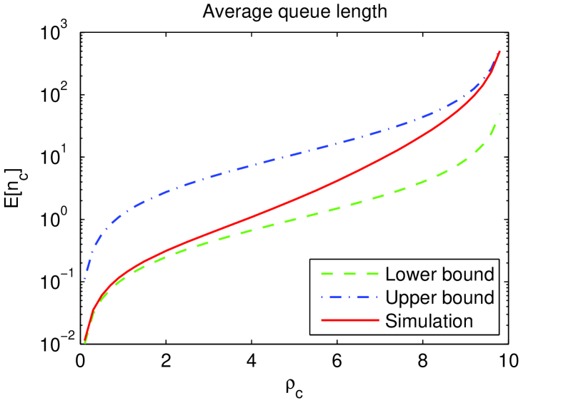
From the simulation result we see that when $\rho_{c}\approx 0$, or the system is in light load, the average queue length is close to the lower bound $1/(\frac{\rho_{s}}{\rho_{c}}-1)$. While when $\rho_{c}\approx\rho_{s}$, or the system load is heavy, the average queue length is close to the upper bound $(\frac{\mu_{c}}{\mu_{s}}+1)/(\frac{\rho_{s}}{\rho_{c}}-1)$.

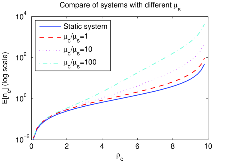
Fig.2. compares systems with different server dynamics. All the systems have the same average number of servers $\rho_{s}=10$, but have different $\mu_{c}/\mu_{s}$. Result shows that with light load, all the systems perform closely. But when the load is heavy, the average queue length is nearly proportional with $\mu_{c}/\mu_{s}+1$, thus system with higher server dynamics will perform much better under a heavy load.

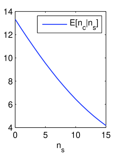
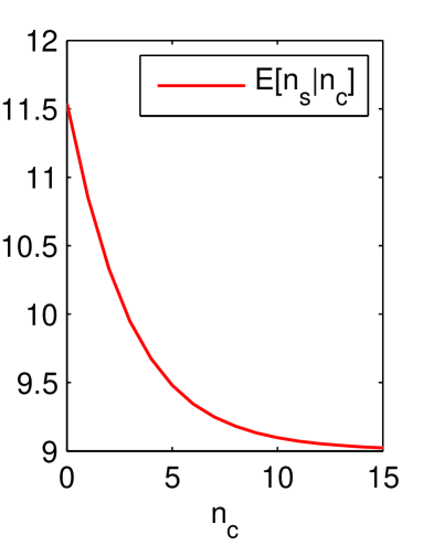
We also run simulation to verify the negative correlation between $n_{c}$ and $n_{s}$ claimed in Conj.7. Conditional expectations $E[n_{c}|n_{s}]$ and $E[n_{s}|n_{c}]$ is plotted in Fig.3 (System parameter is $\rho_{s}=10,\mu_{s}=1,\lambda_{c}=8,\mu_{c}=1$). Note that both curves are monotony decreasing, which indicated the negative correlation between $n_{c}$ and $n_{s}$.

In this paper we study the performance of peer-to-peer queuing systems, where both jobs and servers arrive and depart randomly.

For $M/G/(M/M)$ models, we show that the system is stable if its average service capacity is larger than the average workload. This stability condition is similar to that of static service systems.

For $M/M/(M/M)$ models, we present an upper bound and a lower bound for average queue length is given in the paper. With Little’s law these bounds can be easily converted into bounds for sojourn time.

Numerical result shows that the upper bound and lower bound are tight on heavy load and light load scenarios respectively. For systems with same average number of servers but different server dynamics, it is shown that they performs similarly under light load, but system with higher server dynamics performs much better under a heavy load.

References

- [1] L. Kleinrock, Queueing systems. Vol. 1, Theory. Wiley NewYork, 1975.
- [2] F. Baskett, K. Chandy, R. Muntz, and F. Palacios, “Open, closed, and mixed networks of queues with different classes of customers,” J. Assoc. Comput. Mach, vol. 22, no. 2, pp. 248–260.
- [3] T. Li, M. Chen, D. Chiu, and M. Chen, “Queuing Models for Peer-to-peer Systems,” in IPTPS 2009, 2009.
- [4] H. Zhang, J. Wang, M. Chen, and K. Ramchandran, “Scaling Peer-to-Peer Video-on-Demand Systems Using Helpers,” in Proceedings of ICIP 2009, 2009.
- [5] D. Qiu and R. Srikant, “Modeling and performance analysis of BitTorrent-like peer-to-peer networks,” in Proceedings of SIGCOMM 2004, New York, NY, USA, 2004, pp. 367–378.
- [6] B. Fan, D. Chiu, and J. Lui, “The Delicate Tradeoffs in BitTorrent-like File Sharing Protocol Design,” in Proceedings of ICNP 2006, Washington, DC, USA, 2006, pp. 239–248.
- [7] F. Clevenot, P. Nain, and K. W. Ross, “Multiclass P2P Networks: Static Resource Allocation for Bandwidth for Service Differentiation and Bandwidth Diversity,” Performance Evaluation, vol. 62, pp. 32–49, 2005.
- [8] R. Kumar, Y. Liu, and K. W. Ross, “Stochastic Fluid Theory for P2P Streaming Systems,” in Proceedings of IEEE Infocom, 2007.
- [9] D. Wu, Y. Liu, and K. W. Ross, “Queueing Network Models for Multi-Channel P2P Live Streaming Systems,” in Proceedings of IEEE Infocom, 2009.
- [10] M. Baykal-Gursoy and W. Xiao, “Stochastic Decomposition in M/M/ Queues with Markov Modulated Service Rates.”
- [11] J. Keilson and L. D. Servi, “The Matrix M/M/ System: Retrial Models and Markov Modulated Sources,” Advances in Applied Probability, vol. 25, no. 2, pp. 453–471, 1993.
- [12] S. R. Mahabhashyam and N. Gautam, “On Queues with Markov Modulated Service Rates,” Queueing Systems, vol. 51, pp. 89–113, 2005.
- [13] M. F. Neuts and D. M. Lucantoni, “A Markovian Queue with N Servers Subject to Breakdowns and Repair,” Management Science, vol. 25, no. 9, pp. 849–861, 1979.
- [14] I. L. Mitrany and B. Avi-Itzhak, “A Many-Server Queue with Service Interruptions,” Operations Research, vol. 16, no. 3, pp. 628–638, 1968.
- [15] S. Saroiu, K. Gummadi, R. Dunn, S. Gribble, and H. Levy, “An analysis of Internet content delivery systems,” ACM SIGOPS Operating Systems Review, vol. 36, pp. 315–327, 2002.
- [16] F. G. Foster, “On the stochastic matrices associated with certain queueing processes,” Ann. Math. Statist., vol. 24, pp. 355–360, 1953.
- [17] M. Neuts, Matrix-Geometric Solutions in Stochastic Models: An Algorithmic Approach. Johns Hopkins University Press, 1981.
- [18] G. Latouche and V. Ramaswami, Introduction to Matrix Analytic Methods in Stochastic Modeling. SIAM, 1999.