On statistical properties for equilibrium states of partially hyperbolic horseshoes
V. Ramos
Vanessa Ramos
Centro de ciências exatas e tecnologia-ufma
Av. dos Portugueses, 1966, Bacanga
65080-805 S o Luís
Brasil
vramos@impa.br and J. Siqueira
Jaqueline Siqueira
Centro de Matemática da Universidade do Porto
Rua do
Campo Alegre 687
4169-007 Porto
Portugal
jaqueline.rocha@fc.up.pt
Abstract.
We derive some statistical properties for equilibrium states of partially hyperbolic horseshoes. We define a projection map associated to the horseshoe and prove a spectral gap for its transfer operator acting on the space of Hölder continuous observables. From this we deduce an exponential decay of correlations and a central limit theorem. We finally extend these results to the horseshoe.
Key words and phrases:
Equilibrium states; partial hyperbolicity; decay of correlations; central limit theorem.
2010 Mathematics Subject Classification:
37A05, 37A25
The authors were supported by CNPq-Brazil.
1. Introduction
Describing the behavior of the orbits of a dynamical system can be a challenging task, especially for systems that have a complicated topological and geometrical structure. A very useful way to obtain features of such systems is via invariant probability measures. For instance, by Birkhoff’s Ergodic Theorem, almost every initial condition in each ergodic component of an invariant measure has the same statistical distribution in space.
When the system admits more than one invariant probability measure, an efficient way to chose an interesting one is to select those that have regular Jacobians, which are called equilibrium states. We formally define an equilibrium state with respect to a potential as follows.
Definition 1.1.
Consider a continuous map on a compact metric space . We say
that an -invariant probability measure is an equilibrium state for w.r.t. a
continuous potential if it satisfies
where the supremum is taken over all -invariant probability measures.
By studying the decay of correlations of an equilibrium measure, one can obtain significant information regarding the system: how fast memory of the past is lost by the system as time evolves. In particular, this gives the speed at which the equilibrium is reached.
However, while standard counterexamples show that in general there is no specific rate at which
this loss of memory occurs, it is sometimes possible to obtain specific rates of decay which depend only on the map , as long as the observables belong to some appropriate space of functions.
Another way to characterize weak correlations of successive observations is given by a central limit theorem: the probability of a given deviation of the average values of an observable along an orbit from the asymptotic average is essentially given by a normal distribution.
In a pioneering work [7], Ferrero and Schmitt applied the theory of projective metrics, due to Birkhoff [1], to the transfer operator for expanding maps, thus obtaining spectral properties. For one dimensional piecewise expanding maps, an exponential decay of correlations was proved by Liverani [11] and a central limit theorem was proved by Keller [8].
In the context of volume preserving hyperbolic maps, Liverani [10] established exponential decay of correlations for the SRB measure. In the more general context of hyperbolic attractors, Viana [15] proved the exponential decay of correlations and a central limit theorem. The latter was inspired by the work of Dürr and Goldstein [6].
In the context of non-uniformly hyperbolic maps we may cite the independent works of Young [16] and Keller and Nowicki [9] that used towers extensions and cocycles to prove exponential decay of correlations for quadratic maps. In the same context Castro and Varandas [4] obtained statistical properties for the unique equilibrium state associated to a class of non-uniformly expanding maps. In this work they use the projective metrics approach.
For a class of partially hyperbolic systems semiconjugated to nonuniformly expanding maps Castro and Nascimento [3] proved exponential decay of correlations and a central limit theorem for the maximal entropy measure.
In this work we address the problem of studying statistical properties for the unique equilibrium state of partially hyperbolic horseshoes. The family of three dimensional horseshoes was introduced by Díaz, Horita, Rios and Sambarino in [5] and the uniqueness of equilibrium states associated to Hölder continuous potentials with small variation was proved by Rios and Siqueira in [12].
We start by studying a two dimensional abstract map obtained from the horseshoe by projecting its inverse on two center-stable leaves. We refer to this map as the projection map. We construct metrics with respect to which the Perron-Frobenius operator associated to the projection map is a contraction. Such a contraction allows us to obtain a spectral gap property on the space of Hölder continuous observables. From this we deduce exponential decay of correlations and a central limit theorem for the equilibrium state associated to the projection map.
Finally we show that the equilibrium state of the horseshoe carries the same statistical properties.
The paper is organized as follows.
In Section 2 we describe both the horseshoe and its projection map and we give a precise formulation of the statistical properties of its equilibrium. We also define the transfer operator associated to the projection map and state the spectral gap property. In Section 3 we give a brief review of the theory of projective metrics in cones. This will be used as a key tool to obtain the spectral gap theorem, which we prove in Section 4. In Section 5 we derive the exponential decay of correlations and a central limit theorem for the unique equilibrium of the projection map. Finally, in Section 6 we extend the results obtained for the projection map to the horseshoe.
2. Definitions and main results
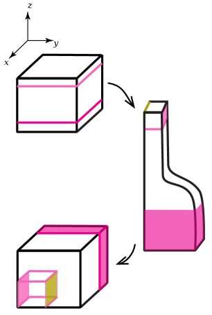
We start describing the family of three dimensional horseshoes introduced by Díaz, Horita, Rios and Sambarino in [5].
Let be the cube in and consider the parallelepipeds:
The horseshoe map is defined on and as follows
where , and
Fig. 1. The function .
And
where and .
Then, for , we have
(1)
If but does not belong to or , then will be mapped injectively outside .
We point out that besides we refer simply to , we have described a family of maps that depends on the parameters and . We consider fixed parameters satisfying conditions above.
In figure 2 we see the steps of the construction of the horseshoe.
Fig. 2. The horseshoe
Let be the maximal invariant set under of the union of the parallelepipeds and :
In [5] it was shown that the maximal invariant set is partially hyperbolic, with one dimensional central direction, parallel to the -axis. The central direction presents contractive and expanded behavior. The horizontal direction is contractive while the vertical direction, parallel to the -axis, is expanding.
The uniqueness of equilibrium states for the horseshoe associated to potentials with small variation was proved in [12]. The main goal of this work is to study the statistical behavior of this equilibrium. Here we state the result in [12]. Let .
Theorem 2.1.
Let be the three dimensional partially hyperbolic horseshoe defined above. Let be a Hölder continuous potential with . Assume that does not depend on the -coordinate in each set and . Then there exists a unique equilibrium state for the system with respect to the potential .
We consider potentials as above and additionally we assume that the Hölder constant of is small. The explicit condition will be stated in Section 4. We point out that this is an open condition which includes, for instance, constant potentials.
For the equilibrium state of the system we will establish exponential decay of correlations for Hölder continuous observables.
Theorem A.
The equilibrium state has exponential decay of correlations for Hölder continuous observables: there exists a constant such that for all there exists satisfying
We also derive a central limit theorem for the equilibrium state of the horseshoe with respect to a potential as considered above.
Theorem B.
Let be a Hölder continuous function and let
be defined by
Then is finite and if and only if for some . On the other hand, if then given any interval ,
as goes to infinity.
Now we describe a map that was defined in [12] which is related to the projection of on two center-stable planes. By an abuse of notation the map will be called the projection map. Besides the inherent interest in the dynamics of the map , understanding the statistical behavior of its equilibrium is the crucial ingredient in the proofs of Theorem A and Theorem B.
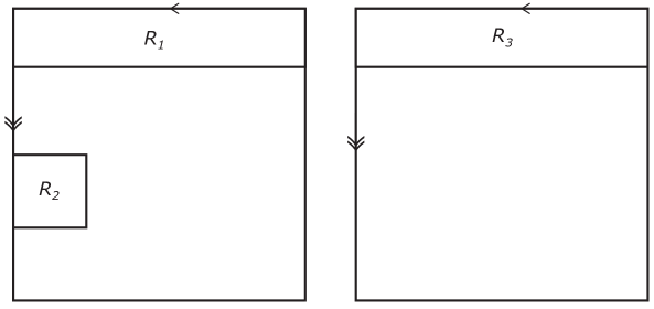
We define as follows the rectangles , and :
with close to zero.
Fig. 3. The rectangles , and .
The rectangles are inside two planes that we will call and (see figure 3). We consider an abstract space which is the union of the rectangles. Notice this is a metric space endowed with some natural metric , say the one, induced by .
Let be defined by and . Take .
Consider the map defined by its restrictions to each rectangle as follows:
Note that is uniform expanding while we have both, expanding and contracting, behaviors in and .
The map acts similarly on and . In these rectangles, the points are sent from the right side to the left, except for the extreme points whose coordinates are fixed.
Let be the maximal invariant set under of the union of the rectangles , and :
and from now on we denote simply by the restriction of to .
Let be the subshift of finite type
with transition matrix:
The following transitions are allowed:
Notice that is is not conjugated but only semi-conjugated to the shift . That is because the entire segment is associated to the constant sequence on .
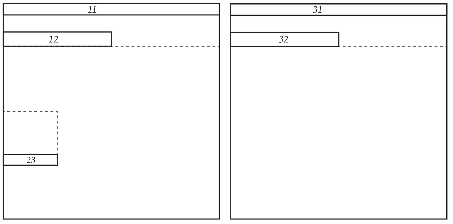
We point out that the 3-rd iterate of any rectangle covers .
Moreover, is topologically mixing.
Note that points belonging to the rectangles 1 and 2 have two pre-images, while points in the rectangle 3 have just one pre-image.
Fig. 4. Second generation
Fig. 5. Third generation
Figure 5 and figure 5 show the first steps in the generation of the set . Since contains infinitely many line segments it is not a Cantor set.
The topological entropy of the subshift is given by:
Since and are semiconjugated we obtain .
In [12] it was shown the uniqueness of equilibrium states associated to Hölder continuous potentials satisfying
. In this work we consider potentials as above and assume an additional condition that will be stated in Section 4. For the system we obtain some statistical properties of its equilibrium measure . As mentioned before, these results will be used to derive the statistical properties of the equilibrium of the horseshoe announced above.
The following result states the exponential decay of correlations for Hölder continuous observables.
Theorem C.
There exists a constant such that for all and there exists satisfying
We also obtain a central limit theorem for the equilibrium.
Theorem D.
Let be a Hölder continuous function and let be defined by
Then is finite and if and only if for some . On the other hand, if then given any interval ,
as goes to infinity.
2.1. Ruelle-Perron-Frobenius operator and its spectral gap
Let be the system defined above. Denote by the set of real continuous functions on . We define the operator called the Ruelle-Perron-Frobenius operator or simply the transfer operator, which associates to each a continuous function
by:
The transfer operator is a positive bounded linear operator.
For each we have
where denotes the Birkhoff sum .
We also consider the dual operator that satisfies
for every and every .
We will state here for further reference an important property for the transfer operator and its dual which was obtained in [12].
Theorem 2.2.
Let be the spectral radius of the transfer operator . There exist a probability measure and a Hölder continuous function bounded away from zero and infinity which satisfies
We point out that the unique equilibrium state associated to the system is given by .
The Ruelle-Perron-Frobenius operator is said to have the spectral gap property if its spectrum can be decomposed as follows: where is an eigenvalue for associated to a one-dimensional eigenspace and is strictly contained in the ball .
Theorem E.
The Ruelle-Perron-Frobenius operator has the spectral gap property restrict to the space of Hölder continuous observables.
3. Invariant cones and projective metrics
The theory of projective metrics on convex cones and positive operators on a vector space is due to Birkhoff [1] and has been extensively studied (see [2] and [10]). Projective metrics associated to cones provide an elegant way to express spectral properties of the transfer operator.
In this section we will state some results regarding this theory in order to prove the spectral gap of the transfer operator.
Let be a Banach space. A subset of is called a cone in if it is a convex space which satisfies:
1)
2)
We say that a cone is closed if .
Let be a closed cone and given define
(2)
We point out that is finite, is positive and for all .
We set
with possibly infinity in the case or .
It is straightforward to check that is well-defined and takes values in . Since we have that defines a pseudo-metric on . Then induces a metric on a projective quotient space of called the projective metric of .
Note that the projective metric depends in a monotone way on the cone: if are two cones in , then we have
where and are the projective metrics in and respectively.
Moreover, if is a linear operator and are cones in respectively, satisfying then
However is not necessarily a strict contraction, that will be the case for instance if had finite diameter in . This will be stated in the following result which is a key tool to prove the spectral gap for the Ruelle-Perron-Frobenius operator.
Proposition 3.1.
Let and be closed convex cones in the Banach spaces and respectively. If is a linear operator satisfying and then
For the proof of the last proposition see for example [[15], Proposition 2.3].
Next we will define a cone in the space of positive continuous functions. We start by recalling some definitions.
Let be an -Hölder continuous function and denote by
the Hölder constant of .
Given we say that a function is -Hölder continuous in balls of radius if for some constant we have for all .
We will denote by the smallest Hölder constant of in balls of radius .
We consider the space of -Hölder continuous observables endowed with the norm .
Consider the union of the rectangles , and and fix . Let be a
-Hölder continuous function in balls of radius . Then is -Hölder continuous in balls of radius for each
Indeed, fixing and given with , there exists such that and . Hence,
(3)
The next result states that every locally Hölder continuous function defined on is Hölder continuous.
Lemma 3.2.
Let and let
be a -Hölder continuous function in balls of radius . Then there exists such that is -Hölder continuous.
Proof.
By the compactness of , there exists which depends only on such that given there are with for all and
Since is -Hölder continuous in balls of radius it follows that
Thus is -Hölder continuous where .
∎
Now we consider the cone of locally Hölder continuous observables defined on :
(4)
It follows by definition that if .
Given an arbitrary we have . Moreover, by Lemma 3.2, is Hölder continuous with constant . Then
(5)
In the next lemma we give another expression for the projective metric on the cone , that we denote by and use in further estimates.
Lemma 3.3.
The metric in the cone is given by where
and
Proof.
First recall the definition of the projective metric and consider and as in equation (2). Let . Let be the supremum of positive numbers satisfying
.
This is equivalent to saying that for all and . Hence
(6)
Suppose that the minimum can be attained by the first term on the right side of the inequality. In this case, we can take satisfying
Thus, for every we have
This guarantees that the minimum in equation (6) is always attained by the right-hand side. To end the proof just notice that a similar computation can be done to get the expression for .
∎
4. Spectral gap
Consider the system where is the projection map defined in Section 2 and is a Hölder continuous potential with variation smaller than . We also assume that satisfies
(7)
Let be the transfer operator of associated to the potential . When there is no risk of confusion we will denote simply by .
Here we prove that the transfer operator has the spectral gap property on the space of Hölder continuous observables.
As mentioned in Section 2, the map is not injective on but it is injective when restricted to each of the rectangles , and . Moreover, for each . We will explore this property in order to construct a partition of such that the distance between pre-images under of points in the same element of the partition can be controlled.
Lemma 4.1.
There exists a finite cover of by injective domains of such that every has at most one pre-image in each element of the cover . Moreover, for we have that implies
where are pre-images of under belonging to the same element of .
Proof.
Let be the union of the rectangles and consider the partition . Thus is a finite cover of with elements and satisfies that is injective in each , .
Let . Given with we have, in particular, that belong to the same rectangle , .
Since and there is no loss of generality in assuming that . Let and . Let be the pre-images in the element . We have
Since preserves horizontal and vertical lines and contracts vertical lines we may assume that are on the same horizontal line. Again, using that the derivative in can be estimated by , it is straightforward to check that
Since we have .
∎
From now on we fix as in Lemma 4.1. Given let be the cone of locally Hölder continuous functions defined in equation 4. The next result states the strict invariance of the cone under the operator for large enough.
Proposition 4.2.
There exists such that
Proof.
Let and take with constant . Since is a positive and bounded operator we have that is a continuous and positive function. In order to prove the result we should find such that
Notice that given we have and thus
Considering with we have that belong to the same rectangle and, in particular, they have the same number of pre-images. So we can group the pre-images that are in the same rectangle. Thus
Observe that in the fourth inequality we used equation (3) and in the fifth inequality we applied equation (5).
By condition (7) we obtain that the last inequality is smaller than for some positive constant .
∎
The invariance of the cone is not enough to guarantee that the operator is a contraction. In order to prove this we have to verify that the cone given by the previous proposition has finite diameter.
Proposition 4.3.
The cone has finite diameter for sufficiently large.
Since and are arbitrary it implies that the diameter of is finite.
∎
Combining Proposition 4.2 and Proposition 4.3 we are able to apply Proposition 3.1 to establish the next result.
Proposition 4.4.
The operator is a contraction in the cone : for the constant we have
As in Subsection 2.1 we consider the function and the measure satisfying and . Also recall that . From the last proposition we will derive exponential convergence of the transfer operator to the eigenfunction in the space of Hölder continuous observables.
Proposition 4.5.
For every satisfying there exist some positive constant and such that
Proof.
Let with . Since is the reference measure associated to and we have for every
Thus, for every we derive
Let and where
. From Lemma 3.3 and Proposition 4.4 we have
Now, given write with and . Since is a bounded operator and , we conclude that
∎
As a consequence of the exponential convergence we can prove the following property of the equilibrium state associated to the system .
Corollary 4.6.
The sequence of push forwards of the reference measure converges to the equilibrium state .
Proof.
Let be arbitrary. Since we have
By Proposition 4.5 the sequence converges uniformly to which implies
and ends the proof.
∎
To finish this section we prove the spectral gap of the transfer operator.
Theorem 4.7.
The operator acting on the space admits a decomposition of its spectrum: there exists such that with contained in a ball centered at zero and of radius .
Proof.
Consider .
Define and as the eigenspace associated to the eigenvalue . Notice that .
We can decompose as a direct sum of and . In fact, given write
and notice that belongs to and belongs to since .
Thus in order to derive the spectral gap for in it is enough to prove that is a contraction in for sufficiently large.
We take large enough such that the cone is preserved by .
Take with . So does not necessarily belong to the cone but since
To complete the proof it is enough to observe that the spectrum of is given by where is the spectrum of .
∎
5. Statistical behavior for the equilibrium of the projection map
In this section we will prove Theorem C and Theorem D. The exponential convergence of the transfer operator to the invariant density in the space of Hölder continuous observables will allow us to establish an exponential decay of correlations for the equilibrium state of .
Theorem 5.1.
The equilibrium state associated to the system has exponential decay of correlations for Hölder continuous observables: there exists such that for all and there exists a positive constant satisfying:
Proof.
Recall that , the eigenfunction of the transfer operator associated to the spectral radius , is bounded away from zero and infinity. Let us consider first the case for large enough. Without loss of generality, suppose
. Thus we have
By Proposition 4.5 there exists a positive constant such that
In the general case fix and write
where
Hence and we can apply the previous estimates to By linearity the proposition holds.
∎
We point out that since the transfer operator converges to the density in the space of Hölder continuous observables, we can estimate the constant obtained in the last proposition as follows
(10)
where the constant does not depend on or on and is a constant that depends only on .
Let be the Borel -algebra of and denote for . A real function is -measurable if and only if there exists a -measurable function satisfying . Moreover, we have the decreasing inclusion: .
Let be the intersection
An invariant probability measure is said to be exact if every -measurable function is constant - almost everywhere.
As a first consequence of the exponential decay of correlations we obtain the exactness property of the equilibrium measure associated to the system .
Corollary 5.2.
The equilibrium state is exact.
Proof.
Given a -measurable function, for each there exists a -measurable function such that . In particular, . By the decay of correlations, Theorem C, combined with (10) for any Hölder continuous function there exists such that
Since the last term converges to zero when goes to infinity we have
Since is arbitrary it follows that is constant -almost everywhere.
∎
Notice that, in particular, the exacteness of implies its ergodicity.
In order to establish a central limit theorem for the equilibrium state of we first state a non-invertible case of an abstract central limit theorem due to Gordin. For its proof one can see e.g. [[15], Theorem 2.11].
Theorem 5.3(Gordin).
Let be a probability space and be a measurable map such that is an invariant ergodic probability measure. Let such that . Denote by the non increasing sequence of -algebras and assume
Then given by
is finite and if and only if for some . On the other hand, if then given any interval ,
as goes to infinity.
Now we derive from this result Theorem D.
For each denote by the set . We have a sequence of inclusions .
Since is a Hilbert space, given denote by the orthogonal projection of to .
Let be a Hölder continuous function such that , then for all we have
Note that in order to obtain the first inequality we apply the exponential decay of correlations from Theorem C. We warn the reader that when applying Theorem C, plays the role of while plays the role of . To get the last inequality we used that .
Therefore the series is summable.
Applying Theorem 5.3 we get a central limit theorem for the equilibrium state of . This proves Theorem D.
6. Statistical properties for equilibrium of horseshoes
In the last section we have shown that the existence of a spectral gap for the transfer operator associated to the system implies an exponential decay of correlations for the equilibrium on the space of Hölder continuous observables. Moreover, we also derived a central limit theorem for that equilibrium.
In this section we will use these results to derive similar statistical properties for the equilibrium state associated to the horseshoe defined in Section 2. We point out that since is a diffeomorphism we can consider its inverse and from the way that we have defined the projection map we will state the results for .
The key idea in this section is to disintegrate the equilibrium state for the horseshoe as a product of the equilibrium state for the system and conditional measures on the stable fibers. For this we will use the following result due to Rohlin [13]. The formulation stated here was given in [14].
Theorem 6.1(Rohlin’s Disintegration Theorem).
Let X and Y be metric spaces, each of them endowed with the Borel -algebra. Let be a probability measure on , let be measurable and let . Then there exists a system of conditional measures of with respect to , meaning that
1)
is a probability measure on X supported on the fiber for -almost every .
2)
the measures satisfy the law of total probability
for every Borel subset of .
These measures are unique in the sense that if is any other system of conditional measures, then for -almost every .
We point out that the conditional measures system in the last theorem is given by the weak∗ limit:
where is the conditional probability relative to . Notice that is supported entirely on the fiber .
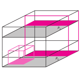
In order to relate and we consider a projection of the parallelepipeds and onto the planes and . See figure 6.
Fig. 6. Horizontal planes
Define by
Note that for each plane we have that .
It is straightforward to check that is continuous, surjective and
Thus is a semiconjugacy between and .
Let be a H lder continuous potential that does not depend on the -coordinate, i.e., is a constant function for every fixed. Hence induces a H lder continuous potential defined on by
(11)
which has the same variation as .
In [12] it was proved that when the variation of is smaller than there exists a unique equilibrium state associated to the horseshoe. Moreover, denoting by the equilibrium state of where is given by (11) this measure is the push-forward by of . In other words for every Borel set of the -algebra on we have
Recall that here the potential also satisfies condition (7).
Consider the projection in the third coordinate .
Applying Rohlin’s theorem we have for every Borel subset of
where is the system of conditional measures for the disintegration of with respect to .
In the next lemma we relate this system with the equilibrium state of the projection map.
Lemma 6.2.
Given and a Borel subset of we have
Proof.
Fixing and given we have that is a subset of the plane . Therefore
∎
Now we are able to prove the exponential decay of correlations for the equilibrium state associated to the horseshoe.
Theorem 6.3.
The probability measure has exponential decay of correlations for Hölder continuous observables: there exists such that for every and there exists such that
Proof.
Let and such that . For each using Lemma 6.2 we have
Note that for each fixed is a Hölder continuous function on and . Also, belongs to . Then by the exponential decay of correlations property of , Theorem C, there exists a positive constant and such that
where is a uniform bound (in ) for obtained from equation (10).
We proved the desired inequality when satisfies . For the general case it is enough to observe that
This ends the proof.
∎
Using equation (10) and the -invariance of the equilibrium we can prove Theorem A from the last result:
Since we have showed exponential decay of correlations for the equilibrium state it is straightforward to check that the same steps of the proof of exactness for the equilibrium associated to projection map (Corollary 5.2) hold in this context.
Corollary 6.4.
The equilibrium state is exact.
Finally consider the Borel -algebra of and the decreasing sequence defined by for every Let be a Hölder continuous function satisfying Using the exponential decay of correlations of we obtain that the series is summable, where is the orthogonal projection of to for each .
Applying Gordin’s theorem we deduce that a central limit theorem holds for Thus we have finished the proof of Theorem B.
Acknowledgments
This work was carried out at Universidade do Porto. The authors are very thankful to Silvius Klein for the help with the manuscript version and encouragement. VR is grateful to Ivaldo Nunes for the encouragement.
References
[1] Birkhoff, G. Lattice Theory American Mathematical Society Colloquium Publications 25 (4th ed.), Providence, R.I.: American Mathematical Society, (1979).
[2] Baladi, V., Positive Transfer Operators and Decay of Correlations World Scientific Publishing Co. Inc. (2000).
[3] Castro, A., Nascimento, T., Statistical properties of the maximal entropy measure for partially hyperbolic attractors Erg. Theory and Dyn. Sys. Available on CJO2016. doi:10.1017/etds.2015.86.
[4] Castro, A., Varandas, P., Equilibrium states for non-uniformly expanding maps: decay of correlations and strong stability Annalles de l’Institut Henri Poincaré - Analyse Non-Linéaire, 225-249, (2013).
[5] Díaz, L., Horita, V., Rios, I., Sambarino, M., Destroying horseshoes via heterodimensional cycles: generating bifurcations inside homoclinic classes, Ergodic Theory and Dynamical Systems, 29 (2009) pp 433-474.
[6] Dürr, D., Goldstein, S., Remarks on the central limit theorem for weakly dependence random variables Stochastic processes - mathematics and physics, Lect. Notes in Math., Vol 1158, Springer Verlag, Berlim, (1986) pp 104-118.
[8] Keller, G. Un theorème de la limite centrale pour une classe de tranformations monotones par morceaux C.R.A.S. A 291 (1980), pp 155-158
[9] Keller, G., Nowicki, T.,Spectral theory, zeta functions and the distribution of periodic points for Collet-Eckmann maps Comm. Math. Phys. (1992) 149, pp 31-69.
[10] Liverani, C. Decay of correlations Ann. of Math. 142 (1995) pp 239-301.
[11] Liverani, C. Decay of correlations for piecewise expanding maps J. Stat. Phys. 78 (1995) 1111-1129.
[12] Rios, I., Siqueira, J., On equilibrium states for partially hyperbolic horseshoes, Ergodic Theory and Dynamical Systems,
[13] Rohlin, V. A., On the fundamental ideas of measure theory, Amer. Math. Soc. Translation,
(1952). no. 71, pp 55 .