On the average of electrostatic and magnetostatic fields, the singularities of dipole fields and depolarizing fields

In [1] it is proved that the average of the electrostatic field taken over a spherical volume equals the electric field at the center of the sphere if the charge distribution causing the field is completely located outside the sphere. If on the other hand the charge distribution is completely enclosed by the sphere then the average is proportional to the elecric dipole moment of the charge distribution calculated with respect to the center of the sphere. The proof of this property is based on an expansion in spherical harmonics of the potential of a monopole and similar results hold for magnetostatic fields. The second form of the theorem has then be used to derive the singularity of the electric/magnetic dipole fields, which has received some attention recently [2, 3].

In §2-3 we will show that both theorems can be proved rather easily by invoking the reciprocity of the fields and especially for the electrostatic case (§2) the derivation is almost immediate. In §3 the corresponding magnetostatic theorem is proved using the conventional current loop model for a magnetic dipole. In §4 we briefly recall how the singularities of the dipole fields can be found using these theorems. In §5 the close link is revealed between these singularities and the well-known depolarizing field of a sphere. This also enables us to extend the results to more general shapes of the volume and finally in §6 to an anisotropic background medium.

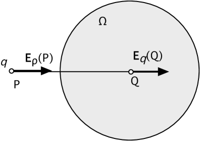
It is of course sufficient to prove the theorem for the field of a single monopole q. Using superposition the extension to an arbitrary charge distribution is then straightforward. We thus consider the average of the field of a monopole $q$, located at P, over a spherical volume $\Omega$ (see figure 1). Using reciprocity we conclude that the average field $\left\langle\overline{E}_{q}\right\rangle_{\Omega}$ equals the field $\overline{E}_{\rho}(\mathrm{P})$ at the source point P generated by a charge $-q$ uniformly distributed over the volume $\Omega$ with density $\rho=-q/|\Omega|$, where $|\Omega|$ is the size of this volume. This first step in the reasoning is valid for an arbitrary volume. For a spherical volume with center at Q the latter field is easily calculated. If the source point P is outside the sphere ($\mathrm{P}\notin\Omega$) then $\overline{E}_{\rho}(\mathrm{P})$ equals the field of a single monopole $-q$ at the center Q of the sphere and applying reciprocity again it follows that the averaged field equals the field of the original charge q measured at the center of the sphere:

$$\left\langle\overline{E}_{q}\right\rangle_{\Omega}=\overline{E}_{\rho}(\mathrm{P})=\overline{E}_{-q}(\mathrm{P})=\overline{E}_{q}(\mathrm{Q})\qquad\mathrm{P}\notin\Omega$$

(1)

The two outer equalities are due to reciprocity, the central one is due to the spherical symmetry.

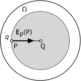
If on the other hand the source point is enclosed by the sphere ($\mathrm{P}\in\Omega$) then invoking again the spherical symmetry a standard application of Gauss integral law yields:

$$\left\langle\overline{E}_{q}\right\rangle_{\Omega}=\overline{E}_{\rho}(\mathrm{P})=-\frac{q\overline{\mathrm{QP}}}{3\varepsilon_{0}|\Omega|}=-\frac{\bar{p}_{q}}{3\varepsilon_{0}|\Omega|}\qquad\mathrm{P}\in\Omega$$

(2)

where $\overline{p}_{q}$ is the dipole moment of $q$ with respect to the center of the sphere.

A similar reasoning can be followed for the magnetostatic case, although the calculations are slightly more complicated if the conventional electric-current model is used for the magnetic dipole ($\overline{m}=i\bar{a}$ with i the current in the loop and $\overline{a}$ the oriented area of the loop). The magnetostatic result can be obtained much more economically by using the magnetic-charge model [4] instead (see §4). However since the current model is more widely adopted and for completeness we show the derivation for this model too.

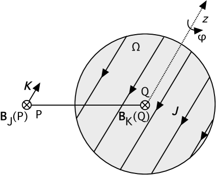
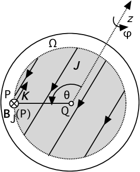
We consider a $\delta$-like current element which we denote by $\overline{K}$ (with the current density $\bar{J}(\bar{r})=\overline{K}\delta(\bar{r}-\bar{r}_{\mathrm{P}})$). Without loosing generality we choose the origin at the center Q of the sphere and the z-axis along the direction of $\overline{K}$ with $\overline{K}=K\overline{1}_{z}$ (see figure 2). Using the reciprocity of Biot-Savart’s law the magnetic induction $\left\langle\overline{B}_{\bar{K}}\right\rangle_{\Omega}$ of the current element at P averaged over the sphere $\Omega$ equals the induction $\overline{B}_{\bar{J}}(P)$ measured at P of a uniform current density $\overline{J}=-\overline{K}/|\Omega|$ present in the sphere. The solution of the latter problem is analogous with the electrostatic problem with the correspondence $q/\varepsilon_{0}\leftrightarrow\mu_{0}K$ and $E_{r}\leftrightarrow B_{\varphi}/\sin\theta$ where $E_{r}=-d\phi/dr$ is the radial electrostatic field and $B_{\varphi}=-\sin\theta dA_{z}/dr$ the tangential component of the induction, $\phi$ being the electrostatic potential and $\overline{A}=A_{z}\overline{1}_{z}$ the vector potential, and where $\theta$ is the angle between the $z$-axis and the position vector $\overline{r}$. It then follows readily that:

$$\left\langle\overline{B}_{\bar{K}}\right\rangle_{\Omega}=\overline{B}_{\bar{J}}(\mathrm{P})=\bar{B}_{-\bar{K}}(\mathrm{P})=\overline{B}_{\bar{K}}(\mathrm{Q})\quad\mathrm{P}\notin\Omega$$

(3)

for the situation in figure 2(a) and for the situation in figure 2(b) we find similarly:

$$\left\langle\overline{B}_{\bar{K}}\right\rangle_{\Omega}=\overline{B}_{\bar{J}}(\mathrm{P})=-\frac{\mu_{0}K}{3|\Omega|}|\overline{\mathrm{PQ}}|\sin\theta\overline{1}_{\varphi}=-\frac{\mu_{0}}{3|\Omega|}\overline{\mathrm{PQ}}\times\overline{K}=\frac{2\mu_{0}}{3|\Omega|}\overline{m}_{\bar{K}}\quad\mathrm{P}\in\Omega$$

(4)

where $\overline{m}_{\bar{K}}$ is the magnetic moment of the current element with respect to the center Q of the sphere. Note that the extra factor 2 compared with the electrical dipole is due to the factor 1/2 in the definition of the magnetic moment, this being a second order moment, whereas the electric dipole moment is of first order. The results (3) and (4) are again easily extended for an arbitrary current density distribution $\overline{J}(\overline{r})$.

Applying the second form of the theorem (2) to the field of a dipole $\bar{p}$ enclosed by an arbitrary sphere it follows that the field must contain a singularity $-\frac{\bar{p}}{3\varepsilon_{0}}\delta(\bar{r})$. To take this singularity into account the field is then written explicitly as [1]:

$$\varepsilon_{0}\overline{E}_{\overline{p}}=\frac{\overline{p}}{4\pi}\cdot\frac{3\overline{r}\overline{r}-r^{2}\overline{\overline{I}}}{r^{5}}-\frac{\overline{p}}{3}\delta(\overline{r})$$

(5)

where $\overline{\overline{I}}$ is the unit tensor and where we have written the field in a form which is more amenable to a generalization to anisotropic media (see §6). The interpretation of this expression requires some care. If the sphere is centered on the dipole then the average of the first non-singular term vanishes only if one excludes an infinitesimal spherical volume around the dipole. This actually means that (5) is only valid if the dipole is modelled as an infinitesimally small polarized sphere, as will become more explicit in §5. As an additional bonus we find that, since the average of the field is, according to (2), independent of the position of the dipole within the sphere, the principal value integral of the first term must also vanish if the sphere is not centered on the dipole.

The corresponding magnetostatic result can be obtained immediately by using the magnetic-charge model [4] for the magnetic dipole. In this model a magnetic moment is composed of 2 magnetic charges $\pm\,q^{*}$ a distance $\overline{d}$ apart. Then $\mu_{0}\overline{m}=q^{*}\overline{d}$ and due to the analogy with the electrostatic case the magnetic field $\overline{H}$ will show a singularity $-\frac{\overline{m}}{3}\delta(\bar{r})$. Since $\overline{B}/\mu_{0}=\overline{H}+\overline{M}$ and $\overline{M}=\overline{m}\delta(\bar{r})$ it follows that $\overline{B}/\mu_{0}$ must have a singularity $\frac{2}{3}\bar{m}\delta(\bar{r})$ which agrees with (4) found higher. Finally we note that for the electrostatic case the electric induction $\bar{D}$ also shows a singularity $\frac{2}{3}\overline{p}\delta(\overline{r})$.

Applying the theorem in (1) once more to a dipole¹¹1In what follows we limit ourselves to the electrostatic case, but all results are readily extended to the magnetic case. $\bar{p}$ we find that the field of a dipole averaged over a sphere (not enclosing the dipole) is equal to the field of the same dipole measured at the center of the sphere. Applying reciprocity to both sides of this equality it follows that the (external) field of a uniformly polarized sphere ($\overline{P}=\overline{p}/|\Omega|$) is equal to the field of a dipole $\bar{p}$ at its center. The same reasoning can be applied for any higher order multipole. Similarly applying (2) for a dipole but now enclosed by the sphere it follows that the electric field within a uniformly polarized sphere ($\overline{P}=\overline{p}/|\Omega|$) is uniform and equal to $-\frac{\overline{P}}{3\varepsilon_{0}}$. This is the well-known depolarizing field of a sphere which is thus shown to be directly related to the singularity in (5) and this leads us to the conclusion that (5) is only valid if the dipole is modelled as an infinitesimally small polarized sphere. Applying the same reasoning to any higher-order multipole and since the dipole moment of any higher-order multipole vanishes we conclude that in a sphere filled with a uniform higher-order multipole density the internal field vanishes.

These results can be formalized as follows. Using the same notation as before the field of a multipole averaged over an arbitrary volume $\Omega$ can be found by filling $\Omega$ with a corresponding multipole density and looking for the field at the source point P:

	$\displaystyle\left\langle\overline{E}_{q}\right\rangle_{\Omega}$	$\displaystyle=\overline{E}_{\rho}(\mathrm{P})$
	$\displaystyle\left\langle\overline{E}_{\overline{p}}\right\rangle_{\Omega}$	$\displaystyle=\overline{E}_{\overline{P}}(\mathrm{P})$		(6)
	$\displaystyle\left\langle\overline{E}_{\overline{\overline{q}}}\right\rangle_{\Omega}$	$\displaystyle=\overline{E}_{\overline{\overline{Q}}}(\mathrm{P})$
		$\displaystyle\ldots$

where $\rho=-q/|\Omega|$, $\overline{P}=\overline{p}/|\Omega|$, $\overline{\overline{Q}}=-\overline{\overline{q}}/|\Omega|$, … are the charge density, polarization density and quadrupole density, … corresponding with the charge $q$, the dipole $\overline{p}$, the quadrupole $\overline{\overline{q}}$ … . The multipole fields on the left sides follow from each other by differentiation:

	$\displaystyle\overline{E}_{\overline{p}}$	$\displaystyle=-\overline{p}\cdot\nabla\overline{E}_{q}/q$
	$\displaystyle\overline{E}_{\overline{\overline{q}}}$	$\displaystyle=\overline{\overline{q}}\cdot\nabla\nabla\overline{E}_{q}/q$		(7)
		$\displaystyle\ldots$

Due to reciprocity similar relations hold for the fields on the right sides:

	$\displaystyle\overline{E}_{\overline{P}}$	$\displaystyle=-\overline{P}\cdot\nabla\overline{E}_{\rho}/\rho$
	$\displaystyle\overline{E}_{\overline{\overline{Q}}}$	$\displaystyle=\overline{\overline{Q}}\cdot\nabla\nabla\overline{E}_{\rho}/\rho$		(8)
		$\displaystyle\ldots$

with $\nabla$ operating on the position vector of the (original) source point $\mathrm{P}$. Note that (6) and (8) are valid for arbitrary volumes. The field of a uniformly polarized body in particular can thus be derived from the field of the same uniformly charged body. This method for calculating the field of a uniformly polarized (or magnetized) volume has been attributed to Poisson [5].

For a sphere in addition the symmetry can be invoked and the external field of a uniformly charged sphere simply equals that of a monopole. Therefore the field of a uniformly polarized sphere also equals a dipole field and similar results hold for higher order multipole moments. Since the internal field of a uniformly charged sphere is linear in the position, as shown in (2), the internal field of a uniformly polarized sphere is then according to the first equation in (8), a constant and given by:

$$\left\langle\overline{E}_{\overline{p}}\right\rangle_{\Omega}=-\frac{\bar{p}}{3\varepsilon_{0}|\Omega|}=-\frac{\overline{P}}{3\varepsilon_{0}}=\overline{E}_{\overline{P}}(\mathrm{P})\qquad\mathrm{P}\in\Omega$$

(9)

where we stress once again the relation between the singularity of the dipole field on the left and the depolarizing field of a uniformly polarized sphere on the right. Due to the linear dependence on the position vector it follows immediately that the internal field vanishes for all higher-order uniform multipole densities.

Having found this relation it becomes straightforward to look for extensions of the theorems (1) and (2) to other than spherical volumes. It is obvious that an extension to ellipsoidal volumes must be possible for an internal point. Therefore we consider firstly a (centric) hollow sphere. From the linear position dependence in (2) it is clear that the averaged electric field of any charge enclosed by the hollow sphere is zero and this is equivalent with the well-known property that the field of a uniformly charged hollow sphere is zero in the enclosed space. It also readily follows that this remains true for an enclosed dipole distribution (and for the corresponding polarized hollow sphere) even if the inner sphere is eccentric. This argument can be reversed as follows. If the electric field in a uniformly charged (centric) hollow sphere vanishes within the enclosed space then the internal electric field of a uniformly charged (single) sphere must be linear dependent on the position. Indeed if the latter field (say of the outer sphere) is denoted by $\overline{E}(\overline{r})$, with the origin taken at the center, then in the enclosed space of a hollow sphere the field equals $\overline{E}(\overline{r})-s\overline{E}(\overline{r}/s)$, where s is the scale factor scaling the outer sphere to the inner one. If this field vanishes then $\overline{E}(\overline{r})$ must be linear in $\overline{r}$.

Next we transform a spherical shell into a more general ellipsoidal shell by directional scaling. Taking into account the quadratic dependence of the electric field on distance it is easy to show that also in the cavity of a uniformly charged hollow ellipsoid²²2By a hollow ellipsoid we mean that inner and outer bounding surfaces are similar ellipsoids, which should not be confused with the case that the ellipsoids are confocal. the field vanishes [6]. Therefore applying the same scaling argument as above, the internal field of a uniformly charged ellipsoid is also linear in the position (referred to the center) and (2) can then be written for an arbitrary ellipsoid as:

$$\left\langle\overline{E}_{q}\right\rangle_{\Omega}=\overline{E}_{\rho}(\mathrm{P})=-\frac{q}{\varepsilon_{0}|\Omega|}\overline{\overline{L}}_{i}\cdot\overline{\mathrm{QP}}=-\overline{\overline{L}}_{i}(\overline{\overline{A}})\cdot\frac{\overline{p}_{q}}{\varepsilon_{0}|\Omega|}\qquad\mathrm{P}\in\Omega$$

(10)

Where $\overline{\overline{L}}_{i}$ depends on the shape of the ellipsoid, defined by $\overline{\overline{A}}:\overline{r}\overline{r}=1$, $\overline{\overline{A}}$ being a symmetric positive definite tensor, and the index $i$ refers to “isotropic” since we are still considering an isotropic background. Using (8) it follows that:

$$\left\langle\overline{E}_{\overline{p}}\right\rangle_{\Omega}=\overline{E}_{\overline{P}}(\mathrm{P})=-\overline{\overline{L}}_{i}(\overline{\overline{A}})\cdot\frac{\overline{P}}{\varepsilon_{0}}\qquad\mathrm{P}\in\Omega$$

(11)

showing that $\overline{\overline{L}}_{i}$ is the usual depolarizing tensor. Of course one still needs a method for calculating this tensor. Today the best known approach is probably by the method “separation of variables” in ellipsoidal coordinates [7], but $\overline{\overline{L}}_{i}$ can also be calculated directly [8]. Perhaps the most elegant expression can be found by solving the problem in Fourier-space [9, 10]:

$$\overline{\overline{L}}_{i}(\overline{\overline{A}})=\frac{\overline{\overline{A}}}{4\pi}\cdot\int\frac{\overline{n}\overline{n}}{\overline{\overline{A}}:\overline{n}\overline{n}}d\Omega$$

(12)

where $\overline{n}$ is a unit vector in the (spatial) frequency space and the integration is over the surface of the unit sphere. The expression immediately reveals that the trace of the depolarizing tensor equals 1.

Now turning again to a hollow ellipsoidal shell it follows from (11) that the field is still zero if the inner ellipsoid becomes eccentric, but still aligned with the similar outer ellipsoid. This means that if such an eccentric hollow ellipsoid encloses a dipole, the average of the field over its volume vanishes. In particular the principal value integral of the dipole field over an ellipsoidal volume thus vanishes if the exclusion volume is a uniformly scaled version of the ellipsoid and irrespective of the position of the dipole³³3In an appendix of [11] this is proved directly and from this the constancy of $\overline{\overline{L}}_{i}$ is derived.. The corresponding singularity of the dipole field is then $-\overline{\overline{L}}\cdot\frac{\overline{p}}{\varepsilon_{0}}\delta(\overline{r})$ and more in general (5) is written as:

$$\varepsilon_{0}\overline{E}_{\overline{p}}=\frac{\overline{p}}{4\pi}\cdot\frac{3\overline{r}\overline{r}-r^{2}\overline{\overline{I}}}{r^{5}}-\overline{\overline{L}}_{i}(\overline{\overline{A}})\cdot\overline{p}\delta(\overline{r})$$

(13)

In this case the dipole is thus modelled more generally as an infinitesimally small ellipsoid. Obviously there is no unique singularity for a dipole field and the singularity depends on the symmetry attributed to the dipole.

The “external” theorem (1) cannot be extended from a spherical body to an ellipsoidal body since the field outside a uniformly charged ellipsoid is not longer equal to that of a monopole, because the even order multipole moments do not vanish. Consequently the field outside a uniformly polarized ellipsoid is also not longer equal to a pure dipole field. However if the ellipsoid is made infinitesimally small, preserving the shape and keeping the dipole moment constant, then all higher order moments of the uniform charge distribution will vanish and the external field of the polarized body once more becomes a pure dipole field, independent of the shape of the ellipsoid. This explains why the non-singular part in (13) does not depend on the shape.

The results can also be extended to a uniform anisotropic background medium. E.g. consider a uniform dielectric medium with symmetrical relative dielectric tensor $\overline{\overline{\varepsilon}}$. The extension is easily handled by introducing a suitable coordinate transformation which transforms the anisotropic medium into an isotropic one and then applying the results for the isotropic medium [12]. If we preserve the electric potential and charge density in corresponding points then the relevant transformation formulas are given by:

	$\displaystyle\overline{r}$	$\displaystyle=\overline{\overline{T}}^{1/2}\cdot\overline{r}^{\prime}$
	$\displaystyle\overline{E}$	$\displaystyle=\overline{\overline{T}}^{-1/2}\cdot\overline{E}^{\prime}$
	$\displaystyle\overline{D}$	$\displaystyle=\overline{\overline{T}}^{1/2}\cdot\overline{D}^{\prime}$
	$\displaystyle\overline{\overline{\varepsilon}}$	$\displaystyle=\overline{\overline{T}}^{1/2}\cdot\overline{\overline{\varepsilon}}^{\prime}\cdot\overline{\overline{T}}^{1/2}$
	$\displaystyle q$	$\displaystyle=|\overline{\overline{T}}|^{1/2}q^{\prime}$
	$\displaystyle\overline{p}$	$\displaystyle=|\overline{\overline{T}}|^{1/2}\overline{\overline{T}}^{1/2}\cdot\overline{p}^{\prime}$
	$\displaystyle\overline{\overline{A}}$	$\displaystyle=\overline{\overline{T}}^{-1/2}\cdot\overline{\overline{A}}^{\prime}\cdot\overline{\overline{T}}^{-1/2}$
	$\displaystyle\overline{\overline{L}}$	$\displaystyle=\overline{\overline{T}}^{1/2}\cdot\overline{\overline{L}}^{\prime}\cdot\overline{\overline{T}}^{-1/2}$		(14)

where $|\overline{\overline{T}}|$ is the determinant of $\overline{\overline{T}}$. With $\overline{\overline{T}}=\overline{\overline{\varepsilon}}$ the transformed dielectric tensor becomes isotropic ($\overline{\overline{\varepsilon}}^{\prime}=\overline{\overline{I}}$). Consider now as volume $\Omega$ an ellipsoid isomorphous with the “index ellipsoid” of the medium $\overline{\overline{\varepsilon}}^{-1}:\overline{r}\overline{r}=1$, then $\Omega$ is transformed into a sphere $\Omega^{\prime}$ in an isotropic medium, to which (1) can be applied. Transforming back we find that (1) remains valid for an anisotropic medium when applied to a volume isomorphous with the “index ellipsoid”. The depolarizing tensor $\overline{\overline{L}}(\overline{\overline{\varepsilon}},\overline{\overline{A}})$ depends on the anisotropy of the medium and on the shape of the ellipsoidal volume and follows directly from the last two transformation formula’s in (14):

$$\overline{\overline{L}}(\overline{\overline{\varepsilon}},\overline{\overline{A}})=\overline{\overline{\varepsilon}}^{1/2}\cdot\overline{\overline{L}}_{i}(\overline{\overline{\varepsilon}}^{1/2}\cdot\overline{\overline{A}}\cdot\overline{\overline{\varepsilon}}^{1/2})\cdot\overline{\overline{\varepsilon}}^{-1/2}$$

(15)

and (10) and (11) can thus be extended to:

	$\displaystyle\varepsilon_{0}\overline{\overline{\varepsilon}}\cdot\left\langle\overline{E}_{q}\right\rangle_{\Omega}$	$\displaystyle=-\overline{\overline{L}}(\overline{\overline{\varepsilon}},\overline{\overline{A}})\cdot\frac{\overline{p}_{q}}{|\Omega|}\qquad\mathrm{P}\in\Omega$		(16)
	$\displaystyle\varepsilon_{0}\overline{\overline{\varepsilon}}\cdot\left\langle\overline{E}_{\overline{p}}\right\rangle_{\Omega}$	$\displaystyle=-\overline{\overline{L}}(\overline{\overline{\varepsilon}},\overline{\overline{A}})\cdot\frac{\overline{p}}{|\Omega|}\qquad\mathrm{P}\in\Omega$

showing that the second theorem actually holds for the electric displacement instead of for the electric field. From (15) it also follows that the trace of $\overline{\overline{L}}(\overline{\overline{\varepsilon}},\overline{\overline{A}})$ is still 1.

As a special case we consider now a sphere ($\overline{\overline{A}}=\overline{\overline{I}}$) and we then obtain in particular $\overline{\overline{L}}(\overline{\overline{\varepsilon}},\overline{\overline{I}})=\overline{\overline{\varepsilon}}^{1/2}\cdot\overline{\overline{L}}_{i}(\overline{\overline{\varepsilon}})\cdot\overline{\overline{\varepsilon}}^{-1/2}=\overline{\overline{L}}_{i}(\overline{\overline{\varepsilon}})$ as given by (12) and where in the last step we used the property that $\overline{\overline{L}}_{i}(\overline{\overline{\varepsilon}})$ and $\overline{\overline{\varepsilon}}$ share the same principal axes. It follows that $\overline{\overline{\varepsilon}}$ and $\overline{\overline{A}}$ separately have the same effect on the depolarizing tensor. We consider then an alternative transformation which transforms the ellipsoid into a sphere ($\overline{\overline{T}}=\overline{\overline{A}}^{-1}$ and $\overline{\overline{A}}^{\prime}=\overline{\overline{I}}$) and obtain in this way an alternative expression for the depolarizing tensor:

$$\overline{\overline{L}}(\overline{\overline{\varepsilon}},\overline{\overline{A}})=\overline{\overline{A}}^{-1/2}\cdot\overline{\overline{L}}_{i}(\overline{\overline{A}}^{1/2}\cdot\overline{\overline{\varepsilon}}\cdot\overline{\overline{A}}^{1/2})\cdot\overline{\overline{A}}^{1/2}$$

(17)

The expression (17) with (12) has been further extended to a bianisotropic medium [13].

Comparing (15) and (17) it follows that:

	$\displaystyle\overline{\overline{L}}(\overline{\overline{\varepsilon}},\overline{\overline{A}})\cdot\overline{\overline{\varepsilon}}$	$\displaystyle=\overline{\overline{\varepsilon}}\cdot\overline{\overline{L}}(\overline{\overline{A}},\overline{\overline{\varepsilon}})$
	$\displaystyle\overline{\overline{A}}\cdot\overline{\overline{L}}(\overline{\overline{\varepsilon}},\overline{\overline{A}})$	$\displaystyle=\overline{\overline{L}}(\overline{\overline{A}},\overline{\overline{\varepsilon}})\cdot\overline{\overline{A}}$		(18)

showing the more general symmetry between anisotropy ($\overline{\overline{\varepsilon}}$) and shape ($\overline{\overline{A}}$). The non-singular part of the dipole field can also be obtained with the first coordinate transformation resulting into the following dipole field:

$$\varepsilon_{0}\overline{\overline{\varepsilon}}\cdot\overline{E}_{\overline{p}}=\frac{\overline{p}}{4\pi|\overline{\overline{\varepsilon}}|^{1/2}}\cdot\left[\frac{3\overline{\overline{\varepsilon}}^{-1}\cdot\overline{r}\overline{r}}{\left(\overline{\overline{\varepsilon}}^{-1}:\overline{r}\overline{r}\right)^{5/2}}-\frac{\overline{\overline{I}}}{\left(\overline{\overline{\varepsilon}}^{-1}:\overline{r}\overline{r}\right)^{3/2}}\right]-\overline{\overline{L}}(\overline{\overline{\varepsilon}},\overline{\overline{A}})\cdot\overline{p}\delta(\overline{r})$$

(19)

References

- [1] Jackson J D 1999 Classical Electrodynamics (New York: John Wiley & Sons) Ch 4
- [2] Leung P T and Ni G J Eur. J. of Phys. 27 (2006) N1-N3
- [3] Gsponer A Eur. J. of Phys. 28 (2007) 267-275
- [4] Fano R M, Chu L J and Adler R B 1960 Electromagnetic Fields, Energy, and Forces (New York: John Wiley & Sons)
- [5] Osborn J A Phys. Rev. 67 (1945) 351-357
- [6] Thomson W and Tait P G 1912 Treatise on natural philosophy, part II (Cambridge: At the University Press) §519
- [7] Landau L D, Lifshitz E M and Pitajevskii L P Electrodynamics of continuous media, 2nd edition (Elsevier Butterworth-Heinemann) §4
- [8] Reference [6] §494
- [9] Milton G W 2002 The theory of composites (Cambridge: Cambridge University Press) chapter 5
- [10] Michel B Int. J. of Applied Electromagnetics and Mechanics 8 (1997) 219-227
- [11] de Groot S R and Suttorp L G 1972 Foundations of electrodynamics (Amsterdam: North-Holland Publishing Company)
- [12] Sihvola A 2000 Electromagnetic mixing formulas and applications (The Institute of Electrical Engineers) 102
- [13] Weiglhofer W S (1999) ’Electromagnetic Field in theSource Region: A Review’, Electromagnetics, 19:6, 563 — 577
- [14] Weiglhofer W S “Depolarization Dyadics” Bianisotropics 2000 Sept. 27-29 415-420