On the behavior of a distributed network of capacitive constant phase elements

Now we consider the following distributed-order time differential equation [13, 25, 26, 15, 16] as a describing equation for a CPE network (compare with Eq. 1):

$$i(t)=\int_{\beta_{1}}^{\beta_{2}}\phi(\alpha)\,C_{\alpha}\,{}_{0}\text{D}_{t}^{\alpha}v_{c}(t)d\alpha$$

(6)

Here $\phi(\alpha)$ is a non-negative, time-invariant weight function defined on the interval $[\beta_{1},\beta_{2}]$ for $\alpha$, and acts as a (discrete or continuous) distribution of orders. The integral in Eq. 6 is known as a cumulative order distribution over the range of orders $\beta_{1}\leqslant\alpha\leqslant\beta_{2}$ [25], and is a direct generalization of the constant-order Caputo fractional derivative. For our purpose, we will restrict ourselves to the lower and upper values of the range of integration to zero and one (i.e. $0<\beta_{1}\leqslant\alpha\leqslant\beta_{2}<1$), which defines the spectrum going from an impedance of a pure resistor ($\alpha=0$) to that of a fractional capacitor ($0<\alpha<1$), to that of an ideal capacitor ($\alpha=1$). It is worth noting that Eq.  6 is one possible generalization of Eq. 1, amongst others, which can be used here to describe the current-voltage dynamics of more complex systems than a single-order CPE, such as heterogeneous electrode/electrolyte interfaces with multi-fractal properties [26]. A similar equation was studied for instance by Eab and Lim [26] for the case of simple free fractional Langevin equation without a friction term, i.e. with the left-hand side of Eq. 6 being a stationary Gaussian random noise. Lorenzo and Hartley also studied a similar problem of distributed order operators in the context of viscoelastic materials [25].

By applying the Laplace transform to Eq. 6, with the assumption of zero initial conditions, we obtain:

$$\tilde{i}(s)=\tilde{v}_{c}(s)\int_{\beta_{1}}^{\beta_{2}}\phi(\alpha)\,C_{\alpha}s^{\alpha}d\alpha$$

(7)

The corresponding impedance function is therefore:

$$\tilde{z}(s)=\left({\int_{\beta_{1}}^{\beta_{2}}\phi(\alpha)\,C_{\alpha}s^{\alpha}d\alpha}\right)^{-1}$$

(8)

and the time-domain voltage $v(t)$ can be found by the convolution integral:

$$v_{c}(t)=\int_{0}^{t}z(t-\tau)i(\tau)d\tau$$

(9)

where $z(t)=\mathcal{L}^{-1}\left[\tilde{z}(s);t\right]$.

The specific choice of $\phi(\alpha)$ in Eq. 6 depends on the underlying physics of the system under study. In what follows, we focus on two examples that can describe close enough what one may encounter when analyzing heterogeneous, complex electrodes in electrolytic media.

We first consider the case of a uniformly distributed order, i.e. a weight function $\phi(\alpha)$ given by:

$$\phi_{u}(\alpha)=\begin{cases}1,\;0\leqslant\alpha\leqslant 1\\ 0,\;\text{otherwise}\end{cases}$$

(10)

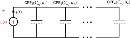
This means that the network (see Fig. 1) is composed of many elemental CPEs of different orders (taken from zero to one) while the value of $C_{\alpha}$ is the same for all CPEs; i.e. $C_{\alpha_{1}}=C_{\alpha_{2}}=\ldots=C_{\alpha_{n}}=C_{\alpha}$). The contributions of each and every elemental CPE are equally identical. Note that $\int_{0}^{1}\phi(\alpha)d\alpha$ does not need to be necessarily equal to one in this example, or in the general definition given above in Eq. 6 [27].

With the above assumptions, we obtain the overall network equivalent impedance as:

	$\displaystyle\tilde{z}_{u}(s)$	$\displaystyle=\left(C_{\alpha}{\int_{0}^{1}s^{\alpha}d\alpha}\right)^{-1}$
		$\displaystyle=\left(C_{\alpha}{\int_{0}^{1}e^{\alpha\ln(s)}d\alpha}\right)^{-1}=\frac{1}{C_{\alpha}}\frac{\ln(s)}{s-1}$		(11)

This result proves that the parallel association of CPEs with distributed orders following a uniform distribution does not yield an equivalent CPE, as expected [28]. The impedance given by Eq. 11 is a particular case of the more general form [25]:

$$\tilde{z}_{\beta}(s)=\frac{1}{C_{\alpha}}\frac{\ln(s)}{s^{\beta_{2}}-s^{\beta_{1}}}$$

(12)

The real and imaginary parts of $\tilde{z}_{\beta}(s)$ are given respectively by:

	$\displaystyle\text{Re}(\tilde{z}_{\beta}(s))$	$\displaystyle=-\frac{\omega^{a}\left[2\cos\left(\frac{\pi a}{2}\right)\ln(\omega)+\pi\sin\left(\frac{\pi a}{2}\right)\right]}{D(\omega,a,b)}$
		$\displaystyle+\frac{\omega^{b}\left[2\cos\left(\frac{\pi b}{2}\right)\ln(\omega)+\pi\sin\left(\frac{\pi b}{2}\right)\right]}{D(\omega,a,b)}$		(13)
	$\displaystyle\text{Im}(\tilde{z}_{\beta}(s))$	$\displaystyle=\frac{\omega^{a}\left[2\sin\left(\frac{\pi a}{2}\right)\ln(\omega)-\pi\cos\left(\frac{\pi a}{2}\right)\right]}{D(\omega,a,b)}$
		$\displaystyle+\frac{\omega^{b}\left[\pi\cos\left(\frac{\pi b}{2}\right)-2\sin\left(\frac{\pi b}{2}\right)\ln(\omega)\right]}{D(\omega,a,b)}$		(14)
	where			(15)
	$\displaystyle D(\omega,a,b)$	$\displaystyle={2\left[-2\omega^{a+b}\cos\left(\pi(a-b)/2\right)+\omega^{2a}+\omega^{2b}\right]}$

clearly different from those of a single CPE mentioned above: $\text{Re}(z_{c})=\cos(\alpha\pi/2)/(C_{\alpha}\omega^{\alpha})$, and $\text{Im}(z_{c})=-\sin(\alpha\pi/2)/(C_{\alpha}\omega^{\alpha})$.

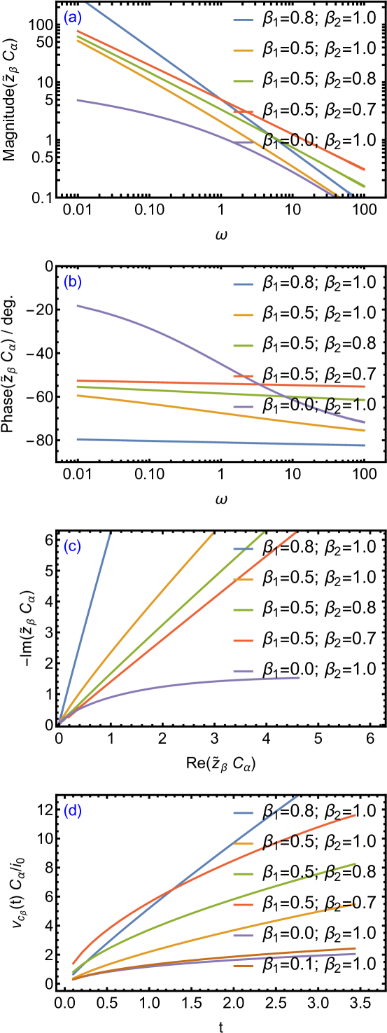
In Fig. 2 we show plots of the normalized impedance function $(z_{\beta}(s)\times C_{\alpha})$ in terms of its magnitude vs. frequency (see Fig. 2(a)), its phase vs. frequency (see Fig. 2(b)) and the real vs. imaginary parts (see Fig. 2(c)) for different combination values of $\beta_{1}$ and $\beta_{2}$. The case when $\beta_{1}=0$ and $\beta_{2}=1$, corresponding to the impedance given by Eq. 11, is also plotted in the figures and clearly represents the least capacitive network at low frequencies. For fixed $\beta_{2}=1$, the network becomes more capacitive as $\beta_{1}$ approaches one. We can also see from the figures that for the three cases where the upper limit $\beta_{2}$ is the same, i.e. ($\beta_{1}=0.8,\,\beta_{2}=1.0$), ($\beta_{1}=0.5,\,\beta_{2}=1.0$) and ($\beta_{1}=0.0,\,\beta_{2}=1.0$), the impedance phase tends to the same limit at high frequencies dictated by this value of $\beta_{2}$. Whereas when the lower limit $\beta_{1}$ is the same, i.e. ($\beta_{1}=0.5,\,\beta_{2}=1.0$), ($\beta_{1}=0.5,\,\beta_{2}=0.8$) and ($\beta_{1}=0.5,\,\beta_{2}=0.7$), the phase tends to the same limit at low frequencies. Otherwise, it is evident that with this particular superposition of CPEs ($\phi(\alpha)$ uniform distribution), the resulting system is not a CPE itself. The closest the impedance phase gets to a constant, and therefore to a traditional CPE, is when the limits of integration $\beta_{1}$ and $\beta_{2}$ are closer to each other as it is the case for ($\beta_{1}=0.8,\,\beta_{2}=1.0$) for example.

Now we derive the network’s voltage in response to a constant current excitation with $i(t)=i_{0}>0$ for $t>0$ (see Fig. 1), assuming that the network is initially uncharged. The developed voltage $v_{c_{u}}(t)$ on the network when $\beta_{1}=0$ and $\beta_{2}=1$ is given by:

	$\displaystyle v_{c_{u}}(t)$	$\displaystyle=\mathcal{L}^{-1}\left\{\frac{i_{0}}{C_{\alpha}}\frac{\ln(s)}{s(s-1)};t\right\}$		(16)
		$\displaystyle=\frac{i_{0}}{C_{\alpha}}\left[\gamma-e^{t}\text{Ei}(-t)+\ln(t)\right]$		(17)

where $\text{Ei}(z)=-\int_{-z}^{\infty}u^{-1}e^{-u}du$ is the exponential integral function and $\gamma$ is Euler’s constant $\approx 0.577216$. Similar results were reported by Eab and Lim [26] for the case of simple free fractional Langevin equation without a friction term.

The voltage expression for the general impedance function under the condition $0<\beta_{1}\leqslant\alpha\leqslant\beta_{2}<1$ can also be derived after applying the series expansion $(1-x)^{-1}=\sum_{k=0}^{\infty}x^{k}$ for $|x|<1$ enabling us to write:

	$\displaystyle v_{c_{\beta}}(t)$	$\displaystyle=\mathcal{L}^{-1}\left\{\frac{i_{0}}{C_{\alpha}}\frac{s^{-\beta_{2}-1}\ln(s)}{1-s^{\beta_{1}-\beta_{2}}};t\right\}$		(18)
		$\displaystyle=\frac{i_{0}}{C_{\alpha}}\mathcal{L}^{-1}\left\{\ln(s)\sum_{k=0}^{\infty}s^{-k(\beta_{2}-\beta_{1})-(\beta_{2}+1)};t\right\}$		(19)

Noting that the $\ln(s)$ function can be represented in terms of the Fox $H$-function as:

	$\displaystyle\ln(s)$	$\displaystyle=\ln(1+s)-\ln(1+s^{-1})$
		$\displaystyle=H^{1,2}_{2,2}\left[s\left|\begin{array}[]{l}(1,1),(1,1)\\ (1,1),(0,1)\\ \end{array}\right.\right]-H^{1,2}_{2,2}\left[s^{-1}\left|\begin{array}[]{l}(1,1),(1,1)\\ (1,1),(0,1)\\ \end{array}\right.\right]$		(24)

the inverse Laplace transform can then be evaluated term by term. Recall that the $H$-function of order $(m,n,p,q)\in\mathbb{N}^{4}$, ($0\leqslant n\leqslant p$, $1\leqslant m\leqslant q$) and with parameters $A_{j}\in\mathbb{R}_{+}\;(j=1,\ldots,p)$, $B_{j}\in\mathbb{R}_{+}\;(j=1,\ldots,q)$, $a_{j}\in\mathbb{C}\;(j=1,\ldots,p)$ and $b_{j}\in\mathbb{C}\;(j=1,\ldots,q)$ is defined for $z\in\mathbb{C},\;z\neq 0$ by the contour integral [18, 20]:

$$H^{m,n}_{p,q}\left[z\left|\begin{array}[]{c}{(a_{1},A_{1}),\ldots,(a_{p},A_{p})}\\ {(b_{1},B_{1}),\ldots,(b_{q},B_{q})}\end{array}\right.\right]=\frac{1}{2\pi i}\int_{L}h(s)z^{-s}ds$$

(25)

where the integrand $h(s)$ is given by:

$$h(s)=\frac{\left\{\prod\limits_{j=1}^{m}\Gamma(b_{j}+B_{j}s)\right\}\left\{\prod\limits_{j=1}^{n}\Gamma(1-a_{j}-A_{j}s)\right\}}{\left\{\prod\limits_{j={m+1}}^{q}\Gamma(1-b_{j}-B_{j}s)\right\}\left\{\prod\limits_{j={n+1}}^{p}\Gamma(a_{j}+A_{j}s)\right\}}$$

(26)

In Eq. 25, $z^{-s}=\exp\left[-s(\ln|z|+i\arg z)\right]$ and $\arg z$ is not necessarily the principal value. The contour of integration $L$ is a suitable contour separating the poles of $\Gamma(b_{j}+B_{j}s)$ ($j=1,\ldots,m$) from the poles of $\Gamma(1-a_{j}-A_{j}s)$ ($j=1,\ldots,n$). An empty product is always interpreted as unity. We also recall that the Laplace transform of an $H$-function which is given by [18]:

	$\displaystyle\mathcal{L}$	$\displaystyle\left[t^{\rho-1}H_{p,q}^{m,n}\left[at^{\sigma}\left|\begin{array}[]{l}(a_{p},A_{p})\\ (b_{q},B_{q})\\ \end{array}\right.\right];u\right]$		(29)
		$\displaystyle=u^{-\rho}H^{m,n+1}_{p+1,q}\left[au^{-\sigma}\left|\begin{array}[]{l}(1-\rho,\sigma),(a_{1},A_{1}),\ldots,(a_{p},A_{p})\\ (b_{1},B_{1}),\ldots,(b_{q},B_{q})\hfill\\ \end{array}\right.\right]$		(32)

and the inverse Laplace transform by [18]:

	$\displaystyle\mathcal{L}^{-1}$	$\displaystyle\left[u^{-\rho}H_{p,q}^{m,n}\left[au^{\sigma}\left|\begin{array}[]{l}(a_{p},A_{p})\\ (b_{q},B_{q})\\ \end{array}\right.\right];t\right]$		(35)
		$\displaystyle=t^{\rho-1}H_{p+1,q}^{m,n}\left[at^{-\sigma}\left|\begin{array}[]{l}(a_{p},A_{p}),\ldots,(a_{1},A_{1}),(\rho,\sigma)\\ (b_{1},B_{1}),\ldots,(b_{q},B_{q})\hfill\end{array}\right.\right]$		(38)

Thus we obtain the general solution for $v_{c_{\beta}}(t)$ given by Eq. 19 as:

	$\displaystyle v_{c_{\beta}}(t)=\frac{i_{0}}{C_{\alpha}}\sum_{k=0}^{\infty}t^{\rho_{k}-1}$	$\displaystyle\left\{H^{1,2}_{3,2}\left[t^{-1}\left|\begin{array}[]{l}(1,1),(1,1),({\rho_{k}},1)\\ (1,1),(0,1)\end{array}\right.\right]\right.$		(41)
		$\displaystyle\left.-H^{1,2}_{3,2}\left[t\left|\begin{array}[]{l}(1,1),(1,1),({\rho_{k}},-1)\\ (1,1),(0,1)\end{array}\right.\right]\right\},$		(44)

where $\rho_{k}=k(\beta_{2}-\beta_{1})+(\beta_{2}+1)$. This represents the total voltage developed across the network with the only constraint being that $0<\beta_{1}\leqslant\alpha\leqslant\beta_{2}<1$.

In Fig. 2(d) we plot the normalized network voltage $(v_{c_{\beta}}(t)\times C_{\alpha}/i_{0})$ as given by Eq. 44 for different values of $\beta_{1}$ and $\beta_{2}$. The summation was truncated to the first 40 terms. Also, the normalized network voltage $(v_{c_{u}}(t)\times C_{\alpha}/i_{0})$ given by Eq. 17 (i.e. when $\beta_{1}=0.0$ and $\beta_{1}=1.0$) is plotted in the same figure. Correspondingly, a plot is shown for the case of $\beta_{1}=0.1,\,\beta_{2}=1.0$ in order to compare the accuracy of plotting the $H$-function based expression vs. directly plotting Eq. 17 (valid only for $\beta_{1}=0.0,\,\beta_{2}=1.0$). It can be clearly seen that in both these cases, the steady-state normalized voltage (i.e. at $t\rightarrow\infty$) has the lowest value because the network is least capacitive, as expected. The higher the value of the steady-state voltage, the more capacitive the network is. In particular, at a first glance when comparing the voltage profiles simulated with ($\beta_{1}=0.8,\,\beta_{2}=1.0$), ($\beta_{1}=0.5,\,\beta_{2}=1.0$) and ($\beta_{1}=0.0,\,\beta_{2}=1.0$) having the same values for $\beta_{2}$, it appears that the more the interval $[\beta_{1},\beta_{2}]$ is skewed to one, the higher is the magnitude of the voltage. But for ($\beta_{1}=0.5,\,\beta_{2}=1.0$), ($\beta_{1}=0.5,\,\beta_{2}=0.8$) and ($\beta_{1}=0.5,\,\beta_{2}=0.7$), which are all having the same lower limit $\beta_{1}$, the voltage magnitude seems to be higher as the value of $\beta_{2}$ approaches that of $\beta_{1}$. The same remark now holds for fixed value of $\beta_{2}$ just discussed previously. But if we compare the two cases of ($\beta_{1}=0.8,\,\beta_{2}=1.0$) and ($\beta_{1}=0.5,\,\beta_{2}=0.7$), wherein the size of the interval for $\alpha$ is 0.2 for both, we can clearly see a crossing point below which the latter case generate higher voltage, and vice versa, i.e. above this crossing point it is the voltage corresponding to ($\beta_{1}=0.8,\,\beta_{2}=1.0$) that overtakes the other. This is an interesting observation that highlights the difference in response time of distributed order CPEs at small vs. larger values of time.

As a second example, we consider the case where the weight function for the order $\alpha$ is given by:

$$\phi(\alpha)=\sum_{i}C_{\alpha_{i}}\,\delta(\alpha-\alpha_{i})$$

(45)

with $\delta(x)$ the Dirac delta function.

The network’s equivalent impedance is straightforward to obtain in this case. For example, for $i=2$, the network contains only two CPEs with different parameters, and its equivalent impedance is simply:

$\displaystyle\tilde{z}_{2}(s)$

$\displaystyle=\frac{1}{C_{\alpha_{1}}s^{\alpha_{1}}+C_{\alpha_{2}}s^{\alpha_{2}}}$

(46)

This means that we have a total current in the system being:

$$i_{2}(t)=C_{\alpha_{1}}\,{}_{0}\text{D}_{t}^{\alpha_{1}}v_{c}(t)+C_{\alpha_{2}}\,{}_{0}\text{D}_{t}^{\alpha_{2}}v_{c}(t)$$

(47)

and therefore the order distribution function $\phi(\alpha)$ is:

$$\phi_{2}(\alpha)=C_{\alpha_{1}}\,\delta(\alpha-\alpha_{1})+C_{\alpha_{2}}\,\delta(\alpha-\alpha_{2})$$

(48)

While for $i=3$, i.e. the case of three CPEs in parallel the equivalent impedance is:

$\displaystyle\tilde{z}_{3}(s)=\frac{1}{C_{\alpha_{1}}s^{\alpha_{1}}+C_{\alpha_{2}}s^{\alpha_{2}}+C_{\alpha_{3}}s^{\alpha_{3}}}$

(49)

and for the general case, the total network input admittance is the sum:

$\displaystyle\tilde{y}_{i}(s)$

$\displaystyle={C_{\alpha_{1}}s^{\alpha_{1}}+C_{\alpha_{2}}s^{\alpha_{2}}}+.....+C_{\alpha_{i}}s^{\alpha_{i}}$

(50)

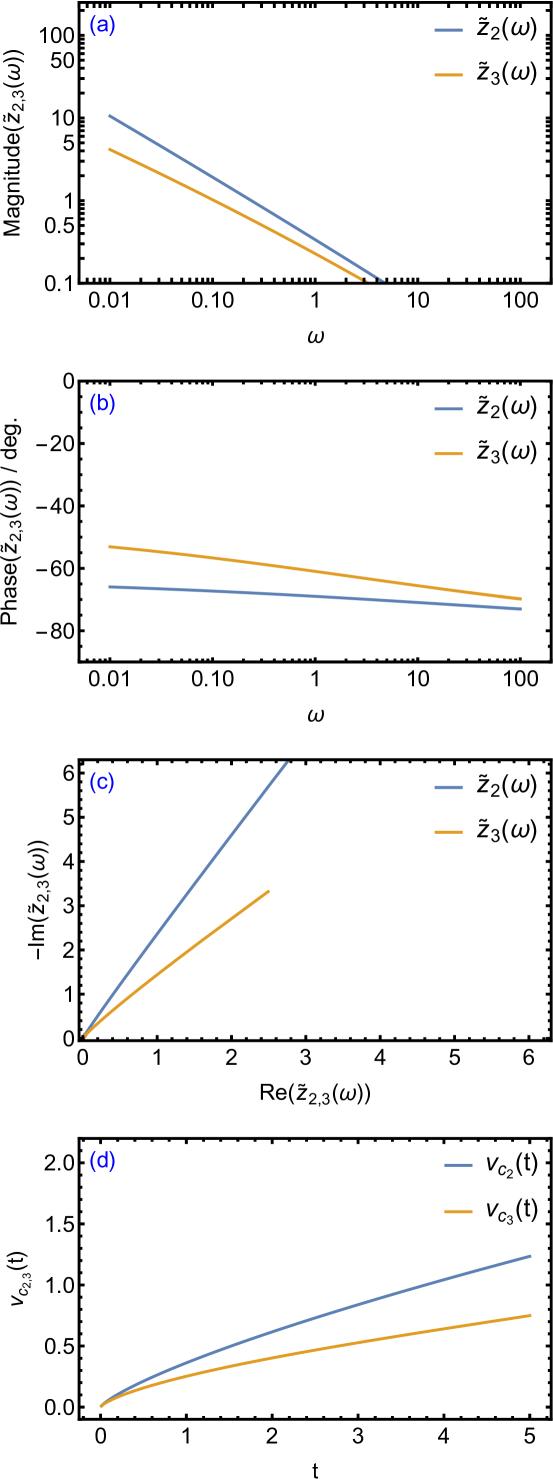
For illustration purposes, we show in Fig. 3 plots of $\tilde{z}_{2}(s)$ (Eq. 46) and $\tilde{z}_{3}(s)$ (Eq. 49) in terms of magnitude vs. frequency (Fig. 3(a)), phase vs. frequency (Fig. 3(b)) and real vs. imaginary parts (Fig. 3(c)) with the parameters values ($\alpha_{1}=0.9$, $C_{\alpha_{1}}=1.0\,\text{F\,s}^{\alpha_{1}-1}$), ($\alpha_{2}=0.9$, $C_{\alpha_{2}}=2.0\,\text{F\,s}^{\alpha_{2}-1}$), ($\alpha_{3}=0.5$, $C_{\alpha_{3}}=1.5\,\text{F\,s}^{\alpha_{3}-1}$), over the frequency range 0.01 to 100 Hz. The effect of adding the third less-capacitive CPE (with $\alpha=0.5$) on the overall network impedance is clear from the figures.

Deriving in closed form the expression for the voltage response across the network is done here after recalling the Laplace transform formula [29, 30]:

$$\int\limits_{0}^{\infty}t^{\beta-1}{E}_{\alpha,\beta}^{\gamma}\left(-at^{\alpha}\right)e^{-st}dt=\frac{s^{-\beta}}{(1+as^{-\alpha})^{\gamma}}$$

(51)

where

$$\text{E}_{\alpha,\beta}^{\gamma}(z):=\sum\limits_{k=0}^{\infty}\frac{(\gamma)_{k}}{\Gamma(\alpha k+\beta)}\frac{z^{k}}{k!}\quad(\alpha,\beta,\gamma\in\mathbb{C},\mathrm{Re}({\alpha})>0)$$

(52)

is the generalized Mittag-Leffler function [29] and $(\gamma)_{k}=\Gamma(\gamma+k)/\Gamma(\gamma)$ is the Pochhammer symbol. We can obtain directly the time-domain voltage in response to a constant current excitation $i(t)=i_{0}>0$ for $t>0$ applied on the (initially uncharged) network with two CPEs only as:

$$v_{c_{2}}(t)=C_{\alpha_{1}}^{-1}{i_{0}}\,t^{\alpha_{1}}\text{E}_{\alpha_{1}-\alpha_{2},\alpha_{1}+1}(-C_{\alpha_{1}}^{-1}C_{\alpha_{2}}t^{\alpha_{1}-\alpha_{2}})$$

(53)

Note that the Mittag-Leffler function can also be expressed as an $H$-function [18] in the form:

$$\text{E}_{\alpha,\beta}^{\gamma}(z)=\frac{1}{\Gamma(\gamma)}H^{1,1}_{1,2}\left[-z\left|\begin{array}[]{l}(1-\gamma,1)\\ (0,1),(1-\beta,\alpha)\\ \end{array}\right.\right]$$

(54)

We verify that when $\alpha_{1}=\alpha_{2}$ in Eq. 53, the voltage simplifies to:

$$v_{c_{2}}(t)=\frac{{i_{0}}\,t^{\alpha_{1}}}{(C_{\alpha_{1}}+C_{\alpha_{2}})\Gamma(1+\alpha_{1})}$$

(55)

and if we additionally have $C_{\alpha_{1}}=C_{\alpha_{2}}$, then

$$v_{c_{2}}(t)=\frac{{i_{0}}\,t^{\alpha_{1}}}{2C_{\alpha_{1}}\Gamma(1+\alpha_{1})}$$

(56)

as expected.

Now for the case of three CPEs in the network and under the assumption that $\alpha_{1}>\alpha_{2}>\alpha_{3}$, it can be shown that the network equivalent impedance given by Eq. 49 can be rewritten as:

	$\displaystyle\tilde{z}_{3}(s)$	$\displaystyle=\cfrac{C_{\alpha_{1}}^{-1}s^{-\alpha_{1}}}{1+C_{\alpha_{1}}^{-1}C_{\alpha_{2}}s^{\alpha_{2}-\alpha_{1}}}\cfrac{1}{1+\cfrac{C_{\alpha_{1}}^{-1}C_{\alpha_{3}}s^{\alpha_{3}-\alpha_{1}}}{1+C_{\alpha_{1}}^{-1}C_{\alpha_{2}}s^{\alpha_{2}-\alpha_{1}}}}$		(57)
		$\displaystyle=C_{\alpha_{1}}^{-1}\sum\limits_{k=0}^{\infty}\left(-C_{\alpha_{1}}^{-1}C_{\alpha_{3}}\right)^{k}\cfrac{s^{-\alpha_{1}+k(\alpha_{3}-\alpha_{1})}}{\left(1+C_{\alpha_{1}}^{-1}C_{\alpha_{2}}s^{\alpha_{2}-\alpha_{1}}\right)^{k+1}}$		(58)

with the use of the expansion formula $(1+x)^{-1}=\sum_{k=0}^{\infty}(-1)^{k}x^{k}$ for $|x|<1$. Its inverse Laplace transform is carried out term by term using Eq. 51 leading to:

	$\displaystyle z_{3}(t)=C_{\alpha_{1}}^{-1}t^{\alpha_{1}-1}\sum\limits_{k=0}^{\infty}$	$\displaystyle\left(-C_{\alpha_{1}}^{-1}C_{\alpha_{3}}\right)^{k}t^{{-k(\alpha_{3}-\alpha_{1})}}$
		$\displaystyle\times\text{E}_{\alpha_{1}-\alpha_{2},{\alpha_{1}-k(\alpha_{3}-\alpha_{1})}}^{k+1}\left(-C_{\alpha_{1}}^{-1}C_{\alpha_{2}}t^{\alpha_{1}-\alpha_{2}}\right)$		(59)

Under a constant current excitation, the resulting voltage for this case is found to be:

	$\displaystyle v_{c_{3}}(t)=i_{0}C_{\alpha_{1}}^{-1}t^{\alpha_{1}}\sum\limits_{k=0}^{\infty}$	$\displaystyle\left(-C_{\alpha_{1}}^{-1}C_{\alpha_{3}}\right)^{k}t^{{-k(\alpha_{3}-\alpha_{1})}}$
		$\displaystyle\times\text{E}_{\alpha_{1}-\alpha_{2},{\alpha_{1}+1-k(\alpha_{3}-\alpha_{1})}}^{k+1}\left(-C_{\alpha_{1}}^{-1}C_{\alpha_{2}}t^{\alpha_{1}-\alpha_{2}}\right)$		(60)

The solution to a similar problem for $n$ discrete terms as depicted in Fig. 1, i.e. for a total current of the form:

$$i_{n}(t)=C_{\alpha_{1}}\,{}_{0}\text{D}_{t}^{\alpha_{1}}v_{c}(t)+C_{\alpha_{2}}\,{}_{0}\text{D}_{t}^{\alpha_{2}}v_{c}(t)+\ldots+C_{\alpha_{n}}\,{}_{0}\text{D}_{t}^{\alpha_{n}}v_{c}(t)$$

(61)

and thus a weight function,

$$\phi_{n}(\alpha)=C_{\alpha_{1}}\,\delta(\alpha-a_{1})+C_{\alpha_{2}}\,\delta(\alpha-a_{2})+\ldots+C_{\alpha_{n}}\,\delta(\alpha-a_{n})$$

(62)

can be found in Podlubny [31].

In Fig. 3(d), we plotted the time-domain voltage expressions given by Eq. 53 and by Eq. 60 (first 10 terms of the sum) using the same parameter values, and with $i_{0}=1$. The voltage growth follows non-exponential, power-law like profiles which is expected [8, 22, 32]. The effect of the less capacitive CPE (with $\alpha=0.5$) on reducing the steady-state value of the voltage is clear from the figure. Similar results can be obtained for more than three CPEs in the network.

References

- [1] J. A. Amani, T. Koppe, H. Hofsaess, U. Vetter, Analysis of immittance spectra: Finding unambiguous electrical equivalent circuits to represent the underlying physics, Phys. Rev. Appl. 4 (4) (2015) 044007.
- [2] J.-B. Jorcin, M. E. Orazem, N. Pébère, B. Tribollet, Cpe analysis by local electrochemical impedance spectroscopy, Electrochim. Acta 51 (8-9) (2006) 1473–1479.
- [3] S. M. Gateman, O. Gharbi, H. G. de Melo, K. Ngo, M. Turmine, V. Vivier, On the use of a constant phase element (cpe) in electrochemistry, Curr. Opin. Electrochem. 36 (2022) 101133.
- [4] M. E. Orazem, I. Frateur, B. Tribollet, V. Vivier, S. Marcelin, N. Pébère, A. L. Bunge, E. A. White, D. P. Riemer, M. Musiani, Dielectric properties of materials showing constant-phase-element (cpe) impedance response, J. Electrochem. Soc. 160 (6) (2013) C215.
- [5] X. Vendrell, J. Ramírez-González, Z.-G. Ye, A. R. West, Revealing the role of the constant phase element in relaxor ferroelectrics, Commun. Phys. 5 (1) (2022) 9.
- [6] M. S. Abouzari, F. Berkemeier, G. Schmitz, D. Wilmer, On the physical interpretation of constant phase elements, Solid State Ionics 180 (14-16) (2009) 922–927.
- [7] A. Allagui, A. Elwakil, E. H. Balaguera, Exact solution for the electrical response of a constant phase element with a series resistance to linear voltage sweep, J. Power Sources 613 (2024) 234907.
- [8] A. Allagui, H. Benaoum, Power-law charge relaxation of inhomogeneous porous capacitive electrodes, J. Electrochem. Soc. 169 (2022) 040509.
- [9] A. Allagui, M. E. Fouda, Inverse problem of reconstructing the capacitance of electric double-layer capacitors, Electrochim. Acta (2021) 138848.
- [10] A. Allagui, M. Fouda, A. S. Elwakil, The ragone plot of supercapacitors under different loading conditions, J. Electrochem. Soc. 167 (2) (2020) 020533.
- [11] A. Lasia, The origin of the constant phase element, The Journal of Physical Chemistry Letters 13 (2) (2022) 580–589.
- [12] M. Caputo, Distributed order differential equations modelling dielectric induction and diffusion, Fract. Calc. Appl. Anal. 4 (4) (2001) 421–442.
- [13] W. Ding, S. Patnaik, S. Sidhardh, F. Semperlotti, Applications of distributed-order fractional operators: A review, Entropy 23 (1) (2021) 110.
- [14] S. Patnaik, J. P. Hollkamp, F. Semperlotti, Applications of variable-order fractional operators: a review, Proc. R. Soc. A 476 (2234) (2020) 20190498.
- [15] R. Bagley, P. Torvik, On the existence of the order domain and the solution of distributed order equations-part i, Int. J. Appl. Math. 2 (7) (2000) 865–882.
- [16] R. Bagley, P. Torvik, On the existence of the order domain and the solution of distributed order equations-part ii, Int. J. Appl. Math. 2 (8) (2000) 965–988.
- [17] H. J. Haubold, A. M. Mathai, R. K. Saxena, Mittag-leffler functions and their applications, J. Appl. Math. 2011.
- [18] A. M. Mathai, R. K. Saxena, H. J. Haubold, The H-function: theory and applications, Springer Science & Business Media, 2009.
- [19] A. Mathai, H. J. Haubold, Mittag-leffler functions and fractional calculus, Special Functions for Applied Scientists (2008) 79–134.
- [20] A. M. Mathai, R. K. Saxena, R. K. Saxena, et al., The H-function with applications in statistics and other disciplines, John Wiley & Sons, 1978.
- [21] A. Allagui, E. H. Balaguera, On the semi-infinite distributed resistor-constant phase element transmission line, Electrochim. Acta 510 (2025) 145344.
- [22] A. Allagui, A. S. Elwakil, Possibility of information encoding/decoding using the memory effect in fractional-order capacitive devices, Sci. Rep. 11 (1) (2021) 1–7.
- [23] A. Allagui, A. S. Elwakil, C. Psychalinos, Decoupling the magnitude and phase in a constant phase element, J. Electroanal. Chem. 888 (2021) 115153.
- [24] A. Allagui, A. S. Elwakil, Tikhonov regularization for the deconvolution of capacitance from voltage-charge response of electrochemical capacitors, Electrochim. Acta (2023) 142527.
- [25] C. F. Lorenzo, T. T. Hartley, Variable order and distributed order fractional operators, Nonlinear Dyn. 29 (2002) 57–98.
- [26] C. Eab, S. Lim, Fractional langevin equations of distributed order, Phys. Rev. E 83 (3) (2011) 031136.
- [27] F. Mainardi, A. Mura, G. Pagnini, R. Gorenflo, Time-fractional diffusion of distributed order, J. Vib. Control 14 (9-10) (2008) 1267–1290.
- [28] Z. Said, A. Allagui, M. A. Abdelkareem, A. S. Elwakil, H. Alawadhi, R. Zannerni, K. Elsaid, Modulating the energy storage of supercapacitors by mixing close-to-ideal and far-from-ideal capacitive carbon nanofibers, Electrochim. Acta 301 (2019) 465–471.
- [29] T. R. Prabhakar, A singular integral equation with a generalized Mittag Leffler function in the kernel, Yokohama Math. J. 19 (1) (1971) 7–15.
- [30] R. Saxena, A. Mathai, H. Haubold, On generalized fractional kinetic equations, Physica A 344 (3-4) (2004) 657–664.
- [31] I. Podlubny, Fractional differential equations: an introduction to fractional derivatives, fractional differential equations, to methods of their solution and some of their applications, Elsevier, 1998.
- [32] A. Allagui, H. Benaoum, A. S. Elwakil, M. Alshabi, Extended impedance and relaxation models for dissipative electrochemical capacitors, IEEE Trans. Electron Devices (2022).