On The Calibration of Short-Term Interest Rates Through a CIR Model
Abstract
It is well known that the Cox-Ingersoll-Ross (CIR) stochastic model to study the term structure of interest rates, as introduced in 1985, is inadequate for modelling the current market environment with negative short interest rates. Moreover, the diffusion term in the rate dynamics goes to zero when short rates are small; both volatility and long-run mean do not change with time; they do not fit with the skewed (fat tails) distribution of the interest rates, etc. The aim of the present work is to suggest a new framework, which we call the CIR# model, that well fits the term structure of short interest rates so that the market volatility structure is preserved as well as the analytical tractability of the original CIR model.
keywords:
Interest rates forecasting, volatility, ARIMA models, simulation, jumps fitting, translationJEL Classification: G12, E43, E47
MSC:
[2010] 91G30, 91B84, 91G60, 91G70, 62M101 Introduction
The aim of the present work is to provide a new numerical methodology for the CIR framework, which we call the CIR# model, that well fits the term structure of short interest rates as observed in a real market. Our approach is based on a proper translation of interest rates so that the market volatility structure is preserved as well as the analytical tractability of the original CIR model.
Cox, Ingersoll & Ross (1985) [11] proposed a term structure model, well known as the CIR model, to describe the price of discount zero-coupon bonds with variuous maturities under no-arbitrage condition. This model generalizes the Vasicek model [34] to the case of non constant volatility and assumes that the evolution of the underlying short term interest rate is a diffusion process, i.e. a continuous Markov process unique solution to the following stochastic differential equation (SDE)
| (1) |
with initial condition . denotes a standard Brownian motion under the risk neutral probability measure, intended to model a random risk factor. The interest rate process is usually known as the CIR process or square root process. The SDE (1) is classified as a one-factor time-homogeneous model, because the parameters and are time-independent and the short interest rate dynamic is driven only by the market price of risk where is a constant. Therefore the SDE (1) is composed of two parts: the “mean reverting” drift component which ensures the rate is elastically pulled towards a long-run mean value at a speed of adjustment and the random component which is scaled by the standard deviation . The volatility of the instantaneous short rate is denoted by .
The paths of the CIR process never reach negative values and their behaviour depends on the relationship between the three constant positive parameters . Indeed, it can be shown (see, e.g., Jeanblanc, Yor & Chesney (2009) [19, Ch. 3]) that if the condition is satisfied, then the interest rates are strictly positive for all , and, for small , the process rebounds as the random perturbation dampens with . Furthermore, the CIR process belongs to the class of processes satisfying the “affine property”, i.e., the logarithm of the characteristic function of the transition distribution of such processes is an affine (linear plus constant) function with respect to their initial state (for more details the reader can refer to Duffie, Filipović & Schachermayer (2003) [13, Section 2]. As a consequence, the non-arbitrage price of a discount zero coupon bond with maturity and underlying interest rate dynamics described by a CIR process, is given by
| (2) |
where and are deterministic functions (see Cox, Ingersoll & Ross (1985) [11]). The final condition is which corresponds to the nominal value of the bond conventionally set equal to 1 (monetary unit). Since bonds are commonly quoted in terms of yields rather than prices, the formula (2) allows derivation of the yield-to-maturity curve
which tends to the asymptotic value as where
Thus the CIR process is characterized by the following properties: 1) short interest rates never become negative; 2) if the interest rate reaches the zero value (it may occur under the condition ), it is immediately reflected in positive values; 3) the diffusion term in (1) increases when increases; 4) the transition density of short rates is a noncentral chi-squared distribution, which converges to a gamma distribution as time grows towards infinity; 5) the trajectories describing the short rate dynamics cannot be explicitly derived, but exact simulation is still possible and bond prices are explicitly computable from it.
The remainder of the paper is organized as follows. Section 2 summarizes the existing literature on the CIR model and the related extensions. Section 3 describes the principal steps of the proposed CIR# model; Section 4 presents in more detail the numerical procedure and tests the goodness-of-fit of the new methodology to market data. Finally, Section 5 concludes.
2 Literature review
The CIR model became very popular in finance among practitioners because it was perceived as an improvement on the Vasicek model, not allowing for negative rates and introducing a rate dependent volatility, as well as for its relatively handy implementation and analytical tractability. Other applications include stochastic volatility modelling in option pricing problems (see Orlando and Taglialatela (2017) [32], Heston (1993) [16]), or default intensities in credit risk (see Duffie (2005) [12]).
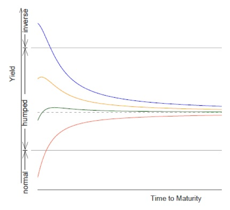
Despite the previously listed properties, the CIR model fails as a satisfactory calibration to market data since it depends on a small number of constant parameters, and As proved by Keller-Ressel and Steiner (2008) [22, Theorem 3.9 and Section 4.2] the yield-to-maturity curve of any time-homogenous, affine one-factor model is either normal (i.e., a strictly increasing function of ), humped (i.e., with one local maximum and no minimum on ) or inverse (i.e., a strictly decreasing function of ) (see Figure 1). For the CIR process, the yield is normal when , while it is inverse when For intermediate values the yield curve is humped.
However, Carmona and Tehranchi (2006), [9, Section 2.3.5] explained that: “Tweaking the parameters can produce yield curves with one hump or one dip (a local minimum), but it is very difficult (if not impossible) to calibrate the parameters so that the hump/dip sits where desired. There are not enough parameters to calibrate the models to account for observed features contained in the prices quoted on the markets” (see Figure 2).
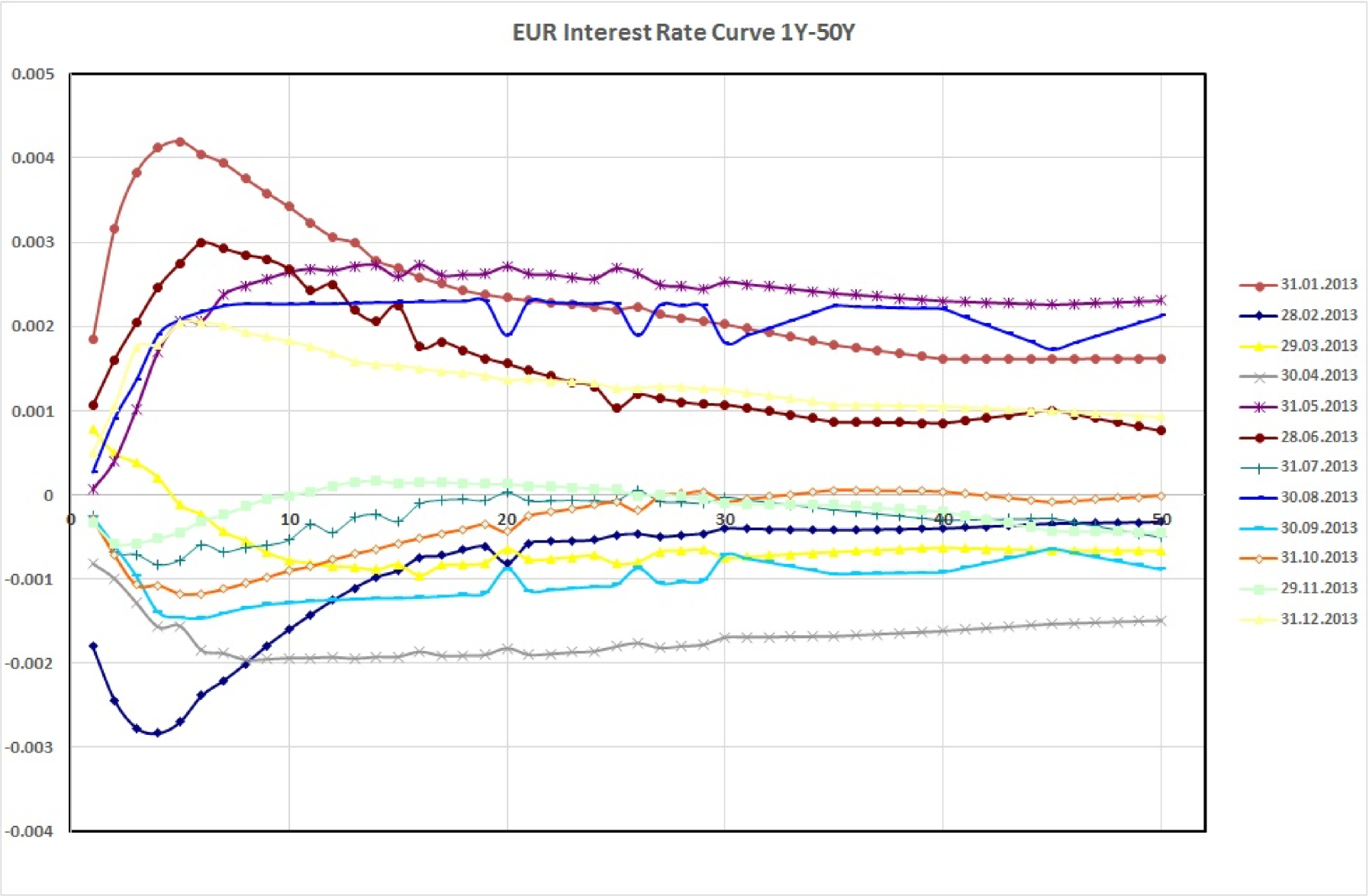
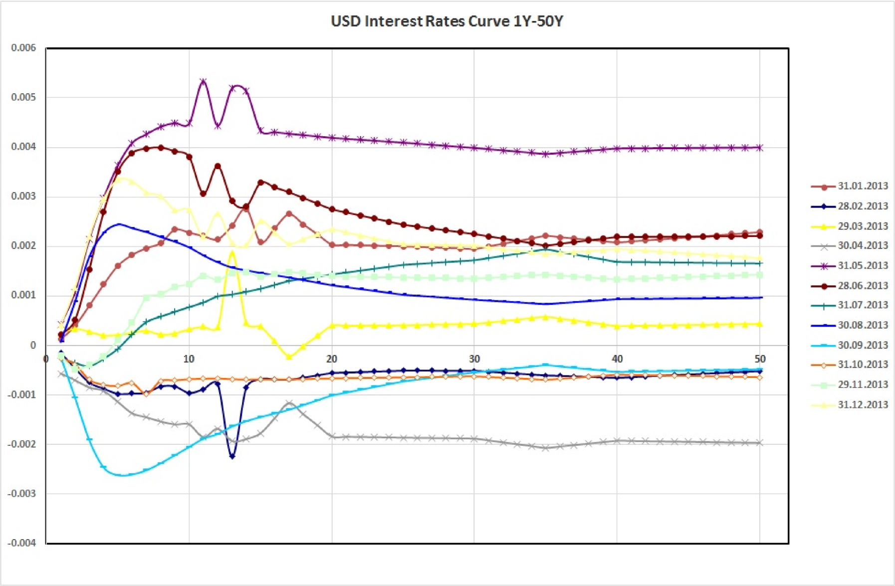
Thus the need for more sophisticated models for an exact fit to the currently-observed yield curve, which could take into account multiple correlated sources of risk as well as shocks and/or structural changes of the market, led some years later to the development of extensions of the CIR model. Among the best known we mention: the Hull-White (1990) [17] model based on the idea of considering time-dependent coefficients; the Chen (1996) [10] three-factor model; the CIR++ model by Brigo & Mercurio (2001) [7] that considers short rates shifted by a deterministic function chosen to fit exactly the initial term structure of interest rates; the jump diffusion JCIR model (see Brigo & Mercurio (2006) [8]) and JCIR++ by Brigo & El-Bachir (2006)[6] where jumps are described by a time-homogeneous Poisson process; the CIR2 and CIR2++ two-factor models (see Brigo & Mercurio (2006) [8]). Very recently, Zhu (2014) [35], in order to incorporate the default clustering effects, proposed a CIR process with jumps modelled by a Hawkes process (which is a point process that has self-exciting property and the desired clustering effect), Moreno et al. (2015) [27] presented a cyclical square-root model, and Najafi et al. (2017) ([28], [29]) proposed some extensions of the CIR model where a mixed fractional Brownian motion applies to display the random part of the model.
Note that all the above cited extensions to CIR model preserve the positivity of interest rates, in some cases through reasonable restrictions on the parameters. But the financial crisis of 2008 and the ensuing quantitative easing policies brought down interest rates, as a consequence of reduced growth of developed economies, and accustomed markets to unprecedented negative interest regimes under the so called “new normal”. As observed in Engelen (2015) [14] and BIS (2015) [5]:
“Interest rates have been extraordinarily low for an exceptionally long time, in nominal and inflation-adjusted terms, against any benchmark”(see Figure 3). “Between December 2014 and end-May 2015, on average around $2 trillion in global long-term sovereign debt, much of it issued by euro area sovereigns, was trading at negative yields”, “such yields are unprecedented. Policy rates are even lower than at the peak of the Great Financial Crisis in both nominal and real terms. And in real terms they have now been negative for even longer than during the Great Inflation of the 1970s. Yet, exceptional as this situation may be, many expect it to continue”. ”Such low rates are the most remarkable symptom of a broader malaise in the global economy: the economic expansion is unbalanced, debt burdens and financial risks are still too high, productivity growth too low, and the room for manoeuvre in macroeconomic policy too limited. The unthinkable risks becoming routine and being perceived as the new normal.”
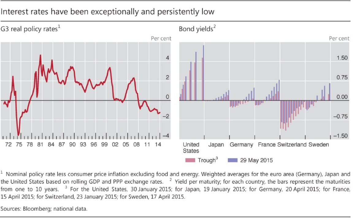
Therefore, the need for adjusting short term interest rate models for negative rates has become an additional characteristic that a “good” model should possess. It is worth noting that the main drawback of the Vasicek model [34], which allows for negative interest rates, is that the conditional volatility of changes in the interest rate is constant, independent on the level of it, and this may unrealistically affect the prices of bonds that can grow exponentially (see Rogers [33]). For this reason, the Vasicek model is unused by practitioners.
3 The CIR# model
In the following we will illustrate our original approach, but first let us recap the main issues of the CIR model:
-
i.
Negative interest rates are precluded;
-
ii.
The diffusion term in (1) goes to zero when is small (in contrast with market data);
-
iii.
The instantaneous volatility is constant (in real life is calibrated continuously from market data);
-
iv.
There are no jumps (e.g. caused by government fiscal and monetary policies, by release of corporate financial results, etc.);
-
v.
Risk premia are linear with interest rates (false if credit worthiness of a counterparty and market volatility are considered);
-
vi.
The change in interest rates depends only on the market risk.
The aim of the present work is to provide a new methodology that gives an answer to points i.- iv. by preserving the structure of the original CIR model (1) to describe the dynamics of spot interest rates observed in financial markets. For this purpose the first step is partitioning the available market data sample into sub-samples - not necessarily of the same size - in order to capture all the statistically significant changes of variance in real spot rates and consequently, to give an account of jumps (see Section 4.2). This should allow to overcome the critical issue pointed out in iv.. After that, to overcome challenges i.- ii., the real spot rates are properly translated to shift them away from zero or negative values and such that the diffusion term in (1) is not dampened by the proximity to zero but fully reflects the same level of volatility present on the market (see Section 4.3).
The second step consists in fitting an “optimal” - as explained in Section 4.5 - ARIMA model to each sub-sample of market data. To ensure that the residuals of the chosen “optimal” ARIMA model in each sub-sample look like Gaussian white noise, the Johnson’s transformation (Johnson (1949)[20]) is applied to the standardized residuals (see Section 4.4).
As a third step, the parameters in (1) are calibrated to the (eventually) shifted market interest rates by estimating them for each sub-sample of available data, as explained in Section 4.4.1 (which allows to overcome the issue iii.). For this purpose, trajectories of the CIR process are simulated by a strong convergent discretization scheme, using the standardized residuals of the “optimal” ARIMA model selected for each sub-sample in place of realizations of a standard Brownian motion. As a result, exact CIR fitted values to real data are calculated and the computational cost of the numerical procedure is considerably reduced. Finally, the short-term interest rates estimated by the CIR model are shifted back and compared to real data. As a measure of goodness-of-fit to the available market data, we compute:
-
1.
the statistics given by the following expression [23]
(3) where denotes the residual between the observed market interest rate and the corresponding fitted value evaluated on a data sample of size Furthermore, and denote the sample mean of and , respectively;
-
2.
the square root of the mean square error (RMSE)
(4)
4 Numerical Implementation and Empirical Analysis
4.1 The Dataset
In this section we give explicit numerical results for the CIR# model described in Section 3. Our dataset records EUR and USD interest rates with maturities 1/360A–360/360A and 1Y–50Y (i.e. at 1 day (overnight), 30 days, 60 days,…., 360 days and 1 Year,…,50 Years) available from IBA [18]. For each maturity, interest rates are recorded on monthly basis from 31 December 2010 to 29 July 2016 for a total number of 68 datapoints. In the book [30](2018) we performed a qualitative analysis on this dataset. We found that the most challenging task was to fit short-term interest rates with maturity 1/360A, 30/360A, 60/360A, 90/360A, 120/360A,…, 360/360A, respectively, due to the presence of next-to-zero and/or negative spot rate values. This led us to implement a novel numerical procedure, the CIR model, that would allow description of the short-term structure by the original CIR model. The new methodology will be discussed in more details in the next subsections and we will give explicit numerical results for the CIR model applied to the data sample consisted of EUR interest rates with 1 day (overnight) maturity. All computations have been executed using MATLAB® Ra.
4.2 ANOVA test with a fixed segmentation
As explained in Section 3, our first objective is to overcome the issues pointed out in i., ii. and iv. for the CIR model. Thus we start to partition the whole data sample into sub-samples, which we call groups, by a one-way ANOVA analysis to highlight statistically significant changes of variance in real spot rates and so to give an account of possible jumps. The main difficulty concerns the choice of the optimal partition into groups to apply the ANOVA test; we had to take into account both the size (the smaller the group is, the more refined the analysis) and the ability to capture any jumps (the larger the group, the better in terms of statistical significance).
After several tests, we decided to segment the whole sample into eight groups each of size or a multiple thereof (except for the last group, obviously). The results of the one-way ANOVA test are reported in Table 1. The p-value (ProbF) of indicates a statistically significant difference between groups.
| Source | SS | df | MS | F | ProbF |
|---|---|---|---|---|---|
| Groups | 10.8783 | 7 | 1.55405 | 34.71 | 8.00796e-19 |
| Error | 2.6862 | 60 | 0.04477 | ||
| Total | 13.5645 | 67 |
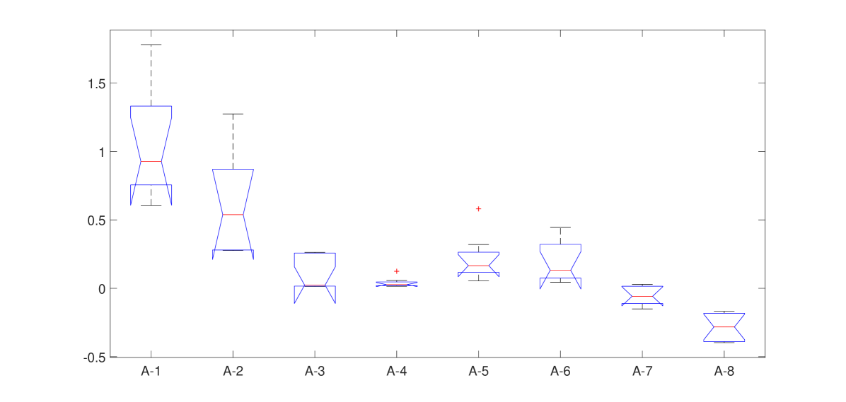
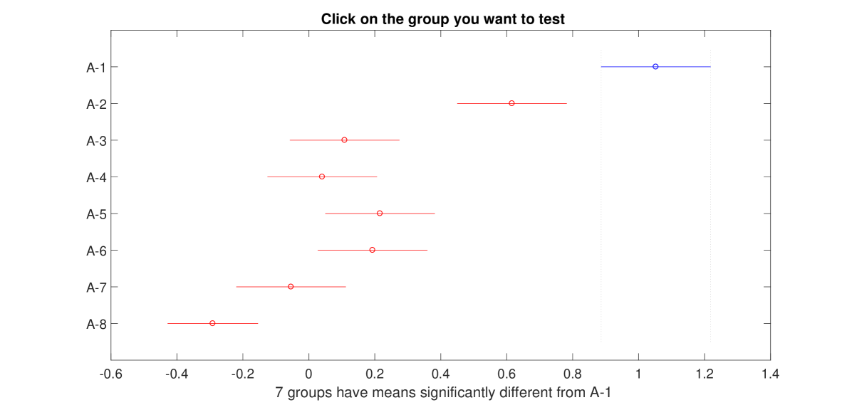
Furthermore, the boxplot (Figure 4.a)) and a multiple comparison test performed on the eight groups (Figure 4.b)) have suggested partitioning the data sample into the following four groups of observations 1–8, 9–16, 17–56, 57–68.
a)
b)
4.3 Jumps fitting by translation
Since the CIR model (1) does not fit negative interest rates and normal/high volatility when the rate value is small, spot rates must be shifted away from zero and/or negative values.
One chance is given by an affine type transformation, as follows
where and are the sample mean and the sample standard deviation of respectively. But, in practice, this is not the best choice due to some potential issues such as persistence of negative values, worse fitting, changes in the short interest rates behaviour, etc. Among different options, a translation of type
| (5) |
with a constant term, is a reasonable choice because it leaves unchanged the stochastic dynamics of short interest rates, i.e. . The value of the parameter can be arbitrarily selected but, in our opinion, the most appropriate choice must take into account the empirical distribution of interest rates. For our purpose, we set equal to the approximate value, calculated from the available market data, corresponding to the -percentile of the conditional distribution of the process However, if further negative values are between the - and the -percentile, then can be set equal to the approximate value corresponding to the -percentile of the conditional distribution of spot rates. Hence the translation (5) becomes .
The translation is applied after a check carried out on each group partitioning the original data sample; the check consists in calculating the harmonic mean - because it is more robust than the arithmetic one in the presence of extreme values - and in verifying whether it is smaller than a constant value arbitrarily chosen small (e.g. ). If this happens in at least one group, then the whole sample is translated.
4.4 Sub-optimal ARIMA models
The second step consists in deriving the best fitting ARIMA model to each group of interest rates partitioning the original market data sample. Thus we start by selecting, for each group, a set of ARIMA models whose standardized residuals satisfy the following “sub-optimal” conditions:
-
1.
Absence of both autocorrelation (AC) and partial autocorrelation (PAC) in the time series333If this condition is not verified, we can require just the absence of autocorrelation.;
-
2.
Absence of unit roots (stationarity of the time series);
-
3.
Normally distributed standardized residuals;
-
4.
,
where denotes the statistics , defined in (3), computed for the ARIMA model. We look for only the indices and
As mentioned, to ensure that the residuals of the selected ARIMA models look like a Gaussian white noise, the Johnson’s transformation (Johnson (1949)[20]) is applied to the standardized residuals. The Johnson’s method consists in developing a flexible system of distributions, based on three families of transformations, that translates an observed, non-normal distribution to one conforming to the standard normal distribution. The transformation of a non-normal random variable to a standard normal variable is written as
| (6) |
where is function of a simple form. In particular, must be a monotonic function of , and its range of values have to correspond to the actual range of possible values of The parameters and reflect respectively the skewness and kurtosis of , while and are the mean and the standard deviation of The algorithm to estimate the four parameters , , and , and perform the appropriate transformation is available as a Matlab Toolbox written by Jones (2014) [21]).
In the sequel the normally distributed standardized ARIMA residuals applies to the random part of the CIR model to simulate trajectories of the interest rate process and calibrate the parameters in (1) to the (eventually) translated market interest rates.
4.4.1 Calibration of CIR parameters
Consider the -group partitioning the available market data sample, which we assume to be of length . The calibration of the CIR parameters in the group is performed as follows
-
1.
The volatility is estimated by the group standard deviation, namely ;
-
2.
The long-run mean parameter is estimated by the group mean, namely ;
-
3.
The speed of mean reversion is estimated by that value, say solving the following minimization problem:
(8)
For any we define
| (9) |
being the real shifted interest rate value, and the corresponding simulated CIR interest rate value expressed as a function of the unknown parameter . The are calculated by applying the strong convergent Milstein discretization scheme (1979) [26] to the SDE (4.4.1). Brigo & Mercurio (2006) [8, Section 22.7] showed that the Milstein scheme converges in a much better way than other numerical schemes for the CIR process. It reads as
| (10) |
where is the time step - we set due to monthly observed data - and are standard normally distributed random variables. Indeed, in this case, are the normally distributed standardized residuals of each ARIMA model selected for the -group. They are computed by applying the Johnson’s transformation (6), with the ARIMA residuals as realizations of the random variable .
After calculation of the estimates the CIR fitted values to the shifted observed spot rates in the -group, , are computed by the simulation scheme (10) as follows
| (11) |
where and are as before. To measure the goodness-of-fit, the statistics is computed. For sake of clarity, in the sequel we will denote by the statistics (3) when referring to the CIR model.
4.5 Optimal ARIMA-CIR model
For each group , the “optimal” ARIMA model providing the best CIR fitting to real data will be chosen among the selected sub-optimal ARIMA models, as described in Section 4.4, that satisfy the following additional conditions:
-
5.
The ARIMA minimizes the Bayesian Information Criterion (BIC) matrix whose rows and columns are the possible and lags, respectively ( condition);
-
6.
.
Therefore we define the following sets of candidate ARIMA models:
and
Obviously, .
Last but not least, the “optimal” ARIMA model is chosen in the above defined classes as the model minimizing the RMSE
| (12) |
where the minimum is computed with respect to all the CIR fitted values vectors, simulated for the -group.
The algorithm proposed in Table 2 finds, for each group the “optimal” ARIMA model and returns as output: the matrix of indices belonging to the sets and the corresponding CIR fitted values vector computed by (11), and the associated values of the statistics and . The main steps of the algorithm can be summarized as follows:
| Step 1: verify if for the -group; |
| Step 2: if verify if for the current group; |
| Step 3: if print the output. Else, reduce the size of the current group |
| to where |
| Step 4: repeat Step 1-Step 3 for the remaining observations in the current group. |
| Step 5: return to Step 1 for the group |
Note that and refer respectively to conditions 1.– 5. and 6. Their value is equal to 1 if those conditions are satisfied. It is worth mentioning that a test on the efficiency of the above algorithm could be done by verifying that is small for all and that the weighted mean of the (see formula (13)) is small for the whole data sample.
We applied the ARIMA-CIR algorithm to the monthly observed EUR interest rates with 1 day ( overnight) maturity, mentioned in Section 4.1. We recall that the ANOVA analysis suggested to partition the data sample into four groups of observations: 1–8, 9–16, 17–56, 57–68. Table 3 shows in detail the outputs for this sample. The group containing the observations 17–56 has been futher segmented into three sub-groups of size or a multiple thereof: 17–32, 33–48 and 49–56. The triplets identified by a rectangle in Table 3, indicates the “optimal” ARIMA model chosen for each group/sub-group (with the bigger and the smaller values). As it can be seen, none of these models fulfils the condition.
| j | group/sub-groups | ARIMA model | BIC cond. | ||
| 1 | 1–8 | (2,0,1) | 0.8166 | 0.16431 | |
| (2,0,2) | 0.5930 | 0.2414 | |||
| (3,0,2) | 0.780 | 0.1865 | |||
| (1,1,1) | 0.8166 | 0.1643 | |||
| (1,2,1) | 0.7309 | 0.2026 | |||
| (1,2,2) | 0.7805 | 0.1845 | |||
| (3,2,1) | 0.7023 | 0.2104 | |||
| 2 | 9–16 | (1,0,1) | 0.6842 | 0.2090 | |
| (2,0,2) | 0.7799 | 0.2588 | |||
| (3,0,2) | 0.6418 | 0.2661 | |||
| (1,1,1) | 0.7378 | 0.2043 | |||
| (1,1,2) | 0.8472 | 0.1554 | |||
| (2,1,1) | 0.6842 | 0.2169 | |||
| (2,1,2) | 0.7799 | 0.2012 | |||
| (3,1,2) | 0.6418 | 0.2333 | |||
| 3 | 17–32 | (1,0,3) | 0.9174 | 0.0326 | |
| (3,0,1) | 0.5485 | 0.0646 | |||
| 4 | 33–48 | (3,0,1) | 0.6901 | 0.0833 | |
| (3,1,2) | 0.6332 | 0.1146 | |||
| (3,2,1) | 0.6332 | 0.1146 |
| j | group/sub-groups | ARIMA model | BIC cond. | ||
| 5 | 49–56 | (1,0,1) | 0.5076 | 0.0597 | |
| (1,0,2) | 0.6030 | 0.0526 | |||
| (2,0,1) | 0.5702 | 0.0577 | |||
| (3,0,1) | 0.7648 | 0.0483 | |||
| (3,0,2) | 0.6240 | 0.0537 | |||
| (1,1,1) | 0.5702 | 0.0577 | |||
| (2,1,1) | 0.5393 | 0.0588 | |||
| (3,1,2) | 0.7715 | 0.0479 | |||
| (1,2,1) | 0.5542 | 0.0582 | |||
| (3,2,1) | 0.6987 | 0.0479 | |||
| (3,2,2) | 0.6343 | 0.0536 | |||
| 6 | 57–68 | (1,0,2) | 0.5964 | 0.0752 | |
| (1,0,3) | 0.8080 | 0.0570 | |||
| (2,0,2) | 0.8136 | 0.0559 | |||
| (3,0,2) | 0.7899 | 0.0577 | |||
| (3,0,3) | 0.6560 | 0.0704 | |||
| (1,1,2) | 0.8136 | 0.0559 | |||
| (1,1,3) | 0.8006 | 0.0614 | |||
| (2,1,1) | 0.8239 | 0.0486 | |||
| (2,1,2) | 0.8542 | 0.0525 | |||
| (2,1,3) | 0.8936 | 0.0551 | |||
| (3,1,2) | 0.9023 | 0.0511 | |||
| (3,1,3) | 0.8000 | 0.0580 |
-
1
For a more exact comparison we use the numeric format long.
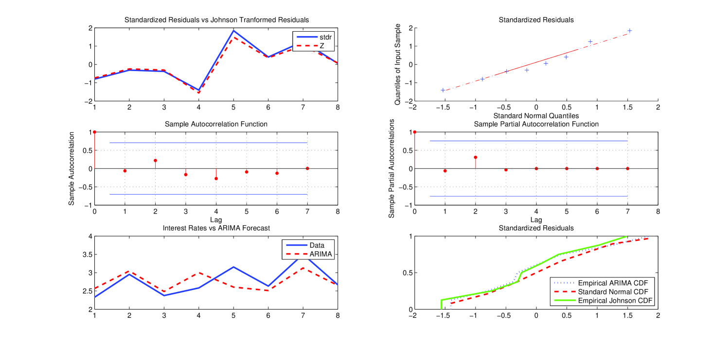
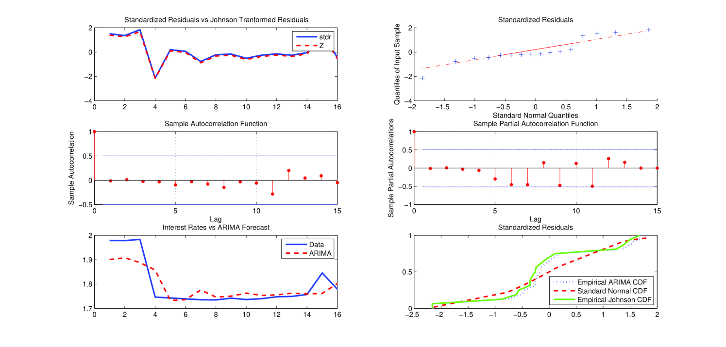
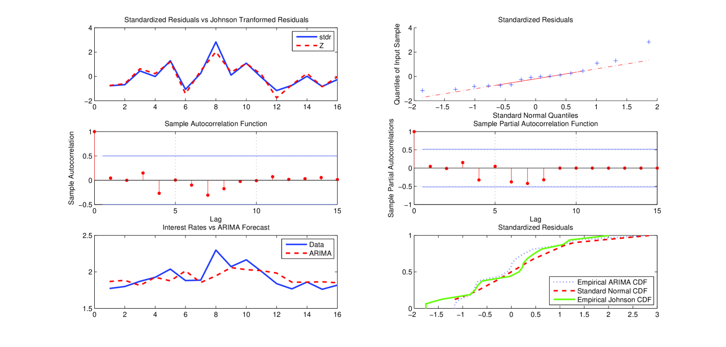
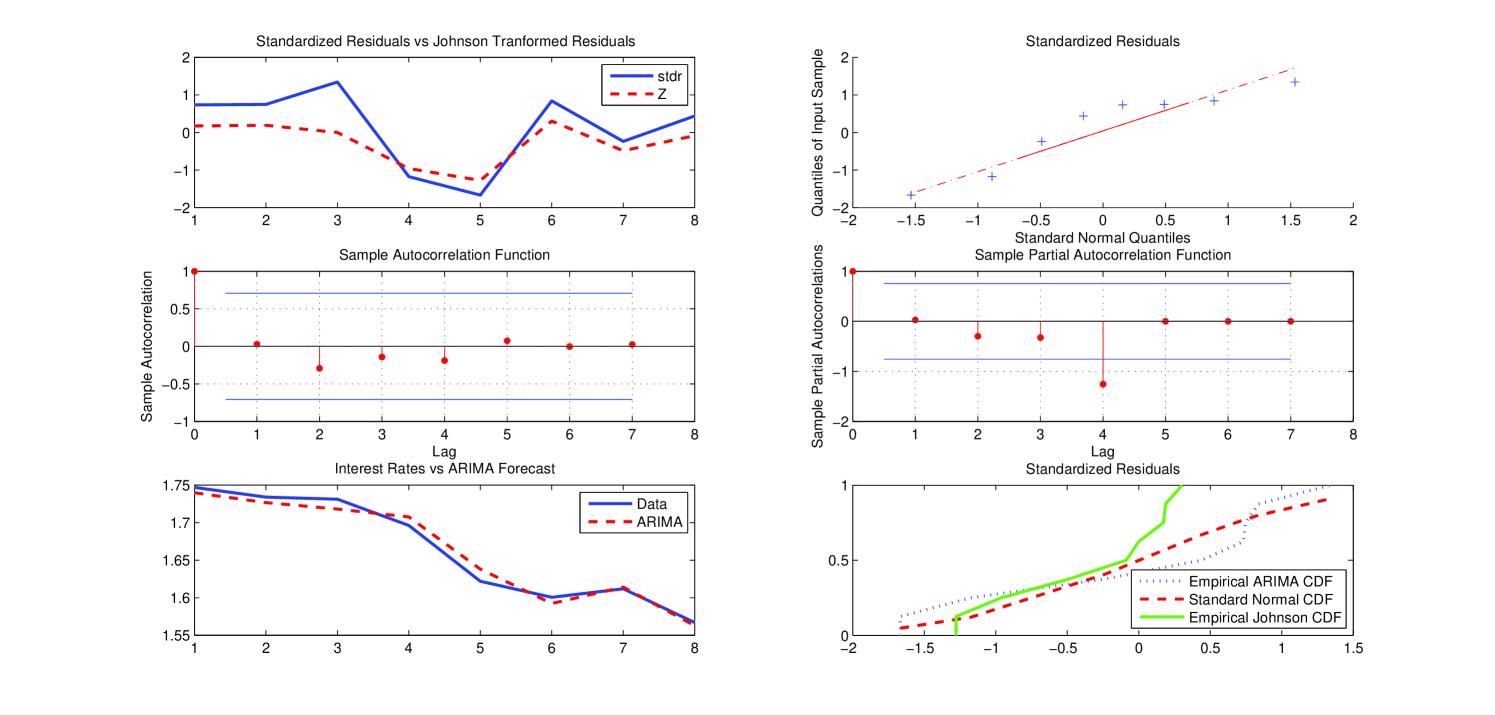
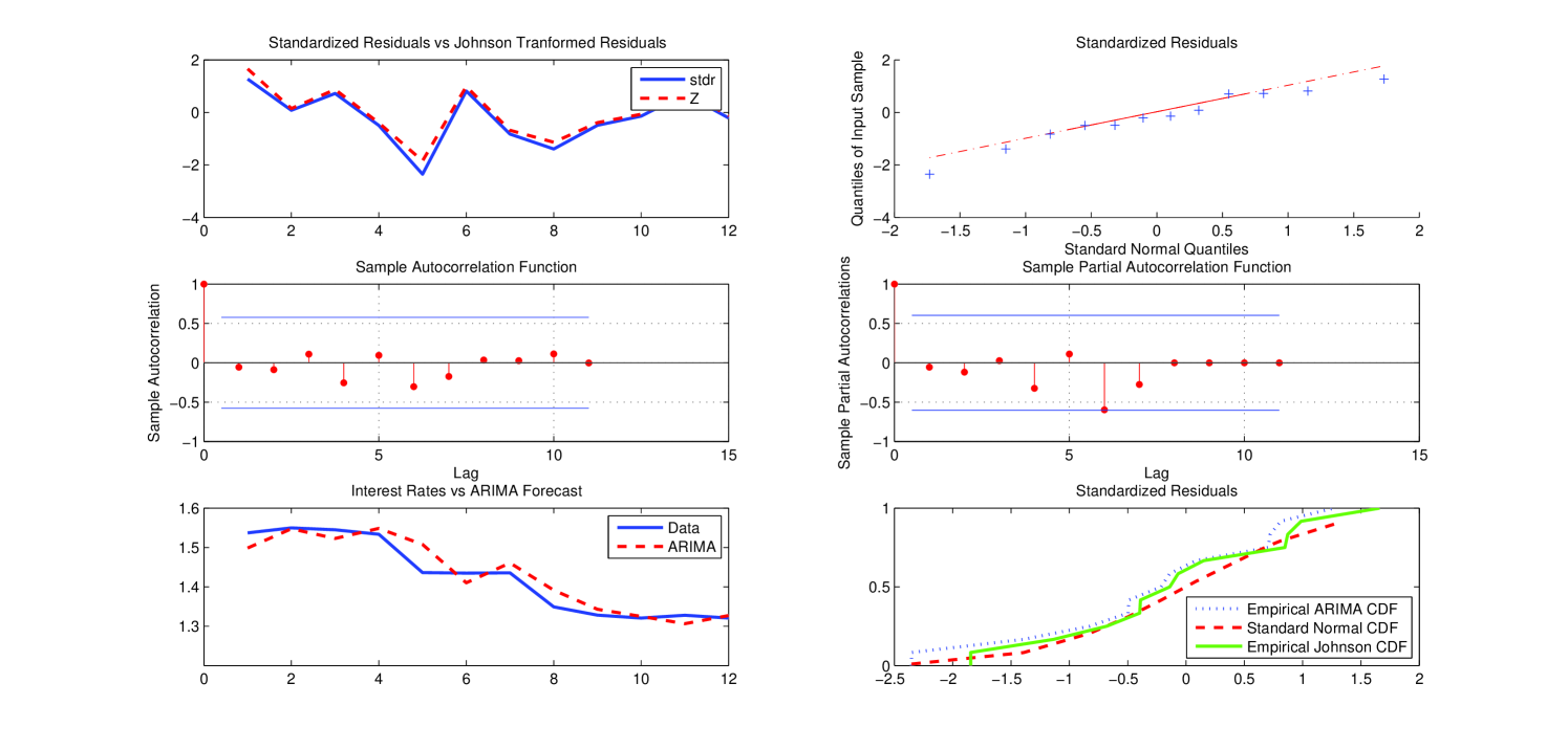
Figure 5 below reports the qualitative statistical analysis carried out by applying the ARIMA model chosen as the “optimal” forecasting model for the group 9–16 (similar plots for the other group/sub-groups are reported in A).
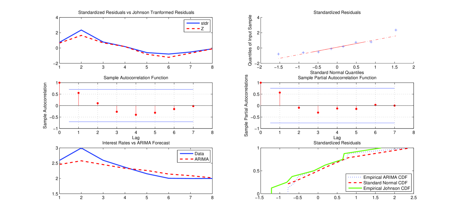
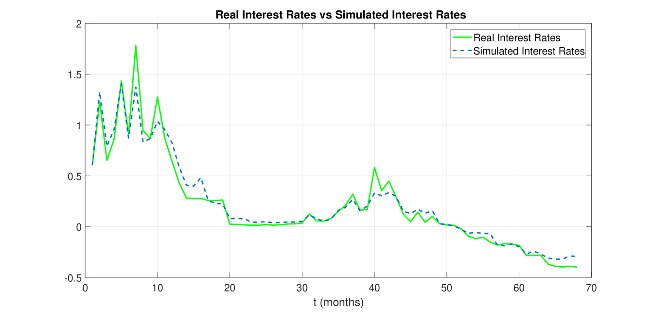
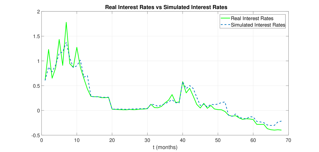
Figure 6 compares the short-term interest rates structure of the analysed market data sample with the corresponding curve of CIR fitted values computed by the simulation scheme (11) for each group partitioning the whole data sample. It is worth noting that the normally distributed standardized residuals of the “optimal” ARIMA-CIR model selected for each group/sub-group (see Table 3) replace the realizations of a standard Brownian motion in (11). This strategy allows us to get an exact trajectory of CIR fitted values instead of a curve averaged over 100,000 simulated trajectories. Consequently, the computational cost is considerably reduced.
The real interest rates have been shifted by using a translation of type (5), where corresponds to the -percentile of the conditional distribution of the spot rates process, as described in Section 4.3. Finally, the CIR fitted values have been shifted back.
The total values of the statistics and the RMSE have been computed on the whole sample as a weighted mean of the and values corresponding to the “optimal” ARIMA model chosen for each group/sub-group, i.e.
| (13) |
4.6 The change points detection problem
As explained in Section 4.2, where we have partitioned the available market data sample in groups with an arbitrary fixed length, say , the main difficulty concerns the choice of the optimal segmentation to detect abrupt changes in the variance of the interest rates dynamics. In the literature there exist several approaches for detecting multiple changes in the probability distribution of a stochastic process or a time series such as sequential analysis (i.e., “online” methods), clustering based on maximum likelihood estimation (i.e. “offline” methods), minimax change detection, etc. (see, for example, Bai and Perron (2003) [3], Lavielle (2005) [24] and (2006) [25], Hacker and Hatemi-J (2006)[15], Adams and MacKay (2007) [1], Arlot and Cenisse (2011) [2]).
| - compute the array of change points detected in the real data array |
| by the Lavielle method |
| - set ; |
| - initialize , ; |
| ( denote the first and last component of a partitioning group |
| at each processing cycle) |
| - initialize ; |
| - set +1 (each group must have a minimum length equal to )1; |
| - while & |
| - compute and the matrix |
| ( is the matrix of possible ARIMA for ); |
| - if |
| - compute ; |
| - if |
| - compute and |
| - let |
| ( is the array of the rescaled change points, see Figure 7 ); |
| - set ; |
| - set ; |
| - set ; |
| - set ; |
| - else |
| - set |
| - set ; |
| - end |
| - end |
| - if |
| - if |
| - set ; |
| - else ; |
| - end |
| - end |
| - end |
-
1
Some statistical tests (involved in ) require a minimum sample length equal to , so one can also set .
In this work we decided to implement the Matlab algorithm proposed by Lavielle (2005) [24] for the detection of changes in the variance, which led to partitioning the real data sample into the following six groups: 1–13, 14–19, 20–30, 31–39, 40–52, 53–68. However, taking into account that our CIR# model is based on the combination of an ARIMA model and the original CIR model, the above detected change points reported in Figure 7, namely 13, 19, 34, 39, 52, have to be adjusted according to the numerical scheme described in Table 4.

Table 5 lists the results from the ARIMA-CIR algorithm after application of the change point detection algorithm. Figure 8 plots the real interest rates versus the CIR# fitted values according to results in Table 5. We found that the total and the total RMSE . As before, for all , the errors are at most of the order of .
| j | Groups | ARIMA model | BIC cond. | ||
|---|---|---|---|---|---|
| 1 | 1–13 | (2,1,1) | 0.6223 | 0.2251 | |
| (3,1,1) | 0.6117 | 0.2258 | |||
| (3,1,2) | 0.5985 | 0.2299 | |||
| 2 | 14–19 | (1,0,1) | 0.8842 | 0.0048 | |
| (2,0,1) | 0.7960 | 0.0062 | |||
| (2,0,2) | 0.8814 | 0.0047 | |||
| (2,0,3) | 0.8795 | 0.0047 | |||
| (1,1,1) | 0.8291 | 0.0058 | |||
| (1,1,2) | 0.8821 | 0.0048 | |||
| (1,2,1) | 0.7623 | 0.0068 | |||
| (2,1,1) | 0.8421 | 0.0055 |
| j | Groups | ARIMA model | BIC cond. | ||
| 3 | 20–30 | (3,1,2) | 0.6345 | 0.0087 | |
| (3,1,3) | 0.6193 | 0.0089 | |||
| (1,2,3) | 0.6452 | 0.0099 | |||
| (2,2,2) | 0.5178 | 0.0096 | |||
| (2,2,3) | 0.5777 | 0.0089 | |||
| (3,2,2) | 0.6369 | 0.0085 | |||
| 4 | 31–39 | (1,0,1) | 0.7165 | 0.0444 | |
| (1,0,2) | 0.6895 | 0.0465 | |||
| (1,0,3) | 0.6815 | 0.0469 | |||
| (1,1,1) | 0.7168 | 0.0439 | |||
| (1,1,2) | 0.7247 | 0.0415 | |||
| (1,1,3) | 0.5409 | 0.0546 | |||
| (2,1,1) | 0.6876 | 0.0458 | |||
| (2,1,2) | 0.7478 | 0.0404 | |||
| (2,1,3) | 0.6778 | 0.0449 | |||
| (1,2,3) | 0.5911 | 0.0507 | |||
| (2,2,3) | 0.5817 | 0.0509 | |||
| (3,2,2) | 0.6379 | 0.0473 | |||
| 5 | 40–52 | (1,0,2) | 0.8841 | 0.1050 | |
| (2,0,1) | 0.8868 | 0.1196 | |||
| (2,0,2) | 0.7985 | 0.1317 | |||
| (2,0,3) | 0.7979 | 0.1315 | |||
| (3,0,1) | 0.8944 | 0.1178 | |||
| (3,0,2) | 0.8186 | 0.1230 | |||
| (3,0,3) | 0.8786 | 0.1158 | |||
| (1,1,1) | 0.6359 | 0.1653 | |||
| (1,1,2) | 0.6004 | 0.1752 | |||
| (1,1,3) | 0.6436 | 0.1595 | |||
| (2,1,1) | 0.8459 | 0.1287 | |||
| (2,1,2) | 0.5547 | 0.1783 | |||
| (2,2,1) | 0.6694 | 0.1637 | |||
| (3,2,3) | 0.7306 | 0.1630 | |||
| 6 | 53–68 | (1,0,3) | 0.8111 | 0.0683 |
5 Forecast of future interest rates
In this section we will address briefly the CIR# model’s progress on future interest rate forecasts from a window of observed market data. Ex-ante forecasts require a thorough analysis and will be extensively treated in a forthcoming research. It is worth noting that in this work we decided to impose the most challenging conditions by modelling the shortest part of the yield curve (e.g. the overnight rate) and using only a handful of number of observations. For instance, with monthly data we have found that observations are sufficient for a good calibration. Thus we start to consider a fixed size window of 8 real interest rates that is rolled through time, each month adding the new rate and taking off the oldest rate. The length of this window (8 months) is the historical period over which we forecast the next-month spot rate value. The numerical procedure described in Sections 4.3–4.5 has been applied to forecast future next-month interest rates based on monthly EUR interest rates with overnight maturity. The predicted curve is shown in Figure 9, compared with the real observed term structure.
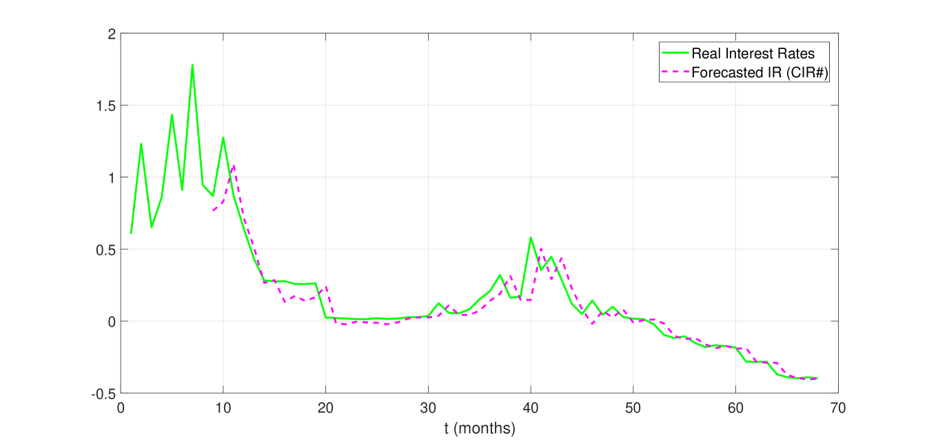
It is evident that the predicted next-month spot rates computed by the CIR# model follow the market trend. Moreover, the values of and RMSE computed to measure the goodness-of-fit of forecast interest rates to real data, are respectively and .
5.1 CIR# forecasts versus CIR forecasts
Here we are going to analyze the CIR# improvements in forecast as compared to the original CIR model. It is worth noting that calibrating the CIR parameters to real data, a hystorical window of observations is usually needed. To do that, herein we applied the martingale estimating functions method for diffusion processes proposed by Bibby et al. [4, Example 5.4](2005), which shows a better performance with respect to the Maximum Likelihood approach, as empirically confirmed in [31]. In this case, to forecast a next-month rate by the standard CIR model the minimum length of a rolling window is , against the window size of observations, required by the CIR#. Figure 10 illustrates the future next-month values predicted by the CIR# compared with the ones forecasted by the classical model, showing a better fitting to the real observed term structure.
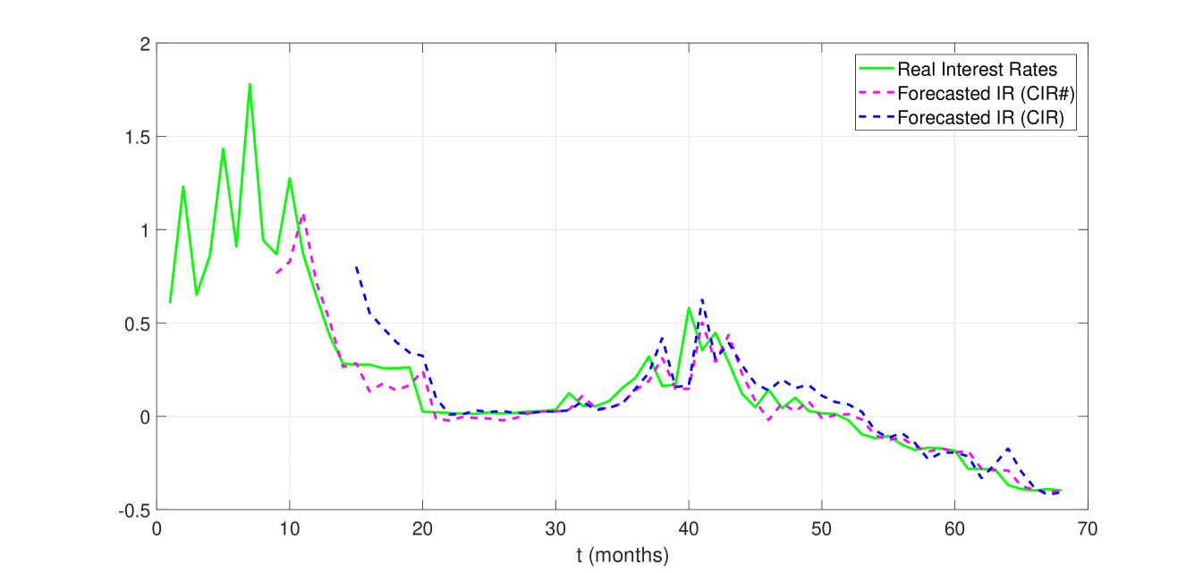
The values of and , listed in Tables 6 and 7 for ten term structures ranging from maturity day to days, confirm the improvement of the proposed novel model compared to the original one applied to shifted data.
| A | B | C | D | |
| Maturity | Difference | Performance | ||
| CIR# | CIR | A-B | C/A | |
| 1 d | 0.8082 | 0.6279 | 0.1803 | 22.38% |
| 30 d | 0.9506 | 0.9232 | 0.0274 | 2.88% |
| 60 d | 0.9676 | 0.9234 | 0.0445 | 4.59% |
| 90 d | 0.9674 | 0.9343 | 0.0332 | 3.43% |
| 120 d | 0.9705 | 0.9090 | 0.0615 | 6.33% |
| 150 d | 0.9735 | 0.9533 | 0.0202 | 2.07% |
| 180 d | 0.9752 | 0.9567 | 0.0185 | 1.89% |
| 210 d | 0.9758 | 0.9588 | 0.0170 | 1.74% |
| 240 d | 0.9782 | 0.9589 | 0.0193 | 1.97% |
| 270 d | 0.9735 | 0.9589 | 0.0146 | 1.49% |
| A | B | C | D | |
| Maturity | Difference | Performance | ||
| CIR# | CIR | A-B | C/A | |
| 1 d | 0.0963 | 0.1416 | -0.0453 | 47.04% |
| 30 d | 0.0463 | 0.0576 | -0.0113 | 24.40% |
| 60 d | 0.0406 | 0.0628 | -0.0222 | 54.67% |
| 90 d | 0.0476 | 0.0675 | -0.0199 | 41.80% |
| 120 d | 0.0484 | 0.0851 | -0.0367 | 75.82% |
| 150 d | 0.0488 | 0.0646 | -0.0158 | 32.37% |
| 180 d | 0.0500 | 0.0660 | -0.0160 | 32.00% |
| 210 d | 0.0511 | 0.0667 | -0.0157 | 30.72% |
| 240 d | 0.0503 | 0.0689 | -0.0186 | 36.97% |
| 270 d | 0.0570 | 0.0709 | -0.0139 | 24.38% |
6 Conclusions
Several different extensions of the original model have been proposed to date, with the aim of overcoming the limitations of the CIR model: from one-factor models including time-varying coefficients or jump diffusions to multi-factor models. All these extensions preserve the positivity of interest rates but, in some cases, the analytical tractability of the basic model is violated. Our approach, instead, is based on a proper translation of interest rates such that the market volatility structure is maintained as well as the analytical tractability of the original CIR model. Thus the suggested CIR# model is quite powerful for the following reasons. First, all the improvements are obtained within the CIR framework in order to preserve the single-factor property and the analytical tractability of the original model. Second, market interest rates are properly translated away from zero and/or negative values. The market data sample is partitioned into sub-groups in order to capture all the statistically significant changes of variance in real spot rates and therefore gives an account of jumps. Third, we have introduced a new way of calibration of the CIR model parameters to actual data. The standard Brownian motion process in the random part of the model is replaced with normally distributed standardized residuals of “optimal” ARIMA models suitably chosen. As a result, exact CIR fitted values to real data are calculated and the computational cost of the numerical procedure is considerably reduced. Fourth, we have shown that the CIR# model is efficient and able to follow very closely the structure of market short-term interest rates (especially for short maturities that, notoriously, are very difficult to handle) and to predict future interest rates better then the original CIR model. As a measure of goodness-of-fit, we obtained high values of the statistics and small values of the square error for each sub-group and the entire data sample. Future research will show the predictive power of the model by extending the dataset in terms of frequency and size.
References
References
- [1] R.P. Adams and D.J. MacKay, Bayesian Online Changepoint Detection, arXiv:0710.3742, 2007;
- [2] S. Arlot and A. Celisse, Segmentation of the Mean of Heteroscedastic Data Via Cross-Validation, Statistics and Computing 21(4), 2011, 613-632 ;
- [3] J. Bai and P. Perron, Computation and Analysis of Multiple Structural Change Models, Journal of Applied Econometrics 18(1), 2003, 1-22;
- [4] B.M. Bibby, M. Jacobsen and M. Sørensen, Estimating Functions for Discretely Sampled Diffusion Type Models. In Y. Aït-Sahalia and L. P. Hansen (Eds.) Handbook of Financial Econometrics 1, 2010, 203-268;
- [5] BIS, Is the Unthinkable Becoming Routine?, Technical Report, Bank for International Settlements, 2015;
- [6] D. Brigo and N. El-Bachir, Credit Derivatives Pricing with a Smile-Extended Jump Stochastic Intensity Model. Available at SSRN 950208, 2007, doi: 10.2139/ssrn.950208;
- [7] D. Brigo and F. Mercurio, A Deterministic-Shift Extension of Analytically-Tractable and Time-Homogeneous Short Rate Models, Finance and Stochastics 5, 2001, 369-388;
- [8] D. Brigo and F. Mercurio, Interest Rate Models-Theory and Practice. With Smile, Inflation and Credit, Springer-Verlag, Berlin, Heidelberg, 2006;
- [9] R.A. Carmona and M.R. Tehranchi, Interest Rate Models: an Infnite Dimensional Stochastic Analysis Perspective, Springer-Verlag, Berlin, Heidelberg, 2006;
- [10] L. Chen, Stochastic Mean and Stochastic Volatility - A Three-Factor Model of the Term Structure of Interest Rates and Its Applications in Derivatives Pricing and Risk Management, Financial Markets, Institutions & Instruments 5, 1996, 1-88;
- [11] J.C. Cox, J.E. Ingersoll and S.A. Ross, A Theory of the Term Structure of Interest Rates, Econometrica 53, 1985, 385-407;
- [12] D. Duffie, Credit Risk Modeling with Affine Processes, Journal of Banking and Finance 29(11), 2005, 2751-2802;
- [13] D. Duffie, D. Filipović and W. Schachermayer, Affine Processes and Applications in Finance, Annals of Applied Probability 13(3), 2003, 984-1053;
- [14] K.C. Engelen, The Unthinkable as the New Normal, The International Economy 29(3), 2015;
- [15] R.S. Hacker and A. Hatemi-J, Tests for Causality between Integrated Variables Using Asymptotic and Bootstrap Distributions: Theory and Application, Applied Economics 38(13), 2006, 1489-1500;
- [16] S.L. Heston, A Closed-Form Solution for Options with Stochastic Volatility with Applications to Bond and Currency Options, The Review of Financial Studies 6(2), 1993, 327-343;
- [17] J.C. Hull and A. White, Pricing Interest-Rate-Derivative Securities, The Review of Financial Studies 3(4), 1990, 573-592;
-
[18]
IBA. Data Vendor Codes. ICE Benchmark Administration (IBA)
https://www.theice.com/publicdocs/IBA_Quote_Vendor_Codes.xlsx; - [19] M. Jeanblanc, M. Yor and M. Chesney, Mathematical Methods for Financial Markets, Springer, New York, 2009;
- [20] N.L. Johnson, Systems of Frequency Curves Generated by Methods of Translation, Biometrika 36(1/2), 1949, 149-176;
- [21] D.L. Jones, The Johnson Curve Toolbox for Matlab: Analysis of Non-Normal Data Using the Johnson System of Distributions, College of Marine Science, University of South Florida, St. Petersburg, Florida, USA, 2014;
- [22] M. Keller-Ressel and T. Steiner, Yield Curve Shapes and the Asymptotic Short Rate Distribution in Affine One-Factor Models, Finance and Stochastics 12(2), 2008, 149-172;
- [23] T.O. Kvalseth, Cautionary Note about , The American Statistician 39(4), 1985, 279-285;
- [24] M. Lavielle, Using Penalized Contrasts for the Change-Point Problem, Signal Processing 85(8), 2005, 1501-1510;
- [25] M. Lavielle and G. Teyssiere, Detection of Multiple Change-Points in Multivariate Time Series, Lithuanian Mathematical Journal 46(3), 2006, 287-306;
- [26] G. Milshtein, A Method of Second-Order Accuracy Integration of Stochastic Differential Equations, Theory of Probability and Its Applications 23(2), 1979, 396-401;
- [27] M. Moreno and F. Platania, A Cyclical Square-Root Model for the Term Structure of Interest Rates, European Journal of Operational Research 241(1), 2015, 109-121;
- [28] A.R. Najafi and F. Mehrdoust, Bond Pricing Under Mixed Generalized CIR Model with Mixed Wishart Volatility, Journal of Computational and Applied Mathematics 319(C), 2017, 108-116;
- [29] A.R. Najafi, F. Mehrdoust and S. Shirinpour, Pricing American Put Option on Zero-Coupon Bond under Fractional CIR Model with Transaction Cost, Communications in Statistics - Simulation and Computation 0(0), 2017, 1-7;
- [30] G. Orlando, R. M. Mininni and M. Bufalo, A New Approach to CIR Short-Term Rates Modelling. In M. Mili, F. di Pietro and R. Samaniego Medina (Eds.), New Methods in Fixed Income Modeling, Springer International (USA),2018 (to appear);
- [31] G. Orlando, R. M. Mininni and M. Bufalo, On the Forecast of Expected Short-Term Interest Rates in the CIR Model,Preprint 2018;
- [32] G. Orlando and G. Taglialatela, A Review on Implied Volatility Calculation, Journal of Computational and Applied Mathematics 320, 2017, 202-220;
- [33] L. Rogers, Gaussian errors, Risk 9(1), 1996, 42-45;
- [34] O. Vasicek, An Equilibrium Characterization of the Term Structure, Journal of Financial Economics 5(2), 1977, 177-188;
- [35] L. Zhu, Limit Theorems for a Cox-Ingersoll-Ross Process with Hawkes Jumps, Journal of Applied Probability 51(3), 2014, 699-712;
Appendix A Qualitative analysis related to Table 3
We report the qualitative statistical analysis carried out for each group/sub group according to the results reported in Table 3. The qualitative analysis related to the results in Table 5 is analogous and so it is omitted.
Appendix B CIR parameter estimates
We report the estimates of the CIR parameters and, in particular, the plots of the function defined in (8), corresponding to the selected “optimal” ARIMA models reported in Table 3.
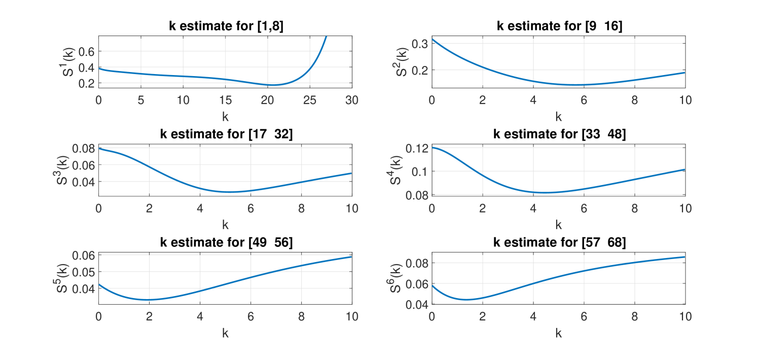
| j | group/sub-group | |||
|---|---|---|---|---|
| 1 | 1–8 | 20.6364 | 2.7699 | 0.4027 |
| 2 | 9–16 | 5.6621 | 2.3338 | 0.3663 |
| 3 | 17–32 | 5.1649 | 1.7924 | 0.0954 |
| 4 | 33–48 | 4.4462 | 1.9223 | 0.1546 |
| 5 | 49–56 | 1.9092 | 1.6637 | 0.0709 |
| 6 | 57–68 | 1.3555 | 1.4264 | 0.0958 |