PromiseNP
On the Complexity of Restoring Corrupted Colorings††thanks: Work partially supported by the Emil Aaltonen Foundation (J.L).
Abstract
In the -Fix problem, we are given a graph , a (non-proper) vertex-coloring , and a positive integer . The goal is to decide whether a proper -coloring is obtainable from by recoloring at most vertices of . Recently, Junosza-Szaniawski, Liedloff, and Rzążewski [SOFSEM 2015] asked whether the problem has a polynomial kernel parameterized by the number of recolorings . In a full version of the manuscript, the authors together with Garnero and Montealegre, answered the question in the negative: for every , the problem -Fix does not admit a polynomial kernel unless . Independently of their work, we give an alternative proof of the theorem. Furthermore, we study the complexity of -Swap, where the only difference from -Fix is that instead of recolorings we have a budget of color swaps. We show that for every , the problem -Swap is -hard whereas -Fix is known to be FPT. Moreover, when is part of the input, we observe both Fix and Swap are -hard parameterized by treewidth. We also study promise variants of the problems, where we are guaranteed that a proper -coloring is indeed obtainable from by some finite number of swaps. For instance, we prove that for , the problems -Fix-Promise and -Swap-Promise are -hard for planar graphs. As a consequence of our reduction, the problems cannot be solved in time unless the Exponential Time Hypothesis (ETH) fails.
1 Introduction
Computational models are sometimes too idealized, and do not capture all information available or relevant to a problem. Moreover, in a dynamic world, constraints change over time due to more information becoming available. A problem arising frequently in practice in e.g., scheduling [27] is graph coloring. An assignment of colors to the vertices of a graph is an -coloring. Formally, an -coloring is said to be proper if for every . In the graph coloring problem, the goal is to find the smallest for which a graph is -colorable. This quantity is known as the chromatic number of , and is denoted by . Graph coloring is one of the most central problems in discrete mathematics and optimization. For a general introduction to the topic, we refer the reader to the book [17].
Suppose we have a graph for which we have computed a proper vertex-coloring using colors. Then due to constraints changing, a malicious adversary, or e.g., a system failure, the coloring is corrupted by redistributing the vertex colors over the graph . How hard is it to restore the corrupted coloring to some optimal proper coloring of ? In 2006, Clark, Holliday, Holliday, Johnson, Trimm, Rubalcaba, and Walsh [5] introduced and investigated this problem under the name chromatic villainy. For restoring a corrupted coloring, they used the following operation called a swap. A swap between two distinct vertices and is the operation of assigning to the color that appears on , and vice versa. Formally, let be a vertex-coloring of a graph . The villainy of , denoted by , is the minimum number of swaps to be performed to transform into some proper vertex-coloring of . The quantity can also be seen as the minimum number of recolorings with the constraint that each color used in the new coloring must be used the same number of times as in . In addition to the graph-theoretic viewpoint, there has been interest in the computational aspects of chromatic villainy [31].
Very recently, Junosza-Szaniawski, Liedloff, and Rzążewski [20] studied a problem they call -Fix. In the problem, we are given a graph , a non-proper -coloring of , and an integer . The task is to decide whether a proper vertex-coloring is obtainable from using at most vertex recolorings. The authors observe the problem is -complete, and give several positive complexity results as well. In particular, using the framework of Björklund, Husfeldt, and Koivisto [1] they obtain a -time and exponential space algorithm, where is the number of vertices in the input graph. Furthermore, they show that for any fixed , the problem is fixed-parameter tractable (FPT) parameterized by the number of recolorings . Finally, in the same paper, the authors show that for graphs of treewidth , the problem can be solved in time. For a discussion on several related reoptimization and reconfiguration problems, we refer the reader to [20]. We also note that their results are considerably expanded in a full version of the manuscript currently under review [13].
The main difference between -Fix and chromatic villainy as defined by Clark et al. [5] is the basic operation used. In -Fix it is a recoloring, whereas in chromatic villainy it is a swap. For this reason, we shall refer to the computational problem arising from chromatic villainy as -Swap. That is, the input to -Swap is exactly the same as it is in -Fix, but instead of recolorings we have a budget of swaps. Strictly speaking, there is another difference. In fact, in chromatic villainy, the corrupted vertex-coloring is not an arbitrary one, but has an additional property that could possibly be exploited. Namely, the property is that by using some finite number swaps, a proper vertex-coloring is indeed obtainable from the given one. Additional promises of properties of a problem are captured by the notion of a promise problem. Promise problems were introduced and studied by Even, Selman, and Yacobi [9], and they have several applications (for a survey, see [14]). In fact, it seems fair to argue that promise problems model real-world problems more accurately. Indeed, Goldreich [14] writes: “… I contend that almost all readers refer to this notion when thinking about computational problems, although they may be often unaware of this fact”. Motivated by these facts, we also separate two additional problems, -Fix-Promise and -Swap-Promise, for which the input is guaranteed to satisfy additional properties (a precise definition is provided in Section 2).
In this context, it is natural to investigate whether a hard problem becomes easy when the set of instances is restricted. A priori, it is unknown how the addition of a promise affects the computational complexity of a problem. For example, it is hard to decide whether a graph contains a Hamiltonian cycle, even if we are promised it contains at most one such cycle [18]. In the other direction, one can efficiently find a satisfying assignment for an -variable SAT formula that promises to have at least satisfying assignments. However, as shown by Valiant and Vazirani [30], it is hard to find an assignment even when the formula is promised to have exactly one solution.
Motivation. The problems -Fix and -Swap are tightly related to local search which is a core technique in solving combinatorial optimization and operations research problems in practice. In local search, one aims to improve upon the current solution by replacing it with a better solution in its neighborhood. Specifically, the neighborhood is defined by the set of allowed operations that modify the current solution. Plausibly, the larger the neighborhood, the less likely is the local search to get stuck in a local optimum. On the other hand, the allowed operations should not be too demanding to compute. In fact, there has been significant interest in applying methods from parameterized complexity to analyzing local search procedures (see e.g., [21, 23, 11, 29, 7]).
The studied problems are also related to combinatorial reconfiguration problems, in particular -coloring reconfiguration [19, 4, 32]. In this problem, we are given two proper -colorings for a graph, and asked whether one can be transformed into the other by changing one color at a time, maintaining a proper coloring throughout. We argue that in the context of local search, the property of maintaining a proper -coloring at each step can be relaxed: we are only interested in eventually arriving at a solution. To further motivate the use of promise conditions, we remark that there are -coloring problems in which we know the sizes of the color classes (if an -coloring exists). These include well-known problems arising from coding theory, such as partitioning of the -dimensional Hamming space into binary codes with certain properties [28].
Our results. We continue the investigation of the complexity of restoring corrupted colorings. Specifically, we further study the complexity of -Fix, under different basic operations and/or promise conditions.
-
•
For Section 3, our main result is that for any fixed , the problem -Swap is -hard parameterized by the number of swaps . Moreover, the same is true for -Swap-Promise. This should be contrasted with the positive FPT result of Junosza-Szaniawski et al. [20] for -Fix. In addition, we observe both problems -Fix and -Swap become -hard for treewidth when the number of colors is part of the input. The constructions exhibit gadget ideas we use for the sections to follow.
-
•
In Section 4, we prove that under plausible complexity assumptions, -Fix has no polynomial kernel parameterized by the number of recolorings , for every . We stress that while mentioned as an open problem in [20], the question was subsequently answered by Garnero, Junosza-Szaniawski, Liedloff, Montealegre, and Rzążewski in a full version [13] of [20]. Our result was obtained independently of their work, and uses slightly different ideas.
-
•
Finally, in Section 5, we consider the complexity of the promise variants of the problems (see Section 2 for precise definitions). We show that for , both -Swap-Promise and -Fix-Promise are -hard for planar graphs. Moreover, the problems cannot be solved in time unless the Exponential Time Hypothesis fails. On the positive side, using known results, we derive an algorithm for the problem working in time.
2 Preliminaries
All graphs in this paper are simple and undirected. For graph-theoretic notion not defined here, we refer the reader to [8]. We write to denote the set .
2.1 Promises and problem statements
A promise problem is a generalization of a decision problem, where the input is guaranteed to belong to a restricted subset among all possible inputs [15].
Definition 1 (Promise problem).
A promise problem is a pair of disjoint sets of strings , and their union is called the promise set. An algorithm decides a promise problem if for every and for every ; for strings that do not belong to the promise set the algorithm must halt, but can answer arbitrarily.
A promise problem is in , the promise extension of , if there exists a polynomial and a polynomial-time verifier such that for every there exists of length at most such that and for every and every it holds that . For a more comprehensive treatment, we refer the reader to [15].
We are then ready to formally define the problems studied in this work. For the promise variants, a coloring is said to be a permutation of a proper vertex-coloring if can be obtained from by a finite number of swaps. In other words, the sizes of the color classes of match those of an optimal proper coloring.
-Fix
Instance: A graph , an -coloring , and a positive integer .
Question: Can be made into a proper -coloring of using at most recolorings?
-Fix-Promise
Instance: A graph , an -coloring , and a positive integer .
Promise: , and is a permutation of an optimal proper vertex-coloring of .
Question: Can be made into a proper -coloring of using at most recolorings?
Note that the number of recolorings needed is precisely the minimum Hamming distance between the given coloring and a valid coloring (if existing).
Similarly, we also define -Swap and -Swap-Promise, where instead of at most recolorings we have a budget of at most swaps.
-Swap
Instance: A graph , an -coloring , and a positive integer .
Question: Can be made into a proper -coloring of using at most swaps?
-Swap-Promise
Instance: A graph , an -coloring , and a positive integer .
Promise: , and is a permutation of an optimal proper vertex-coloring of .
Question: Can be made into a proper -coloring of using at most swaps?
At first glance, the promise conditions might seem to make the two problems -Fix-Promise and -Swap-Promise similar: one could think that two recolorings correspond to a swap because if we recolor a vertex, then by the promise, the color must be reinserted elsewhere. However, it is easy to build graphs in which this does not hold. For example, consider a graph constructed from a triangle with the vertices , , colored , , , respectively. Also, connect vertices to such that has three pendants (neighbours) colored and three pendants colored ; has three pendants colored and three pendants colored ; and has three pendants colored and three pendants colored . Clearly, three recolorings are enough to get a proper coloring. Indeed, we color with , with , and with , and are done. In contrast, in the swap variant, two swaps needed (e.g., swap colors on and , and then colors on and ).
2.2 FPT-reductions and (kernelization) lower bounds
In this subsection, we briefly review the necessary basics of parameterized complexity.
Definition 2.
Let be parameterized problems. A parameterized reduction from to is an algorithm such that given an instance of , it outputs an instance of such that
-
1.
is a YES-instance of iff is a YES-instance of ,
-
2.
for some computable function , and
-
3.
the running time is for some computable function .
In the Clique problem, we are given a graph and an integer . The task is to decide whether contains a complete subgraph on vertices. The class of problems reducible to Clique under parameterized reductions is denoted by . We define hardness and completeness analogously to classical complexity, but assume parameterized reductions. That is, a problem is said to be -hard if Clique (and thus each problem in ) can be reduced to it by a parameterized reduction. It is widely believed that .
Let us recall the well-known Exponential Time Hypothesis (ETH), which is often the assumption used for excluding the existence of algorithms that are considerably faster than e.g., brute-force.
Conjecture 3 (Exponential Time Hypothesis [16]).
There exists a constant , such that there is no algorithm solving -SAT in time , where is the number of variables.
Suppose is an instance of -SAT with variables and clauses. It holds that if there is a linear reduction from -SAT to, say, a graph problem , then the problem cannot be solved in time , where and denote the number of vertices and edges, respectively. Similar reasoning can be applied for -hard problems. For instance, it is known that there is no -time algorithm for Independent Set for any computable function , unless ETH fails. Then the existence of a parameterized reduction with a linear parameter dependence from Independent Set to a problem implies a lower bound for under ETH. For more examples and discussion, we refer the reader to [6, 25].
Finally, let us then mention the machinery we use to obtain kernelization lower bounds later on (for more details, see [2, 6]).
Definition 4.
An equivalence relation on is a polynomial equivalence relation if (1) there is an algorithm that given two strings decides whether in time; and (2) for any finite set the equivalence relation partitions the elements of into at most classes.
Definition 5 (Cross-composition).
Let and let be a parameterized problem. We say cross-composes into if there is a polynomial equivalence relation and an algorithm which, given strings belonging to the same equivalence class of , computes an instance in time polynomial in such that (1) iff for some ; and (2) is bounded polynomially in .
Theorem 6 ([2]).
Assume that an -hard language cross-composes into a parameterized language . Then does not admit a polynomial kernel, unless and the polynomial hierarchy collapses.
3 Parameterized aspects of restoring corrupted colorings
Junosza-Szaniawski et al. [20] focused on the -Fix problem, that is, the number of colors in the coloring is fixed to be . Among other results, they showed the problem is FPT parameterized by treewidth. In other words, the Fix problem (same as -Fix but is part of the input) is FPT for the combined parameter , where is the treewidth of the input graph. In contrast, we observe the problem is -hard when the parameter is only treewidth.
In the Precoloring Extension problem (PrExt), we are given a graph , a set of precolored vertices, and a precoloring of the vertices in . The goal is to decide whether there is a proper -coloring of extending the coloring (i.e., for every ). When is fixed, we call the problem -Precoloring Extension (-PrExt). Let us then proceed with the following observation.
Lemma 7.
There exists a polynomial time algorithm which given an instance of Precoloring Extension constructs an instance of Fix, such that is a YES-instance of Precoloring Extension iff is a YES-instance of Fix.
Proof.
Let be an instance of Precoloring Extension. To obtain, in polynomial time, an instance of Fix, we proceed as follows. First, let , , and set the number of recolorings . Then to each precolored vertex , we attach pendant vertices, called . Build from as follows. We color vertices in such that there are precisely vertices colored in every color . We retain the colors on the vertices in , and color each uncolored vertex with color . Observe that recolorings will not suffice to change the color of as it has pendants colored in each color distinct from . Thus, it is easy to see is a YES-instance of Precoloring Extension iff is a YES-instance of Fix.
To make the result hold for Swap, we add isolated vertices and color them so that we provide a choice of one of the colors for each of the non-precolored vertices. Finally, it is well-known the addition of vertices of degree at most 1 does not increase the treewidth of a graph. As Precoloring Extension is -hard for treewidth [10], we obtain the following.
Corollary 8.
Both problems Fix and Swap are -hard parameterized by treewidth.
Because Precoloring Extension is -complete when restricted to distance-hereditary graphs [3] (and thus for e.g., chordal graphs), we immediately observe the following.
Corollary 9.
Both problems Fix and Swap are -complete when restricted to the class of distance-hereditary graphs.
The above also implies hardness for bounded cliquewidth graphs.
Junosza-Szaniawski et al. [20] proved that for every fixed , the problem -Fix is FPT parameterized by the number of recolorings. However, when the basic operation is a swap instead of a recoloring, the problem becomes hard. This is established by the following lemma. For the result, we give a parameterized reduction from the well-known Independent Set problem. In this problem are given a graph , and an integer . The goal is to decide whether contains a set of pairwise non-adjacent vertices. The problem is well-known to be -hard parameterized by .
Lemma 10.
There exists a polynomial time algorithm which given an instance of Independent Set constructs an instance of -Swap for such that is a YES-instance of Independent Set iff is a YES-instance of -Swap.
Proof.
Let . To construct the graph , begin with and . Add disjoint triangles , and color them such that and , for . For each , add a disjoint triangle . In each, color , , and . Attach pendant vertices to and color of them with color , and of them with color . For each , add the edge . For every , if and , add the edge . Finally, for each , add disjoint triangles . These disjoint triangles are colored such that , , and , where . Add the edge , for and . This completes the construction of . An example is shown in Figure 1. Let us then prove is a YES-instance of Independent Set iff is a YES-instance of -Swap.
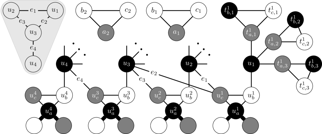
Let be an independent set. By construction, there are exactly conflicts in between and , for . Swap with , spending a total of swaps. By doing so, we fixed conflicts but also introduced new conflicts. In particular, the new conflicts are between and , as they are both colored . We swap with (colored ), and claim is properly colored. By construction, is adjacent to only if and are adjacent in . As is an independent set, each adjacent to is colored . Thus, is a proper coloring for , and we are done.
For the other direction, suppose swaps suffice to obtain a proper vertex coloring from . Again, each of the conflicts between and , for , must be fixed. To resolve the conflicts, we must swap either or with a vertex colored . Without loss, suppose we choose over . Observe that for every , we cannot swap with any vertex as it has pendant vertices colored , and pendant vertices colored . Thus, there are two possibilities: either we swap with , or with , for some and . If the swap occurs between and , we must then swap with for some . This introduces a conflict between the chosen and its adjacent vertex . After we fix this conflict, we have used a total of 3 swaps, totaling swaps if we followed this strategy for each . Thus, as swaps suffice, and we are looking for an independent set of size exactly , we must swap each of the vertices with some . Clearly, two vertices , for , adjacent in cannot be used to fix the conflicts, for otherwise we would have a conflict between the vertices and (both colored ). We conclude that the vertices a vertex is swapped with form an independent set.
By adding a properly colored -clique to the constructed graph, we can extend the lemma to cover every fixed value of . Thus, we have the following.
Theorem 11.
For every , the problem -Swap is -hard parameterized by the number of swaps . Furthermore, there is no -time algorithm for the problem unless ETH fails, where is a computable function.
In addition, it is straightforward to extend the construction of Lemma 10 to show the promise variant, namely -Swap-Promise, is -hard parameterized by the number of swaps .
Corollary 12.
For every , the problem -Swap-Promise is -hard parameterized by the number of swaps . Furthermore, there is no -time algorithm for the problem unless ETH fails, where is a computable function.
Proof.
Assume the construction of an instance of -Swap of Lemma 10. To prove the claim, it suffices to augment the construction to ensure the promise holds, i.e., that with a finite number of swaps we have that is properly -colored and .
A double star is the complete bipartite graph with each edge subdivided. Formally, . To enforce the promise, add disjoint double stars to . Each double star is colored such that the central vertex receives color 1, vertices adjacent to the central vertex color 2, and the remaining vertices color 3. Observe that after swapping the central vertex (colored 1) of a with (say) (colored 2), we require more swaps to fix the conflicts residing at that particular . Nevertheless, given enough swaps, to be precise, we can properly -color . Finally, to guarantee , it suffices to add a disjoint properly -colored clique.
4 No polynomial kernel for -Fix
Junosza-Szaniawski et al. [20] showed that for any fixed , the problem -Fix is FPT parameterized by the number of recolorings . In particular, their result implies a kernel of exponential size for the problem. Thus, they asked whether or not there is a kernel of polynomial size. The question was answered in the negative in a full version of [20] by Garnero et al. [13]. Independently of their work, in what is to follow, we give an alternative proof of the theorem.
Lemma 13.
For , the problem -Fix parameterized by the number of recolorings does not admit a polynomial kernel unless .
Proof.
We show that -SAT cross-composes into -Fix parameterized by the number of recolorings . By choosing an appropriate polynomial equivalence relation , we can assume we are given a sequence of -SAT instances with an equal number of variables, denoted by , and an equal number of clauses, denoted by .
Let us then proceed with an cross-composition algorithm that composes input instances ,, which are equivalent under into a single instance of -Fix parameterized by the number of recolorings. Specifically, we construct an instance of -Fix, where is a vertex-colored graph, and the number of recolorings. Our plan is to convert each -SAT instance to an instance of -SAT. For each resulting instance of -SAT, we apply the standard reduction from -SAT to -Coloring (see e.g., [12]). Finally, the resulting graphs are connected by a spread gadget, which acts as an instance selector. Let us first describe the gadgets, and then the construction of the whole graph . At the same time, we describe a 3-coloring . We set . Our construction depends crucially on , and its choice will become apparent later on.
3-SAT to 4-SAT. For each -SAT formula , where , introduce a new variable , and add it to each clause of . We call the resulting -SAT formula . Observe that by setting to true we satisfy .
The variable vertices. Let the variables of , where , be . We introduce disjoint 2-cliques labelled . Set and , for (i.e., initially we set each variable true). Add an isolated vertex , and let . We refer to each of the vertices as variable vertices.
The clause gadget. Denote by the th clause of . For each clause , where and , construct the following clause gadget (see Figure 2 (b)). Take three disjoint triangles , , , and add the edges , , and . We add pendant vertices adjacent to and color them with color . This guarantees recolorings cannot give color . Vertices , , and correspond to the 4 literals each clause has. Thus, we connect them to the corresponding variable vertices. That is, when corresponds to the variable , , we add the edge (and similarly when its negated). The following properties hold for a clause gadget .
-
If all four variable vertices of have color 1, then must have color 1 (costing recolorings to properly color the gadget).
-
The gadget can be properly 3-colored if one of the attached variable vertices (including ) have color 2.
The spread gadget. The spread gadget is constructed by starting from a complete binary tree on leaves with the root . We replace each internal vertex with a triangle, and attach pendant vertices to . Thus, the distance from to any leaf is . We color root , its pendant vertices, and each leaf with color . In a triangle, the top vertex receives color , the right vertex color , and the left vertex color (see Figure 2 (b)). This finishes the construction of the spread gadget.
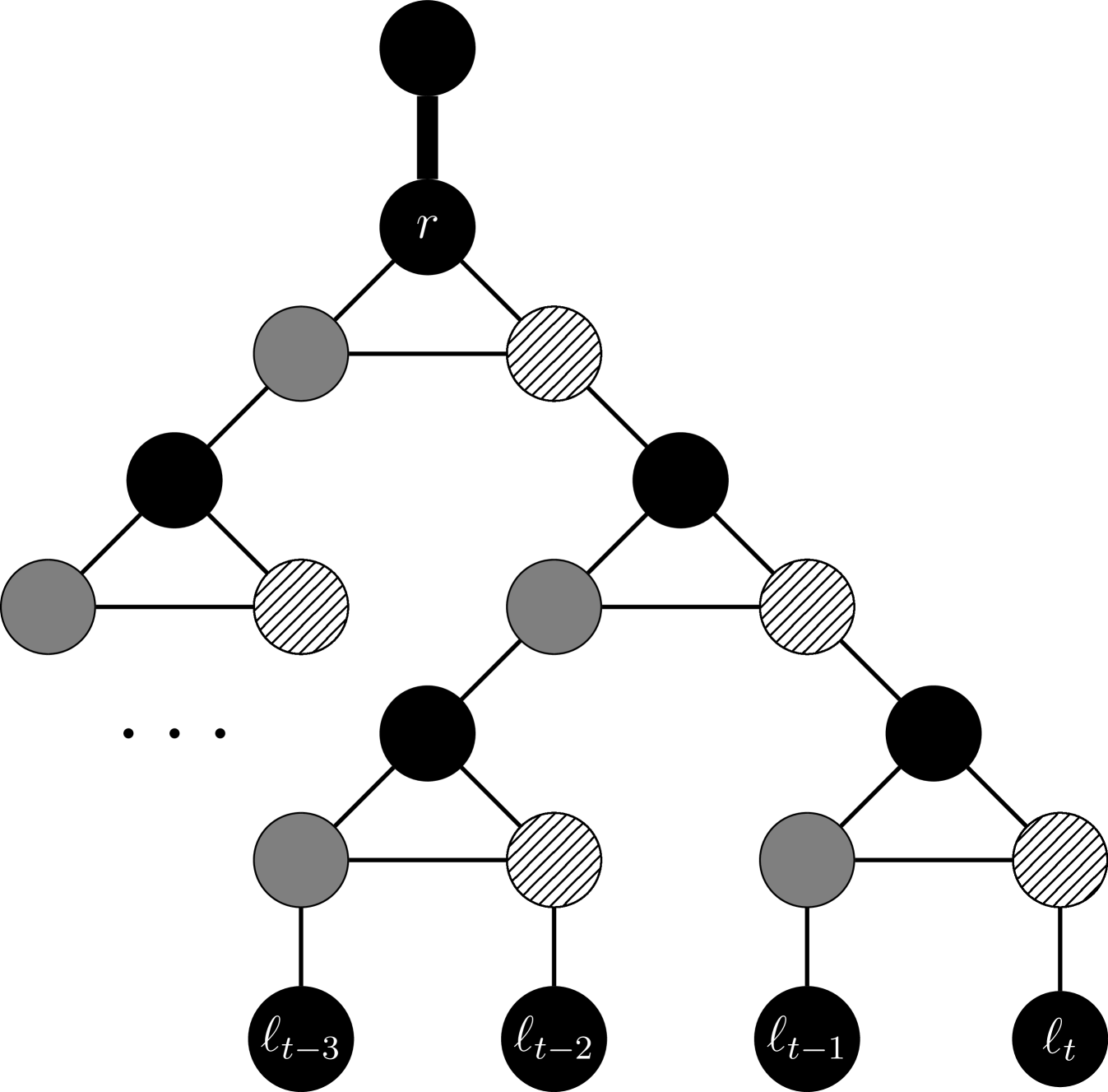
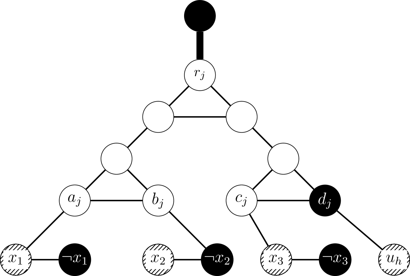
To obtain , we connect the described gadgets together as follows. For each , where , we add a vertex . Make adjacent to each variable vertex, and set . We give altogether pendant vertices, and color them so that of them have color , and of them have color . This enforces if only recolorings are available. In the spread gadget, each leaf is made adjacent to both and .
This completes the construction of the graph . Recall , and output the instance of -Fix. Let us then prove that is a YES-instance of -Fix iff one of is satisfiable for .
Correctness. Suppose is a YES-instance of -Fix. By construction, the root and its pendant vertices are colored with color in the spread gadget. As we only have a budget of recolorings, we must recolor . By doing so, we introduce a conflict into the triangle containing . When this conflict is fixed, we move it to one of the two succeeding triangles. Further continuing to fix the conflict, we propagate it down to one of the leaves , for some . Intuitively, the propagation to means we have chosen to solve the instance . By construction, forms a triangle with (colored ) and (colored ). As has pendants colored with and pendants colored with , we must move the conflict to . By moving the conflict from to , we used precisely swaps. Now, has color , as do all the vertices in . As , we have set the truth value of to false. Thus, the truth value of is not affected by the truth value of . As , each vertex in can be recolored in recolorings. Moreover, recolorings suffice to swap the color of each vertex in the three vertex-disjoint triangles a clause gadget has. By construction, the initial vertex-coloring corresponds to a truth assignment setting each variable to true. Clearly, recolorings suffice to reverse , i.e., change to such that the Hamming distance of and is . Therefore, by , if is a YES-instance of -Fix, then is satisfiable.
For the other direction, suppose is satisfiable for some . Again, the initial vertex-coloring corresponds to a truth assignment setting each variable to true. Using at most recolorings, we turn the initial vertex-coloring to a vertex-coloring corresponding to such that is satisfied under . Indeed, observe that as is satisfiable, is not violated. Moreover, observe that satisfies regardless of the truth value of . Thus, we can freely let . But now we introduce a conflict between (colored ) and its unique neighbor in the spread gadget. However, using precisely recolorings, we propagate this conflict, and in particular the color , up to the root . At most recolorings have been used, and no conflicts remain in . Thus, if at least one of is a YES-instance of -SAT, then is a YES-instance of -Fix. This concludes the proof.
In order to extend the above result to hold for every , we attach pendant vertices to each vertex of the construction. These pendant vertices are colored in the obvious way such that each “original” vertex must receive exactly one of the colors 1, 2, or 3.
Theorem 14 ([13]).
For every , the problem -Fix parameterized by the number of recolorings does not admit a polynomial kernel unless .
Note that in the light of Theorem 11, the existence of a kernel of any size depending only on and for -Swap is highly unlikely.
5 Chromatic villainy: -Swap-Promise is hard
As the main result of this section, we prove that -Swap-Promise is -hard when restricted to the class of planar graphs. In other words, even with the additional information that some proper vertex-coloring is always obtainable after a finite number of swaps (and no other proper vertex-coloring with less than 3 colors exists), the problem remains hard.
Our reduction will be from the -PrExt problem, shown to be -complete for when restricted to bipartite planar graphs by Kratochvíl [22]. In fact, although not explicitly stated, the following slightly stronger result is obtained from [22].
Theorem 15 ([22]).
The -PrExt problem is -complete for when restricted to the class of bipartite planar graphs, and each precolored vertex has degree 1, that is, for every .
The reader should be aware that in the following, we use the color set instead of . This will make it more convenient to describe the coloring through modular arithmetic. We are then ready to proceed with the main result of the section.
Theorem 16.
-Swap-Promise is -hard when restricted to the class of planar graphs. Moreover, the same is true even when every swap must be between adjacent vertices.
Proof.
Let be an instance of -PrExt, where is an -vertex bipartite planar graph, a set of precolored vertices, and a precoloring of the vertices in . By Theorem 15, we may assume without loss that each (precolored) vertex in has degree 1. Our construction crucially depends on this fact. Let be a fixed color bound, and let . We will construct a graph along with its vertex-coloring such that the precoloring can be extended to a valid -coloring of iff at most swaps are needed to transform to an optimal proper vertex-coloring of , i.e., . To enforce the promise of the problem, it shall hold for that (i) it uses precisely colors, and that (ii) by using a finite number of swaps can be transformed into a proper coloring of .
Construction. Let be the set of uncolored vertices, let and be the bipartition of , that is, , and let us name the set of colors . The graph and its vertex-coloring are constructed from and its precoloring as follows.
-
•
We retain the coloring on the vertices of , that is, , for every .
-
•
If has one or more neighbors colored with color (observe it cannot have distinctly colored neighbors), we set . If all neighbors of are uncolored, we set if . Otherwise, , so we set . For each , we also add two vertices and along with the edges and . We color and .
-
•
For each precolored vertex we add new vertices and . These will be made pendant vertices of by adding the altogether edges and where . They receive a color as follows, where denotes the color of :
-
–
if , then and , where ;
-
–
if , then and , where ; and
-
–
in all other cases , and .
-
–
-
•
For every precolored vertex , we add new vertices with the edges , and set , where .
-
•
For every precolored vertex , we add new vertices with the edges , and set , where .
-
•
Finally, consider an arbitrary precolored vertex , and its set of pendant vertices . We choose an arbitrary vertex among the vertices, and call it . Then, we add two vertices and along with the edges , , and . These vertices are colored such that and .
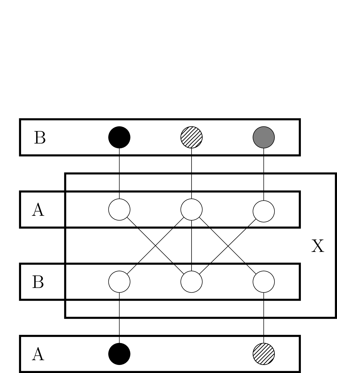
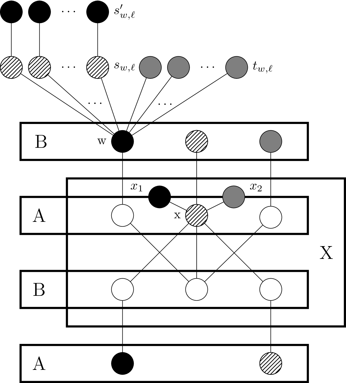
This finishes the construction of the graph along with its vertex-coloring . It is straightforward to verify is planar, but not bipartite because of the triangle on the vertices , , and . An example is shown in Figure 3. We will then prove is YES-instance of PrExt iff , that is, if swaps suffice to transform into a proper coloring of .
Correctness. Suppose can be extended to a proper vertex-coloring of . We will show swaps suffice to transform into a proper coloring of . For each , we perform a swap between and either or . Then for every it holds that either (and there is no need to swap it), or one of the two described swaps can change the color of to . Now, let be the color of before the swap, and its color after the swap. Let be the neighbors of . If was a precolored vertex, then by construction; if was an uncolored vertex then the valid coloring guarantees that . Thus, the claim follows.
For the other direction, suppose . Consider a precolored vertex and let . We claim that for any valid extension of , it holds that . More precisely, we will show that if the color of was changed, then it is impossible for to be an extension of . By construction, the vertex has neighbors each colored , and neighbors each colored with . Thus, if one swap was used to change the color on , then after swaps there would be at least one edge incident to with its endpoints having the same color. So we have that . Moreover, is completed to an extension of by picking the colors assigned to the uncolored vertices after the swaps. This completes the proof of correctness for our reduction.
Promise. Let us then show that the promise holds as well. That is, we show that can be transformed into a proper vertex-coloring of with a finite number of swaps even if the original precoloring of cannot be extended to a proper coloring (but in this case, more than swaps are needed).
First, we show that a finite number of swaps gives us a 2-coloring for such that every vertex in receives color , and every vertex in color . Afterwards, we will adjust the remaining pendant vertices , , and so that no color conflict remains.
If , then we swap it with one of its neighbors or and get . Similarly, if , a swap with either or gives us .
Let us then consider the precolored vertices. If , we swap with which is colored . This causes a conflict , which is fixed by swapping with that are colored . Similarly, if , we swap with which is colored . This causes conflicts , where . To fix them, we swap with that are colored . Thus, we have that all vertices in are colored , and all vertices in are colored . Moreover, for all we have , where . Also, , where . Thus, is a valid coloring of and the triangle guarantees that . Thus, the claim follows.
By removing the promise condition, we can modify our reduction to obtain the following.
Corollary 17.
For every , the problem -Swap is -complete for bipartite planar graphs.
Another corollary follows by a chain of reductions. First, Lichtenstein [24] gives a reduction from -SAT to Planar -SAT showing Planar -SAT cannot be solved in time , unless ETH fails. Continuing to compose reductions, Mansfield [26] gives a linear reduction from Planar -SAT to Planar -in--SAT, which is then similarly reduced by Kratochvíl [22] to -PrExt (the result of Theorem 15). Finally, it can be verified the construction of Theorem 16 has linear size, giving us the following.
Corollary 18.
There is no algorithm which solves Planar -Swap-Promise in time unless ETH fails.
However, on a positive side, we claim that for any fixed , the problem Planar -Fix (and its promise variant) can be solved in time. To see this, we recall that Junosza-Szaniawski et al. [20] showed that for any fixed , the optimization variant of -Fix is solvable in time on graphs of treewidth . To leverage this result, it is enough to recall the treewidth of a planar graph is . This implies a -time algorithm for Planar -Fix.
Finally, let us mention that by modifying the construction of Theorem 16 slightly, one can show a similar result for -Fix-Promise, and its non-promise variant as well.
Theorem 19.
-Fix-Promise is -hard when restricted to the class of planar graphs.
Proof.
Consider the construction in Theorem 16. For each , remove the edges and , and add the edge .
Observe that it still holds that in recolorings, it is impossible to recolor a precolored vertex . Thus, the correctness of the reduction holds. To see that the promise is enforced, note that it is still true that . For each , there is a corresponding 2-clique, from which a color distinct from can be swapped for . Thus, the promise is also enforced. We have a valid reduction, and thus conclude the proof.
By relaxing the requirement on the promise condition, we establish again the following. We also note that using different ideas, the same conclusion was reached in [13].
Corollary 20 ([13]).
For every , the problem -Fix is -complete for bipartite planar graphs.
As also remarked in [13], it is interesting to contrast the above with the results of [20] where it was shown that when , the problem -Fix is solvable in polynomial time. In other words, if we have a bipartite graph that is not colored optimally (i.e. more than two colors are used), fixing the coloring is hard.
6 Conclusions
We further investigated the complexity of restoring corrupted colorings, especially from a parameterized perspective. Interestingly, we showed that -Swap is -hard parameterized by the number of swaps, while -Fix is known to be FPT parameterized by the number of recolorings. We believe the problems behave similarly for treewidth. Indeed, we conjecture that -Swap is -hard parameterized by treewidth, for every . One could also consider other natural basic operations, such as swaps between adjacent vertices.
Finally, it might be interesting to perform a similar study for edge-colored graphs. In particular, how does the complexity of edge recoloring compare to vertex recoloring?
References
- [1] A. Björklund, T. Husfeldt, and M. Koivisto. Set partitioning via inclusion-exclusion. SIAM Journal on Computing, 39(2):546–563, 2009.
- [2] H. L. Bodlaender, B. M. P. Jansen, and S. Kratsch. Kernelization lower bounds by cross-composition. SIAM Journal of Discrete Mathematics, 28(1):277–305, 2014.
- [3] F. Bonomo, G. Durán, and J. Marenco. Exploring the complexity boundary between coloring and list-coloring. Annals of Operations Research, 169(1):3–16, 2008.
- [4] P. S. Bonsma, A. E. Mouawad, N. Nishimura, and V. Raman. The complexity of bounded length graph recoloring and CSP reconfiguration. In Proceedings of the 9th International Symposium on Parameterized and Exact Computation, IPEC 2014, Wroclaw, Poland, September 10-12, pages 110–121, 2014.
- [5] S. A. Clark, J. E. Holliday, S. H. Holliday, P. Johnson, J. E. Trimm, R. R. Rubalcaba, and M. Walsh. Chromatic villainy in graphs. Congressus Numerantium, 182:171, 2006.
- [6] M. Cygan, F. V. Fomin, Ł. Kowalik, D. Lokshtanov, D. Marx, M. Pilipczuk, M. Pilipczuk, and S. Saurabh. Parameterized Algorithms. Springer, 2015.
- [7] M. de Berg, K. Buchin, B. M. P. Jansen, and G. J. Woeginger. Fine-grained complexity analysis of two classic TSP variants. In Proceedings of the 43rd International Colloquium on Automata, Languages, and Programming, ICALP 2016, Rome, Italy, July 11-15, pages 5:1–5:14, 2016.
- [8] R. Diestel. Graph Theory. Springer-Verlag Heidelberg, 2010.
- [9] S. Even, A. L. Selman, and Y. Yacobi. The complexity of promise problems with applications to public-key cryptography. Information and Control, 61(2):159–173, 1984.
- [10] M. R. Fellows, F. V. Fomin, D. Lokshtanov, F. Rosamond, S. Saurabh, S. Szeider, and C. Thomassen. On the complexity of some colorful problems parameterized by treewidth. Information and Computation, 209(2):143–153, 2011.
- [11] M. R. Fellows, F. V. Fomin, D. Lokshtanov, F. Rosamond, S. Saurabh, and Y. Villanger. Local search: Is brute-force avoidable? Journal of Computer and System Sciences, 78(3):707–719, 2012.
- [12] M. R. Garey, D. S. Johnson, and L. Stockmeyer. Some simplified NP-complete graph problems. Theoretical Computer Science, 1(3):237–267, 1976.
- [13] V. Garnero, K. Junosza-Szaniawski, M. Liedloff, P. Montealegre, and P. Rzążewski. Fixing improper colorings of graphs. CoRR, abs/1607.06911, 2016.
- [14] O. Goldreich. On promise problems: A survey. In Theoretical Computer Science, volume 3895 of Lecture Notes in Computer Science, pages 254–290. Springer Berlin Heidelberg, 2006.
- [15] O. Goldreich. Computational Complexity: A Conceptual Perspective. Cambridge University Press, 2008.
- [16] R. Impagliazzo and R. Paturi. On the Complexity of -SAT. Journal of Computer and System Sciences, 62(2):367–375, 2001.
- [17] T. R. Jensen and B. Toft. Graph coloring problems, volume 39. John Wiley & Sons, 2011.
- [18] D. S. Johnson. The NP-completeness column: an ongoing guide. Journal of Algorithms, 6(3):434–451, 1985.
- [19] M. Johnson, D. Kratsch, S. Kratsch, V. Patel, and D. Paulusma. Finding shortest paths between graph colourings. In Proceedings of the 9th International Symposium on Parameterized and Exact Computation, IPEC 2014, Wroclaw, Poland, September 10-12, pages 221–233, 2014.
- [20] K. Junosza-Szaniawski, M. Liedloff, and P. Rzążewski. Fixing improper colorings of graphs. In SOFSEM 2015: Theory and Practice of Computer Science, pages 266–276. Springer, 2015.
- [21] S. Khuller, R. Bhatia, and R. Pless. On local search and placement of meters in networks. SIAM Journal on Computing, 32(2):470–487, 2003.
- [22] J. Kratochvíl. Precoloring extension with fixed color bound. Acta Math. Univ. Comen, 62:139–153, 1993.
- [23] A. Krokhin and D. Marx. On the hardness of losing weight. ACM Transactions on Algorithms, 8(2):1–18, 2012.
- [24] D. Lichtenstein. Planar formulae and their uses. SIAM Journal on Computing, 11(2):329–343, 1982.
- [25] D. Lokshtanov, D. Marx, and S. Saurabh. Lower bounds based on the Exponential Time Hypothesis. Bulletin of the EATCS, (105):41–72, 2011.
- [26] A. Mansfield. Determining the thickness of graphs is NP-hard. In Mathematical Proceedings of the Cambridge Philosophical Society, volume 93, pages 9–23. Cambridge University Press, 1983.
- [27] D. Marx. Graph colouring problems and their applications in scheduling. Electrical Engineering, 48(1-2):11–16, 2004.
- [28] P. R. Östergård. On a hypercube coloring problem. Journal of Combinatorial Theory, Series A, 108(2):199–204, 2004.
- [29] S. Szeider. The parameterized complexity of -flip local search for SAT and MAX SAT. Discrete Optimization, 8(1):139–145, 2011.
- [30] L. G. Valiant and V. V. Vazirani. NP is as easy as detecting unique solutions. Theoretical Computer Science, 47:85–93, 1986.
-
[31]
D. West.
Chromatic Villainy of Graphs.
http://www.math.illinois.edu/~dwest/
regs/chromvil.html, 2013 (accessed August 3, 2015). - [32] M. Wrochna. Reconfiguration in bounded bandwidth and treedepth. arXiv preprint arXiv:1405.0847, 2014.