On the Detection of Habitable Trojan Planets in the Kepler Circumbinary Systems
Abstract
We present the results of a study of the prospect of detecting habitable Trojan planets in the Kepler Habitable Zone circumbinary planetary systems (Kepler-16, -47, -453, -1647, -1661). We integrated the orbits of 10,000 separate -body systems , each with a one Earth-mass body in a randomly selected orbit near the and Lagrangian points of the host HZ circumbinary planet. We find that stable Trojan planets are restricted to a narrow range of semimajor axes in all five systems and limited to small eccentricities in Kepler-16, -47, and -1661. To assess the prospect of the detection of these habitable Trojan planets, we calculated the amplitudes of the variations they cause in the transit timing of their host bodies. Results show that the mean amplitudes of the transit timing variations (TTVs) correlate with the mass of the transiting planet and range from 70 minutes for Kepler-16b to 390 minutes for Kepler-47c. Our analysis indicates that the TTVs of the circumbinary planets caused by these Trojan bodies fall within the detectable range of timing precision obtained from the Kepler telescope’s long-cadence data. The latter points to Kepler data as a viable source to search for habitable Trojan planets.
1 Introduction
The discovery of circumbinary planets (CBPs) with the Kepler space telescope has opened new directions in the search for habitable planets. Five of the Kepler CBPs, namely, Kepler-16b (Doyle, et al., 2011), Kepler-47c (the outermost detected planet in a three-planet system) (Orosz et al., 2019), Kepler-453b (Welsh et al., 2015), Kepler-1647b (Kostov et al., 2016) and Kepler-1661b (Socia et al., 2020) reside in the Habitable Zones (HZ) of their host binaries. All these planets are larger than Neptune and, therefore, cannot be habitable. However, the possibility remains that these systems might harbor habitable moons (Quarles et al., 2012) or Trojan/co-orbital planets.
The concept of Trojan and co-orbital planets has long been a subject of interest. Prior to the detection of extrasolar planets, research on this topic was limited only to hypothetical systems. However, the discovery of a large number of planetary systems with a wide array of architectures has changed the direction of the research to consider systems beyond what we previously imagined. For instance, the detection of two giant planets in a 2:1 mean-motion resonance (MMR) around the star GJ 876 (Marcy et al., 2001) demonstrated that planets may exist in orbital resonances, suggesting that 1:1 MMRs may also be possible. The latter triggered a wave of studies on the formation, dynamical evolution, and the possibility of the detection of Trojan and co-orbital planets.
The first of such studies was carried out by Laughlin & Chambers (2002). These authors described three different orbital configurations of equal-mass planets in 1:1 MMR that are stable on timescales comparable to stellar lifetimes. Cresswell & Nelson (2006), using a combination of hydrodynamical and -body simulations, showed that migrating and still-forming planets may be captured in 1:1 MMRs and settle into stable tadpole orbits. Beaugé et al. (2007) carried out -body simulations of the last stage of the formation of terrestrial planets in the Lagrange points of a giant planet and found that the process of the accretion and growth of planetesimals to Earth-sized objects does not proceed efficiently. These authors showed that only in rare instances, bodies of 50% to 60% the size of Earth may form in the Lagrange points of giant planets. Lyra et al. (2009) extended these simulations to smaller sizes and showed that, when considering a self-gravitating disk of gas and small solid particles, planets with masses up to 2.6 Earth-masses can form in the Lagrange points of a giant planet through rapid collapse of accumulated solid objects.
Subsequent studies focused primarily on the dynamical evolution and stability of co-orbital planets. For instance, Hadjidemetriou & Voyatzis (2011) showed that stable orbits in a 1:1 MMR form two distinct families of periodic orbits, a planetary one in which two planets orbit their central star in co-orbital motions, and a satellite one in which the two planets form a binary revolving around the central star. Giuppone et al. (2010) studied the stability of two planets in a co-orbital configuration and found that, depending on the mass-ratio of the planets and their orbital eccentricities, asymmetric periodic orbits appear at anti-Lagrange locations. The appearance of new co-orbital configurations, especially for eccentric planets, has also been demonstrated by Leleu et al. (2018).
The stability of Trojan and co-orbital planets has also been studied in the context of binary star systems. Quarles et al. (2012) showed that the Kepler-16 system can harbor Trojan objects, and Schwarz et al. (2015) demonstrated that the two S-type binaries HD 41004 and HD 196885 (where a planet orbits one of the stars of the binary) can harbor Trojan objects as well. Demidova & Shevchenko (2018) and Demidova (2018) have noted that low eccentricities for both the binary and its CBP favor the formation of co-orbital structures. The models by these authors also show that the formation of a stable co-orbital ring is possible for the Kepler-16 system. Similarly, Penzlin et al. (2019) found that co-orbital planets can have stable configurations in the Kepler-47 system. Most recently, Leleu et al. (2019) studied the dynamics of a pair of migrating co-orbital planets and showed that depending on the mass-ratio and eccentricities of the planets, and also depending on the type and strength of dissipative forces, the two planets may reside at stable Lagrangian points, may undergo horseshoe orbits, or may scatter out of the system.
The discovery of circumbinary planets in the HZ of their host binaries, combined with the fact that planet formation and migration in circumbinary disks follow similar processes as those around single stars suggests that the results of the above-mentioned studies on the formation and evolution of Trojan planets can be extended to circumbinary systems as well. This motivated us to study the possibility of the existence of habitable Trojan planets in these systems and examine their detectability. Given the orbital proximity of a Trojan planet to its host CBP, and that transit photometry has been the most successful technique in detecting planets around binary stars, we use the variations that a Trojan planet may induce in the transit timing of its host CBP as a measure of its detectability.
Multiple authors have shown that measurements of transit timing variations (TTVs) is a viable technique for detecting planets (Miralda-Escude, 2002; Agol et al., 2005; Ford & Gaudi, 2006; Ford & Holman, 2007; Giuppone et al., 2012; Haghighipour et al., 2013). As shown by Agol et al. (2005) and Steffen & Agol (2005, 2007), amplitudes of TTVs depend on primarily three factors: the ratio of the mass of the transiting planet to that of the perturber, the orbital period of the transiting planet, and the eccentricity of the perturbing body. TTVs are greatly enhanced when the two planets are near a mean motion resonance (see, for instance Haghighipour & Kirste, 2011) making this technique especially efficient in detecting planets that are near MMRs with the transiting body (Agol et al., 2005; Agol & Steffen, 2007; Holman & Murray, 2005; Steffen & Agol, 2005; Heyl & Gladman, 2007; Haghighipour & Kirste, 2011; Veras et al., 2011).
Unlike radial velocity observations, TTVs cannot be modeled by a simple linear superposition of solutions. Detailed -body integrations are needed to determine the TTV signature in a system using an extensive library of hypothetical objects (see, for instance, the catalog of TTVs in the appendix of Haghighipour & Kirste, 2011). The method is not without its difficulties. For example, Ford & Holman (2007) noted that large numbers of transits are required to resolve the mass-libration amplitude degeneracy when fitting the TTVs. Nesvorný & Morbidelli (2008), Nesvorný (2009), and Nesvorný & Beagué (2010) developed a fast inversion method to find orbital parameters of a perturbing body from TTVs, however, their approach is unable to remove degeneracies near MMRs. In a limited study of the TTVs of systems with an Earth-mass planet exterior to a hot-Jupiter, Veras et al. (2011) showed that a large number of transits are required to obtain meaningful limits on the mass and orbital parameters of the perturbing planet. They also found that the shape of the TTV curve may be more useful in breaking degeneracies than their magnitude.
Utilizing TTVs as a method of detecting terrestrial-class Trojans was first suggested by Ford & Holman (2007). These authors showed that the amplitude of the TTVs induced by such Trojan planets may fall in the range of the sensitivity of ground-based telescopes. Laughlin & Chambers (2002) and Ford & Gaudi (2006) had also studied the possibility of the detection of Trojan planets. However, their studies were mainly focused on the detectability of (giant) planets in 1:1 MMRs using the Radial Velocity technique. As promising as these studies were, no Trojan planet has yet been discovered from the ground. From space, however, Nesvorný et al. (2012) seem to have detected a planetary candidate, KOI-872c, using the TTV data from the Kepler telescope, and Leleu et al. (2019) recently announced a co-orbital candidate using the data from TESS.
In a study on the detectability of Trojan planets, Haghighipour et al. (2013) utilized the enhancement of TTVs near MMRs, and demonstrated that the amplitudes of variations produced by an Earth-mass or a super-Earth Trojan on the transit timing of a giant planet may fall in the range of the sensitivity of the Kepler space telescope. These authors considered a system consisting of a star, a transiting giant planet, and a Trojan body, and integrated the system for different values of the mass of the central star as well as the masses and semimajor axes of the two planets. Results of the integrations identified regions of the parameter space for which the orbit of the Trojan planet would be stable. These authors subsequently calculated the amplitudes of the TTVs induced on the giant planet.
In this paper, we follow the methodology presented in Haghighipour et al. (2013), replacing their central star with a binary star system. We will carry out thorough dynamical studies of Earth-mass Trojan planets in the systems of Kepler-16, -47, -453, -1647, and -1661, and determine the range of orbital elements that render them stable. We will then calculate the amplitude of the TTVs induced on the CBPs of each of these systems and discuss the prospect of their detection.
We continue in §2 by describing the set up of our -body integrations. In §3, we present the results of these integrations and in §4 we calculate the TTVs due to the stable Trojan planets. We conclude this study in §5 by discussing the implications of our results for the detectability of habitable Trojans in these systems and systems alike.
2 Numerical Set Up
We integrated the orbits of a large battery of Earth-mass Trojan planets in the Kepler HZ circumbinary systems. Integrations were carried out using the Bulirsch-Stoer integrator in a version of the popular -body integrator MERCURY that has been developed specifically for integrating circumbinary planets (Chambers et al., 2002). The physical and orbital parameters of the binaries and their CBPs were obtained from their discovery papers and are listed in Tables 1 and 2 (see Introduction for references). Prior to integrations, orbital parameters were rotated from the sky plane to the dynamical plane (see Deitrick et al., 2015).
For each system, we considered 10,000 Earth-mass planets111We note that, while integrating Trojan planets in the system of Kepler-1647, three computers in our network failed leaving us 188 integrations short of 10,000. Because, compared to other systems, the integrations for Kepler-1647 require an order of magnitude more time to complete, we did not attempt to restart these integrations. Because we randomized the list of Trojan objects before distributing them across our network of computers, we expect this loss to have no significant effect on the results.. Because, as we explain below, the initial orbital elements of these bodies were assigned randomly, the total population of them at the (leading) and (trailing) Lagrangian points were almost equal, 222The margin of error is the square root of the total number of Trojan planets ().. Table 3 shows the actual number of planets around each CBP.
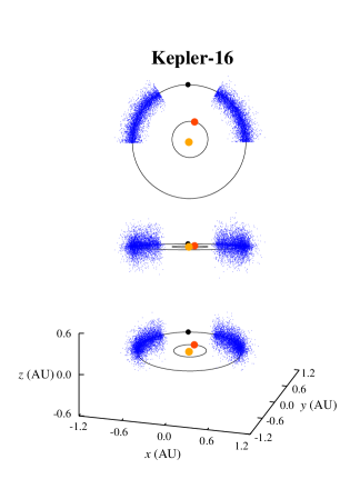
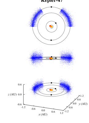
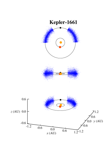
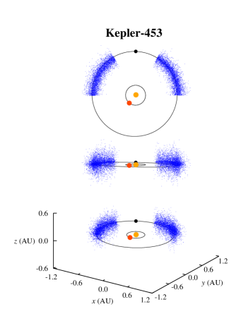
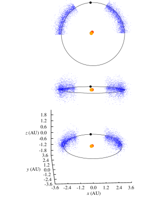
We randomly generated the initial semimajor axes of these objects using a Gaussian distribution with a range of around the semimajor axis of their corresponding CBPs. Their initial eccentricities were also randomly generated between 0 and using a one-sided Gaussian distribution with . Initial orbital inclinations were chosen from a range of 0 to and assigned at random following a one-sided Gaussian distribution with . The initial values of the arguments of periastron, longitudes of ascending node, and mean-anomalies of Trojan planets were chosen to follow a uniform distribution from to . The combination of these three angles were set to place Trojan objects between and on the either side of the planet. Figure 1 shows the spatial distribution of these bodies.
3 Dynamical Analysis
For each Trojan planet, we integrated the four-body system of binary-CBP-Trojan for 1 Myr (in Kepler-47, these integrations were carried out for the six-body system of binary-CBPs-Trojan). The time step of integrations were set to 1/30th the orbital period of the central binary. We stopped an integration when a Trojan planet collided with its host CBP or one of the binary stars. We also considered a Trojan to have been ejected from the system when its orbital period became equal to or larger than times the orbital period of its host CBP.
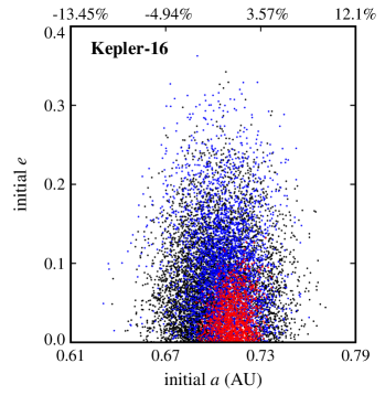
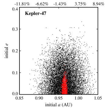
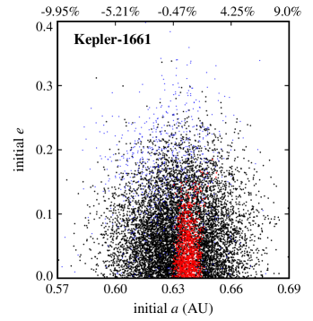
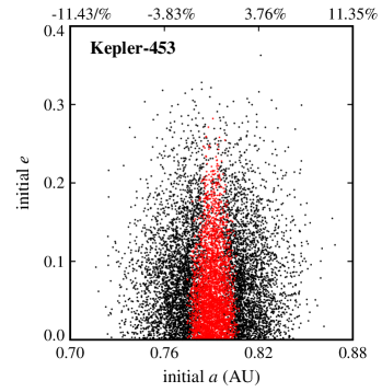
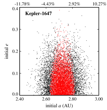
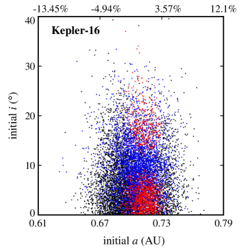
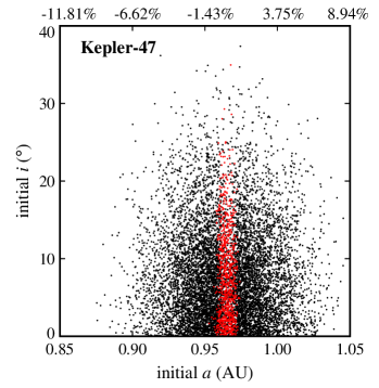
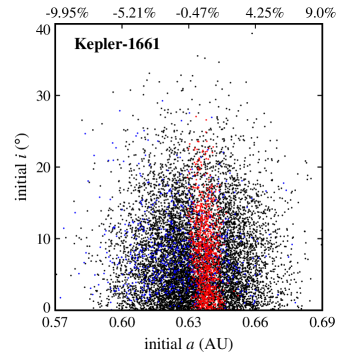
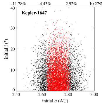
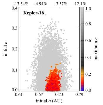
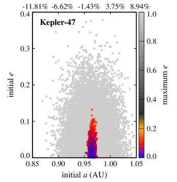
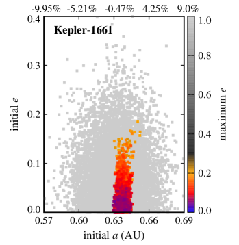
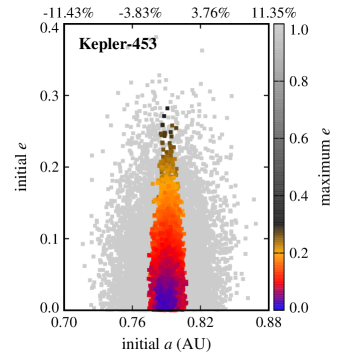
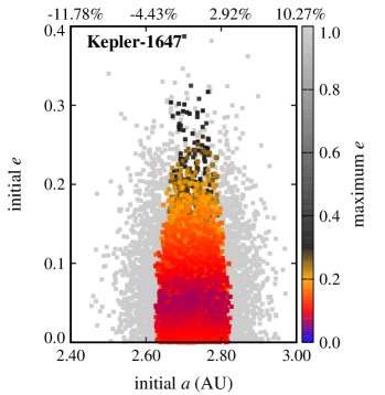
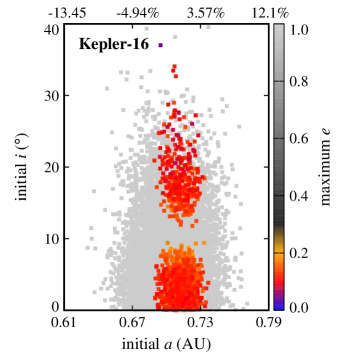
Figures 2 and 3 show the results. In these figures, the final dynamical state of each Trojan is shown in term of its initial semimajor axis , eccentricity , and orbital inclination . Points colored black represent Trojans that collided with their host CBP, blue corresponds to ejection from the system, and red indicates Trojans that remained in orbit for the duration of the integration. Table 4 shows the number of Trojan planets in each category.
As expected, collisions between a Trojan planet and one of the stars of the binary are rare (Table 4). That is due to the fact that when a planet enters the region of instability around the central binary, the perturbation of the two stars will increase its orbital eccentricity causing it to be ejected from the system instead of colliding with the binary stars.
Also, as expected, ejection is not a common outcome. That is because Trojan planets were initially distributed around the Lagrangian points of each CBP (that is, inside the CBP’s potential well) where they are strongly coupled to their host planet. The large number of ejections in the Kepler-16 and Kepler-1661 systems is, however, due to the close proximity of their CBPs to the inner unstable region of the host binaries. In these systems, slight perturbations from the binary increases the orbital eccentricities of Trojan planets (especially those with initially higher eccentricities) causing them to gradually enter the binary’s instability region where the gravitational effect of the binary scatters them to large distances. This can be seen in figures 2 and 3 where the stable region in Kepler-16 and Kepler-1661 systems are slightly off-centered toward larger semimajor axes.
As Table 4 shows, collision with the host CBP is the most common outcome. The reason is that the perturbation of the binary, and in the case of Kepler-47, that of the two inner planets, increases the orbital eccentricity of the Trojan body, gradually shifting its orbit into a collision course with its closest object, its host CBP (recall that integrations were carried out for individual four-body or six-body systems). It is, therefore, not surprising that Kepler-47c has the highest number of collisions, and Kepler-1661b is the second, as it has the smallest periastron distance compared to other HZ CBPs. The number of collisions drops considerably in the Kepler-1647 system where the CBP has the largest semimajor axis among all Kepler circumbinary systems.
One interesting result of our integrations is the final number of stable Trojan planets in each system. As shown in Table 4, except for Kepler-16b, the number of stable Trojans at the (leading) and (trailing) Lagrangian points of all other CBPs are statistically identical. However, in the Kepler-16 system, more Trojan planets are stable at than around . At the first glance, this seems to be in contrast to the number of Trojan asteroids at the Lagrangian points of Jupiter where more than 2/3 of these bodies are around the . However, it is important to note that a comparison between the Trojan planets considered here and Jupiter’s Trojan asteroids is not entirely valid. The planets considered here strongly affect the dynamics of their host CBP and must be considered within their full -body system whereas Trojan asteroids are effectively massless particles with no effects on the orbit of Jupiter. The dynamics of these bodies, in addition to their interaction with Jupiter, is also heavily affected by non-gravitational forces as well as their mutual collisions, two factors that do not exist in the our systems. We are currently investigating this asymmetry in Kepler-16 stable Trojans and will publish our results in a future article.
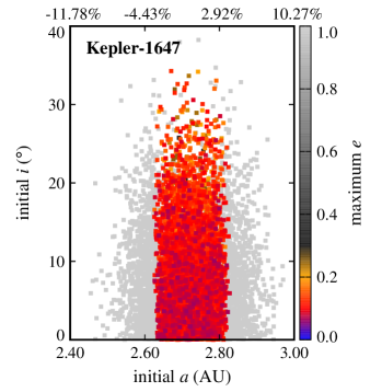
Another interesting result, as depicted by figures 2 and 3, is the extent of the region of stability. In systems where the CBP is close to the binary (Kepler-16, Kepler-1661) and where there are other strong perturbations (Kepler-47), stable Trojans are limited to a narrow region in semimajor axis and include only those with low eccentricities. However, in a system like Kepler-1647 where the CBP is farther out, the stability region expands both in semimajor axis and eccentricity.
Figure 3 also shows a gap in the stable region around Kepler-16b where, for a small range of inclination, the orbit of the Trojan planet becomes unstable. We speculate this island of instability to correspond to unstable inclination resonances between the Trojan planet and the central binary. Investigation on this topic is currently underway and will be published elsewhere.
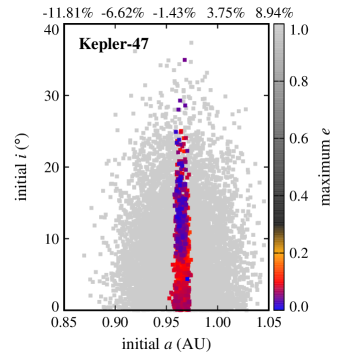
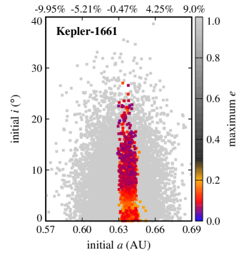
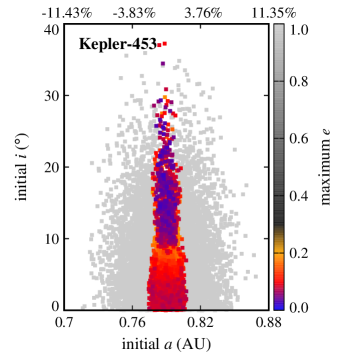
The extent of the stability region with regard to orbital eccentricity raises the question whether Trojans with higher eccentricities will be stable if integrations are continued for longer times (e.g., 10-100 Myr). While to answer this question, continuing integrations seems to be the natural choice, in practice, the short periods of the binaries considered here (periods vary from 7 days for Kepler-47 to 41 days for Kepler-16) combined with small time steps (1/30th of the period of the binary) make the extension of integrations to longer times prohibitive. For this reason, instead of direct integration, we used the value of the maximum eccentricity of each Trojan as a measure of its long-term stability. In general, the value of allows the identification and exclusion of regions of the parameter space where the orbit of an object becomes parabolic (unstable). The lower the value of , the longer the Trojan will maintain its orbit. Figures 4 and 5 show for all Trojans in our systems in terms of their initial eccentricities and orbital inclinations. As shown in these figures, the range of the semimajor axes of Trojans with the lowest varies between and of the range of the semimajor axes of their corresponding CBPs. In the next section, we consider Trojan planets within this range for calculating TTVs.
We would like to note that, because in different systems, transits occur at different times, a more appropriate way to compare the dynamical states of the systems would be to integrate them for the same number of transits rather than a fixed amount of time (e.g., 1 Myr). For instance, given that in the systems studied here, the orbital period of Kepler-1647b is almost three times the orbital periods of other CBPs, it is possible that if the four-body systems of binary-CBP-Trojan in Kepler-1647 were integrated for 3 Myr, more Trojans would become unstable and their region of stability would become smaller. We would, however, like to emphasize that the purpose of this paper is not to study the dynamical evolution of Kepler CBPs and their hypothetical Trojans. The goal of this paper is to assess the detectability of such Trojan bodies via the transit timing variation method. Stability analyses are merely carried out to exclude unstable systems from the TTV integrations.
4 Transit Timing Variations
To calculate the transit timing variations of a CBP due to the effect of a Trojan planet, the orbit of the CBP must be integrated while subject to the perturbation of the Trojan. Although, intrinsically, these integrations are similar to those carried out for the stability analyses, it is not possible to use the results of the stability integrations to calculate the TTVs. The reason is that TTV integrations require much smaller time steps to resolve the orbital interpolations necessary for calculating variations in the orbit of a CBP.
Before explaining the TTV integrations, we would like to note that it is unnecessary to carry out these integrations for a long time. Because the purpose is to calculate the amplitude of TTVs, an integration time to produce a few TTV cycles will suffice. Also at this stage, it is not necessary to carry out integrations for all stable Trojans. Many of these bodies are close to one another in the parameter-space and as a result, the amplitudes of the TTVs they produce will be close as well. A more efficient approach is to integrate only a sample of them.
To construct such a sample, we divided the population of stable Trojans in each system into 18 zones: three in radius from the central binary and six in angle from the CBP with three leading and three trailing the planet. We then randomly chose 300 Trojans from the 18 zones in each of the systems of Kepler-16, Kepler-453, and Kepler-1647, 200 from the system of Kepler-1661 and 100 from the Kepler-47 system. The smaller sample size in Kepler-1661 is the result of its smaller population of Trojans. In the case of Kepler-47, not only is the population smaller, but also the integrations take considerably more time.
We integrated the four-body system of Binary-CBP-Trojan (six-body in the case of Kepler-47) for each Trojan planet in the sample and for the duration of two complete TTV cycles with a time step of 0.001 days. This integration time translates to 36 transits at the low-end for Kepler-1647 and 280 transits at the high-end for Kepler-47. We assumed that at , the primary star was at the origin of coordinate system and placed the CBP on the -axis with the positive direction of the axis toward the observer. We determined the times of mid-transits of the CBP by interpolating between the times before and after its center crossed the line of sight to the center of the star.
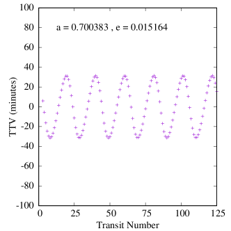
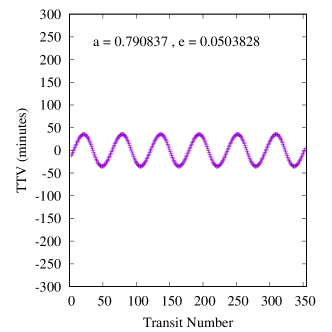
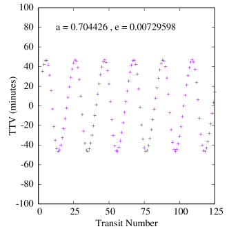
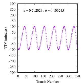
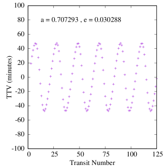
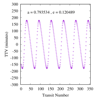
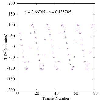
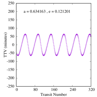
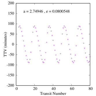
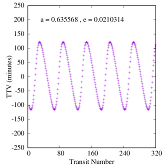
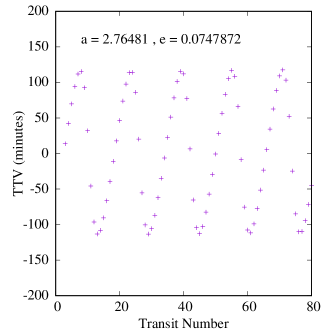
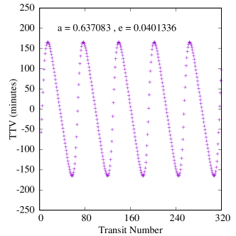
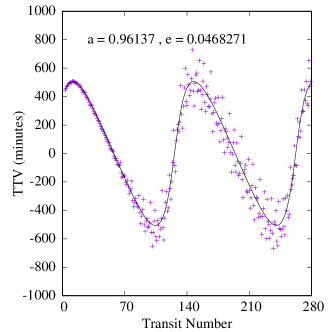
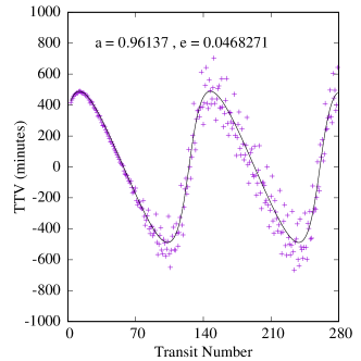
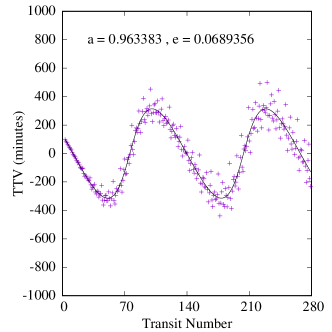
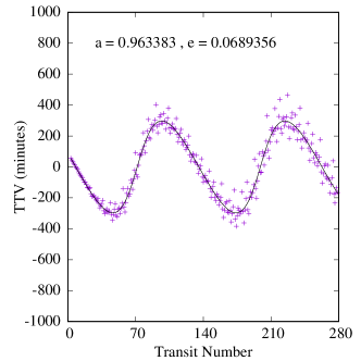
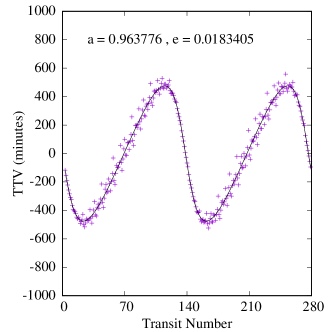
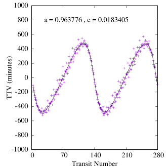
Figures 6-8 show samples of the results. Because the mass of the inner planet in the Kepler-47 system is not well constrained, we calculated two sets of TTVs for this system, one with the inner planet being 2.073 Earth-masses and one with its highest possible mass, 25.77 Earth-masses (Orosz et al., 2019). Also, because the variations in the orbit of Kepler-47c is due to the combined effects of the two inner planets and the Trojan body (it is not possible to separate these effects), we fit a tilted sine function to each TTV, and take the amplitude of the fitted function to be the amplitude of the TTV. We note that, as shown in figure 8, the effect of the mass of the inner planet on the transit timing variations of Kepler-47c is almost negligible.
Table 5 shows the maximum, minimum and the median amplitudes of the TTVs in all our systems, arranged in descending order of CBP mass. A few interesting features appear in this table and figures 6-8.
First, as shown by the figures, the amplitudes of TTVs increase with an increase in the range of eccentricities of the Trojan planet (within the stable region). This is an expected result because Trojans with larger eccentricities have closer approaches to their host CBPs which enhances the effect of their perturbations.
Second, Table 5 also shows that both the periods and amplitudes of the TTVs increase as the CBP mass becomes smaller. This is expected and consistent with the findings of Agol et al. (2005), Steffen & Agol (2005), and Steffen & Agol (2007) who showed that when the ratio of the mass of the perturber to the transiting planet increases, the amplitude of TTVs increase. In our study, the perturber is a planet with a fixed mass of one Earth-mass and, therefore, the ratio of its mass to the mass of the transiting planet (i.e., the CBP) increases as the mass of the CBP decreases.
Finally, a comparison between the amplitudes of TTVs in our systems and the transit timing variations of a large sample of Kepler planets (see figure 1 in Ford et al., 2011) indicates that the values of the TTVs of our systems fall squarely in the range of the sensitivity of the Kepler space telescope. That means, if Trojan planets can form and remain in stable orbits, Kepler data would provide the best resource to search for their TTV signatures. For instance, the period of secular oscillations of the TTVs of Kepler-16b is approximately 12.5 years, which suggests that the orbital characteristics of a massive Trojan planet could be inferred from a decade of transit data of this system.
5 Summary and Concluding Remarks
We have presented the results of a study of the detectability of Earth-mass Trojan planets as possible habitable bodies in the Kepler HZ circumbinary systems. We analysed the stability of these planets for different values of semimajor axis and eccentricity around the and Lagrangian points of their host CBPs, and identified regions of the parameter space where these planets can have long-term stable orbits. Results indicated that numerous stable orbits exist for Trojan planets in these systems. Motivated by the latter, we calculated the variations these Trojans planets create in the transit timings of their host planets and found that these TTVs fall squarely in the range of the timing precision obtained from the Kepler telescope’s long-cadence data. As expected, the prospect of detection is higher in systems where the CBP has a smaller mass and for stable Trojan planets with high eccentricities. As shown by Haghighipour et al. (2013), the results of our study can be used as a pathway to break the strong degeneracy associated with the RV-detection of Trojan planets around and (Giuppone et al., 2012) by combining the information obtained from the study of the transits of their systems and their TTVs.
Although the amplitude of the TTVs are within the range of photometric sensitivity of the Kepler telescope, if such TTVs are detected, it is not possible to determine if they are due exclusively to a Trojan planet. As shown by Nesvorný & Morbidelli (2008), Nesvorný (2009), Nesvorný & Beagué (2010), and Nesvorný et al. (2012), the mass and orbital elements of the perturbing body can be determined by analyzing TTVs alone in non-resonant systems. However, to determine these quantities in a near-resonance system, more information is needed. For instance, a catalog of TTVs, similar to those created by Haghighipour & Kirste (2011) can be used to determine the masses and orbital elements of the transiting and perturbing planets, although that approach too suffers from degeneracies. Another approach would be a combination of decade-long radial velocity and transit timing variation measurements (Laughlin & Chambers, 2002; Giuppone et al., 2012) along with high time resolution, -body integrations to identify non-contributing (i.e., unstable) regions of the parameter space.
The premise of our study is the assumption that planetary systems may exist in which planets are in a 1:1 MMR. Given the diversity of extrasolar planets, and, in particular, the existence of a variety of systems with different orbital resonances, it seems plausible that systems with Trojan or co-orbital planets may also exist. How such planetary systems form, however, is an important question that requires deep investigation. As mentioned in the introduction, the in-situ formation of 1:1 resonant planets is rather unlikely. Planet migration is also destructive and does not allow systems to maintain their Trojan or co-orbital orbits. That leaves only one scenario, capture in a 1:1 MMR. Whether capture occurs during the formation, as a result of planet-planet interaction, and/or because of planet migration is a topic beyond the scope of this paper and requires more thorough investigations.
As a final note, our -body integrations show no preference for Trojan objects sharing the argument of periapsis or the longitude of the ascending node with the transiting planet. Therefore, from a late-stage, dynamical perspective and barring any requirements set by the formation mechanisms for co-orbiting planets, the probability of detecting a double transit is the square of the probability of detecting the transit of either the planet or its Trojan companion. Since the probability of detecting any planet in transit is on the order of 1 in 100, only 1 in 10,000 systems with a Trojan planet large enough to be detected might be so well aligned as to exhibit a double transit. Given that only 13 circumbinary planetary systems have been discovered by the transit method, a double transit system would be an extraordinary find.
References
- Agol et al. (2005) Agol, E., Steffen, J., Sari, R. & Clarkson, W. 2005, MNRAS, 539, 567
- Agol & Steffen (2007) Agol, E. & Steffen, J. H. 2007, MNRAS, 374, 941
- Beaugé et al. (2007) Beaugé, C., Sàndor, Zs., Ėrdi, B. & Süli, À. 2007, A&A, 463, 359
- Chambers et al. (2002) Chambers, J. E., Quintana, E. V., Duncan, M. J. & Lissauer, J. J. 2002, AJ, 123, 2884
- Socia et al. (2020) Socia, Q. J., Welsh, W. F., Orosz, J. A., et a. 2020, AJ, 159, 94
- Cresswell & Nelson (2006) Cresswell, P. & Nelson, R. P. 2006, A&A, 450, 833
- Deitrick et al. (2015) Deitrick, R., Barnes, R., McArthur, B., Quinn, T. R., Luger, R., Antonsen, A. & Benedict, G. F. 2015, ApJ, 798, 46
- Demidova & Shevchenko (2018) Demidova, T. V. & Shevchenko, I. I. 2018, AstL., 44, 119
- Demidova (2018) Demidova, T. V. 2018, SoSyR, 52, 180
- Doyle, et al. (2011) Doyle, L. R., Carter, J. A., Fabrycky, D. C., et al. 2011, Science, 333, 1602
- Ford & Gaudi (2006) Ford, E. B.& Gaudi, B. S. 2006, ApJL, 652, L137
- Ford & Holman (2007) Ford, E. B. & Holman, M. J. 2007, ApJL, 664, L51
- Ford et al. (2011) Ford, E. B., Rowe, J, F., Fabrycky, D. C., et al. 2011, ApJS, 197, 2
- Giuppone et al. (2010) Giuppone, C. A., Beaugé, C., Michtchenko, T. A. & Ferraz-Mello, S. 2010, MNRAS, 407, 390
- Giuppone et al. (2012) Giuppone, C. A., Benítez-Llambay, P. & Beaugé, C. 2012, MNRAS, 421, 356
- Hadjidemetriou & Voyatzis (2011) Hadjidemetriou, J. D.& Voyatzis, G. 2011, CeMDA, 111, 179
- Haghighipour & Kirste (2011) Haghighipour N. & Kirste, S. 2011, CeMDA, 111, 267
- Haghighipour et al. (2013) Haghighipour, N., Capen, S. & Hinse T. C. 2011, CeMDA, 117, 75
- Heyl & Gladman (2007) Heyl J. S. & Gladman, B. J. 2007, MNRAS, 377, 1511
- Holman & Murray (2005) Holman, M. J. & Murray N. W. 2005, Science, 307, 1288
- Kostov et al. (2016) Kostov, V. B., Orosz, J. A., Welsh, W. F., et al. 2016, ApJ, 827, 86
- Laughlin & Chambers (2002) Laughlin, G. & Chambers, J. E. 2002, AJ, 124, 592
- Leleu et al. (2018) Leleu, A., Robutel, P. & Correia, A. C. M. 2018, CeMDA, 130, 24
- Leleu et al. (2019) Leleu, A., Coleman, G. A. L. & Ataiee, S. 2019, A&A, 631, A6
- Lyra et al. (2009) Lyra, W., Johansen, A., Klahr, H. & Piskunov, N. 2009, A&A, 493, 1125
- Marcy et al. (2001) Marcy, G. W., Butler, R. P., Fischer, D., et al. 2001, ApJ, 556, 296
- Miralda-Escude (2002) Miralda-Escude, J. 2002, ApJ, 564, 1019
- Nesvorný & Morbidelli (2008) Nesvorný, D. & Morbidelli, A. 2008, ApJ, 688, 636
- Nesvorný (2009) Nesvorný, D. 2009, ApJ, 701, 1116
- Nesvorný & Beagué (2010) Nesvorný, D. & Beagué, C. 2010, ApJL, 709, L44
- Nesvorný et al. (2012) Nesvorný, D., Kipping, D. M., Buchhave, L. A., Bakos, G. Á., Hartman, J. & Schmitt, A. R. 2012, Science, 336, 1133
- Orosz et al. (2019) Orosz, J. A., Welsh, W. F., Haghighipour, N., et al. 2019, AJ, 157, 174
- Penzlin et al. (2019) Penzlin, A. B. T., Ataiee, S. & Kley, W. 2019, A&A, 630, L1
- Quarles et al. (2012) Quarles, B., Musielak, Z. E. & Cuntz, M. 2012, ApJ, 750, 14
- Schwarz et al. (2015) Schwarz, R., Funk, B. & Bazsò, Á. 2015, Orig. Life Evol. Biosph., 45, 469
- Steffen & Agol (2005) Steffen, J. H. & Agol, E. 2005, MNRAS, 364, L96
- Steffen & Agol (2007) Steffen, J. H. & Agol, E. 2007, in: Transiting Extrasolar Planets Workshop ASP Conference Series, Eds. C. Afonso, D. Weldrake, & Th. Henning, 366, 158
- Veras et al. (2011) Veras, D., Ford, E. B., Payne, M. J. 2011, ApJ, 727, 74
- Welsh et al. (2015) Welsh, W. F., Orosz, J. A., Short, D. R., et al. 2015, ApJ, 809, 26

| Binary | Primary | Secondary | M.A. | |||||
|---|---|---|---|---|---|---|---|---|
| (AU) | (deg.) | (deg.) | (deg.) | (deg.) | ||||
| Kepler-16 | 0.6897 | 0.20255 | 0.22431 | 0.15944 | 0 | 263.464 | 0 | 188.888 |
| Kepler-47 | 0.957 | 0.342 | 0.08145 | 0.0288 | 0 | 226.3 | 0 | 310.8 |
| Kepler-453 | 0.944 | 0.1951 | 0.18539 | 0.0524 | 0 | 263.05 | 0 | 182.0931 |
| Kepler-1647 | 1.2207 | 0.9678 | 0.1276 | 0.1602 | 0 | 300.5442 | 0 | 90.62 |
| Kepler-1661 | 0.841 | 0.262 | 0.187 | 0.112 | 0 | 36.4 | 0 | 253.983 |
| Planet | Mass | M.A. | |||||
|---|---|---|---|---|---|---|---|
| (AU) | (deg.) | (deg.) | (deg.) | (deg.) | |||
| Kepler-16b | 106 | 0.7048 | 0.0069 | 0 | 318 | 0 | 148.507 |
| Kepler-47b | 2.073 | 0.2877 | 0.021 | 0.166 | 48.6 | 0 | 13.32 |
| Kepler-47c | 3.17 | 0.9638 | 0.044 | 1.38 | 306 | 0 | 165.4 |
| Kepler-47d | 19.03 | 0.6992 | 0.024 | 1.165 | 352 | 0 | 300.7 |
| Kepler-453b | 16 | 0.7903 | 0.0359 | 2.258 | 185.1 | 2.103 | 113.3028 |
| Kepler-1647b | 483.33 | 2.7205 | 0.0581 | 2.9855 | 155.0464 | -2.0393 | 301.37 |
| Kepler-1661b | 17 | 0.633 | 0.057 | 0.93 | 67.1 | 0.61 | 37.441 |
| Initial Population | Stable Population | |||||
|---|---|---|---|---|---|---|
| Kepler-16b | 4937 | 5063 | 356 | 765 | ||
| Kepler-47c | 4987 | 5013 | 484 | 412 | ||
| Kepler-453b | 5022 | 4978 | 1660 | 1719 | ||
| Kepler-1647b | 4944 | 4868 | 3002 | 3285 | ||
| Kepler-1661b | 4975 | 5025 | 520 | 501 | ||
| Planet | Collided with | Ejected | Collided with | Stable |
|---|---|---|---|---|
| Planet | Star | |||
| Kepler-16b | 5392 | 3291 | 16 | 1301 |
| Kepler-47b | 29 | 0 | 0 | - |
| Kepler-47c | 8921 | 0 | 0 | 896 |
| Kepler-47d | 154 | 0 | 0 | - |
| Kepler-453b | 6618 | 3 | 0 | 3379 |
| Kepler-1647b | 3523 | 2 | 0 | 6287 |
| Kepler-1661b | 8319 | 657 | 3 | 1021 |
| Planet | TTV Period | Maximum | Minimum | Median |
|---|---|---|---|---|
| (Transit #) | (min) | (min) | (min) | |
| Kepler-1647b | 16 | 194 | 10 | 97 |
| Kepler-16b | 20 | 151 | 4 | 71 |
| Kepler-1661b | 64 | 198 | 7 | 128 |
| Kepler-453b | 60 | 262 | 9 | 153 |
| Kepler-47c (High-mass) | 128 | 598 | 60 | 377 |
| Kepler-47c (Low-mass) | 128 | 598 | 60 | 390 |