On the Diameters of Friends-and-Strangers Graphs
Abstract.
Given simple graphs and on the same number of vertices, the friends-and-strangers graph has as its vertices all bijections from to , where two bijections are adjacent if and only if they differ on two adjacent elements of with images adjacent in . We study the diameters of connected components of friends-and-strangers graphs: the diameter of a component of corresponds to the largest number of swaps necessary to go from one configuration in the component to another. We show that any component of has diameter and that any component of has diameter, improvable to whenever is connected. These results address an open problem posed by Defant and Kravitz. Using an explicit construction, we show that there exist -vertex graphs and such that has a component with diameter. This answers a question raised by Alon, Defant, and Kravitz in the negative. As a corollary, we observe that for such and , the lazy random walk on this component of has mixing time. This result deviates from related classical theorems regarding rapidly mixing Markov chains and makes progress on another open problem of Alon, Defant, and Kravitz. We conclude with several suggestions for future research.
1. Introduction
1.1. Background and Motivation
Let and be -vertex simple graphs. Interpret the vertices of as positions, and the vertices of as people: say two people in the vertex set of are friends if they are adjacent and strangers if they are not. Each person picks a position to stand on, yielding a starting configuration. From here, at any point in time, two friends standing on adjacent positions may switch places: we call this operation a friendly swap. From the initial configuration, say the people have a final configuration in mind, and they know it can be reached from the initial configuration by some sequence of friendly swaps. What is the worst-case (over pairs of starting and final configurations) number of friendly swaps that is necessary in order for the people to achieve the final configuration from the starting configuration?
We may formalize the problem using the following definition.
Definition 1.1 ([DK21]).
Let and be simple graphs on vertices. The friends-and-strangers graph of and , denoted , is a graph with vertices consisting of all bijections from to , with bijections adjacent if and only if there exists an edge in such that
-
(1)
,
-
(2)
,
-
(3)
for all .
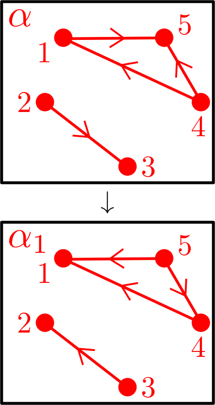
In other words, and differ precisely on two adjacent vertices of whose images under (and ) are adjacent in . For any such bijections , we say that is achieved from by an -friendly swap.

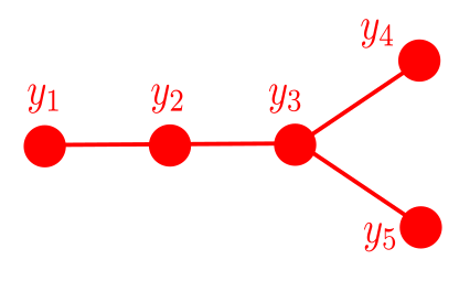
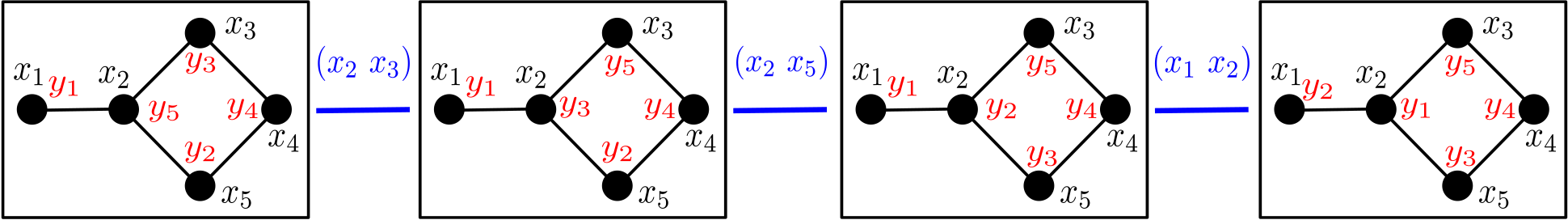
See Figure 1 for an illustration of Definition 1.1 on five-vertex graphs. Defant and Kravitz [DK21], in addition to introducing the framework of friends-and-strangers graphs, described the connected components of and in terms of the acyclic orientations of (the complement of ), and determined both necessary conditions and sufficient conditions for to be connected. In a different paper [Jeo22], we extend their results: [DK21, Corollary 4.14] states that is connected if and only if is a forest with trees of jointly coprime sizes, and we establish that if is biconnected (i.e., connected and with no cut vertex) and is a graph for which is connected, then is connected, settling [DK21, Conjecture 7.1]. In [Jeo22], we also initiate the study of the girth of friends-and-strangers graphs. Motivated by [KMS84] and connections to molecular programming as seen in [Bra+19], the framework of friends-and-strangers was later generalized by [Mil23] to permit for multiplicities onto vertices, in which many of the main results of [DK21, Wil74] were also generalized accordingly.
A central objective in the study of friends-and-strangers graphs is to determine necessary and sufficient conditions for their connectivity. Indeed, being connected corresponds exactly to the property that one can go between any two configurations in via some sequence of -friendly swaps. Of course, the conditions one may derive will depend upon the assumptions on and under which one works. If one elects to proceed under a regime in which cannot be connected (such as when and are both bipartite; see the discussion around [DK21, Proposition 2.7] and [ADK23, Subsection 2.3] for a parity obstruction which demonstrates why this is the case), one may instead study how small the number of connected components may be under this regime, and the natural question here is to ask for further conditions on and ensuring that achieves the smallest possible number of connected components. As pursued in [DK21, Sections 3 and 4] for (respectively) paths and cycles, one direction of inquiry is to fix (without loss of generality, as we will see in Proposition 2.3(1)) to be some particular graph, and study the structure of for arbitrary : see [Def+22, Lee22, WC23, Wil74, Zhu23]. It is also very natural to ask extremal and probabilistic questions concerning the connectivity of friends-and-strangers graphs, such as minimum degree conditions on and which ensure that is connected or for threshold probabilities on Erdős-Rényi random graphs regarding the connectivity of : see [ADK23, Ban22, Jeo23, Mil23, WLC23].
The setup proposed by Definition 1.1 is quite general. Indeed, friends-and-strangers graphs serve both as a common natural generalization of many classical combinatorial objects and as a framework which embodies many important problems in discrete mathematics and theoretical computer science. We illustrate this claim with a non-exhaustive listing of relevant examples. The graph is the Cayley graph of the symmetric group on the vertex set of generated by the transpositions corresponding to the edges of ; we refer the reader to [DK21] and the references therein for a comprehensive discussion regarding the relevance of friends-and-strangers graphs within algebraic combinatorics. Letting be the -by- grid and a star graph, studying is equivalent to studying the configurations and moves that can be performed on the famous -puzzle (with the central vertex of the star graph corresponding to the empty tile); see [BK23, DR18, Par15, Yan11] for similar inquiries of a recreational flavor. The works [Naa00, Sta08] both study the structure of the graph under certain restrictions on , while the works [BR99, Rei98] utilize to investigate the acyclic orientations of . Asking if and pack [BE78, KO09, SS78, Yap88, Yus07] in the graph packing literature is equivalent to asking if there exists an isolated vertex in . Studying the token swapping problem [Aic+22, Bin+23, BMR18, Mil+16, Yam+15] on the graph is equivalent to studying distances between configurations in . Finally, as we will briefly touch upon in Subsection 4.4, the interchange process on the graph [AF02, AK13, Ang03, BD06, CLR10, ES23, Ham15, HS21, Sch05] can be phrased in terms of (continuous-time) random walks on .
1.2. Main Results and Organization
Unlike the existing body of work that studies the connectivity of friends-and-strangers graphs, the present paper initiates the study of their diameters, corresponding to the length of the “longest shortest path,” with lengths of shortest paths evaluated over all pairs of vertices. Indeed, the diameter of a connected component of corresponds to the largest number of -friendly swaps necessary to achieve one configuration in the component from another. In a more recreational tone, if we think of as a generalized -puzzle, we are asking for the longest solution length for any solvable puzzle involving “board and rules .” The works [ADK23, DK21] both posed the following question, which asks whether the distance between any two configurations in is polynomial in the size of and .
Question 1.2 ([ADK23, DK21]).
Does there exist an absolute constant such that for all -vertex graphs and , every connected component of has diameter at most ?
In Section 2, we introduce some background that we shall need later in the work. Before tackling the more global Question 1.2, in Section 3, we fix (without loss of generality) to be a complete, path, or cycle graph, and derive upper bounds on the maximum diameter of a component of in each setting. Our results on paths and cycles address an open problem posed in [DK21, Subsection 7.3]. Furthermore, the discussion therein suggests that one must restrict their attention to rather contrived choices of graphs and in order for to have a component with diameter that is superpolynomial in the size of and , suggesting that Question 1.2 may be challenging to settle via constructive means if it holds in the negative.
In Section 4, we establish the main result of this article, Theorem 1.3, which answers Question 1.2 in the negative. We prove this theorem by constructing, for all integers , graphs and on the same number of vertices: see Figure 2 for a schematic diagram of the construction for . The construction is such that the number of vertices of and is , and there exist two configurations which lie in the same connected component of and for which the distance between and is .
Theorem 1.3.
For all , there exist -vertex graphs and such that has a connected component with diameter .
At the end of Section 4, we briefly discuss implications of Theorem 1.3 to the study of random walks on friends-and-strangers graphs, and deduce what might be thought of as the natural stochastic analogue of Theorem 1.3. Random walks on friends-and-strangers graphs model a variant of the interchange process where we may prohibit certain pairs of particles from swapping positions. This result contrasts many classical theorems regarding rapidly mixing Markov chains, all of which may be readily rewritten using the language of friends-and-strangers graphs, and makes progress on another open problem posed in [ADK23, Section 7]. We conclude the work with Section 5, which suggests several open problems and directions for future research.
1.3. Notation
In this article, unless stated otherwise, we assume that all graphs are simple. We employ standard asymptotic notation in this paper. Unless stated otherwise, all asymptotic notation in this paper will be with respect to . Purely for the sake of completeness, we state the following standard notation.
-
•
The vertex and edge sets of a graph are denoted by and , respectively.
-
•
The complement of the graph is denoted .
-
•
The statement that and are isomorphic is written as .
-
•
For a subset , we let denote the induced subgraph of with vertex set .
-
•
The open neighborhood of , which is the collection of all neighbors of , is denoted by . The closed neighborhood of is denoted . For a subset of vertices , we let
-
•
The disjoint of a collection of graphs , notated , is the graph with vertex set and edge set . This readily extends to expressing a graph as the disjoint union of its connected components.
-
•
The distance between is the length of the shortest path from to . The diameter of a component of is .
Graphs with vertex set that will be relevant later are
-
•
the complete graph , with ;
-
•
the complete bipartite graph , with , which naturally partitions into two sets (henceforth called partite sets);
-
•
the path graph , with ;
-
•
the cycle graph , with ;
-
•
the star graph .
2. Background
In this section, we introduce some background and summarize results from prior work that will be relevant later in the present paper, particularly in Section 3. Throughout this section and Section 3, we will assume that the vertex set of all graphs is , with edge sets as in Subsection 1.3. Note that if both and are , then the vertices of are the elements of , the symmetric group of degree .
2.1. Acyclic Orientations
An orientation of a graph is an assignment of a direction to every edge of , and an acyclic orientation of is an orientation with no directed cycles. Denote the set of all acyclic orientations of by . We will be interested in operations on acyclic orientations of called flips and double-flips, as defined in [DK21]. Notably, it was shown in [DK21, Theorem 4.7] that double-flips on acyclic orientations in are paramount in describing the connected components of .
Letting , converting a source of into a sink or a sink of into a source by reversing the directions of all its incident edges results in another acyclic orientation of . We call such an operation a flip, and we say that and are flip equivalent, denoted . In the literature, the equivalence classes in are called toric acyclic orientations; we refer the interested reader to [Che10, DMR16, MM11, Pre86, Spe09] for related reading. We will further say that we perform an inflip on if we convert a source into a sink (the direction of all incident edges “go into” the new sink), and an outflip if we convert a sink into a source.111In particular, we may apply these operations to isolated vertices.
Similarly, flipping a nonadjacent source and sink of into (respectively) a sink and a source results in another acyclic orientation of : we call such an operation a double-flip, and we say and are double-flip equivalent, denoted . It is easy to show that and are equivalence relations on . We denote the set of double-flip equivalence classes of by , and denote the double-flip equivalence class for which is a representative by .
Assume , and take . Associated to the acyclic orientation is a poset , where if and only if there exists a directed path from to in . We define a linear extension of to be any permutation such that whenever . We let denote the collection of linear extensions of . For any , it is not hard to see that there exists a unique acyclic orientation for which , and that this acyclic orientation is the result of directing each edge from to if and only if . It is also not hard to see that the poset associated to has a linear extension (e.g., for , we can construct a linear extension by setting to be a source of , then removing the source and all incident edges from ; in an abuse of notation,222We will commit similar abuses of notation in Section 3. They should not raise any confusion when invoked. we understand here as being mutated over the course of this greedy algorithm). We write
We refer the reader to [DK21, Section 4] for a more comprehensive discussion regarding why these notions are of importance in the study of friends-and-strangers graphs (though this is illuminated in passing in Subsection 2.2 and in the arguments of Section 3).
For a graph and acyclic orientation , we can partition the directed edges of any cycle subgraph of into and , corresponding to edges directed in one of two possible directions under in . The article [Pre86] studied precisely when an acyclic orientation could be reached from another by a sequence of inflips or outflips, while [Pro21] extends this result by providing an upper bound on the number of inflips or outflips necessary to reach from whenever .
Lemma 2.1 ([Pre86, Pro21]).
For , can be reached from by a sequence of inflips if and only if for every cycle subgraph of , . Furthermore, whenever this is the case, can be reached from by a sequence of at most inflips. Similarly, can be reached from by a sequence of outflips if and only if for every cycle subgraph of , . Furthermore, whenever this is the case, can be reached from by a sequence of at most outflips.
We build on Lemma 2.1. The following proposition establishes that we could have defined flip equivalence strictly with respect to inflips or outflips, as this would have resulted in the same notion.
Proposition 2.2.
Acyclic orientations are flip equivalent if and only if can be reached from by a sequence of inflips. Similarly, if and only if can be reached from by a sequence of outflips.
Proof.
The statement that is reachable from via a sequence of inflips (or outflips) implying is immediate. To prove the converse, notice that for any cycle subgraph of and acyclic orientations for which can be reached from by a flip, . Thus, if , then , so can be reached from via a sequence of inflips (or outflips). ∎
2.2. Background on Friends-and-Strangers Graphs
We mention those general properties of friends-and-strangers graphs that we will need later in the article. We refer the reader to [DK21, Section 2] for a thorough treatment of the general properties of friends-and-strangers graphs.
Proposition 2.3 ([DK21, Proposition 2.6]).
The following properties hold.
-
(1)
Definition 1.1 is symmetric with respect to and : we have that .
-
(2)
The graph is bipartite.
-
(3)
If or is disconnected, or if and are connected graphs on vertices and each have a cut vertex, then is disconnected.
The definitions concerning acyclic orientations that were introduced in Subsection 2.1 were observed in [DK21] to be central in describing the structure of the connected components of and , which are the graphs we will be interested in during Section 3. Specifically, we have the following theorems.
Theorem 2.4 ([DK21, Theorem 3.1]).
Let . Take any linear extension , and let denote the connected component of which contains . Then
and . In particular, is independent of the choice of .
Theorem 2.5 ([DK21, Theorem 4.7]).
Let . Take any linear extension , and let denote the connected component of which contains . Then
and . In particular, is independent of the choice of .
Defant and Kravitz [DK21] also determined precisely when is connected. The coprimality condition on the sizes of the components of in Theorem 2.6 may seem surprising at first glance. We refer the reader to the discussion around [DK21, Corollary 4.12] and [DK21, Corollary 4.14] to see where this condition emerges and why it is a natural one.
Theorem 2.6 ([DK21, Corollary 4.14]).
Let be a graph on vertices. Then is connected if and only if is a forest with trees such that .
3. Diameters of with One Graph Fixed
Before investigating (and settling) the more global question of whether or not the diameters of connected components of friends-and-strangers graphs are polynomially bounded (in the sense posed by Question 1.2), we begin by restricting our study by choosing one of the two graphs and to come from a natural family of graphs, and then establish bounds on the diameter of any connected component of .
3.1. Complete Graphs
We begin by setting . Take any two configurations that lie in the same connected component. Consider the following iterative algorithm, applied starting from and proceeding sequentially on . In an abuse of notation, is understood to be mutated over the course of this algorithm as we perform -friendly swaps to modify its mappings.
-
(1)
If , do nothing.
-
(2)
If , swap onto along a simple path, then swap back along the simple path that traversed.
It is straightforward to prove via induction that at the beginning of any iteration , and lie upon the same connected component of (so that the algorithm may always proceed), and that for all . Thus, when the algorithm terminates after iterations (it must be that at the beginning of the th iteration). For any iteration , step (2) requires at most -friendly swaps to move onto , and at most -friendly swaps to move back. This establishes that the diameter of any component of is therefore at most .
Finding the exact distance between two configurations in is known as the token swapping problem on in the theoretical computer science literature. The bound on the diameter of any component of is well known, and we also have a bound of on the diameter of any component of for particular choices of (e.g., see Remark 3.4). In general, computing exact distances between two configurations in , as well as the diameters of its connected components, is challenging, even when imposing additional assumptions on (e.g., see [Bin+23, Yam+15]). There do exist, however, exact polynomial-time algorithms which solve the token swapping problem for a number of choices of , including cliques [Cay49], paths [Jer85], stars [PV90], cycles [KSY19, van+16], and complete bipartite graphs [Yam+15]. See Subsection 5.5 for additional discussion regarding matters of hardness and approximation.
3.2. Path Graphs
In this subsection, we fix . We begin by introducing a notion which will serve as a monovariant in the proof of Proposition 3.2.
Definition 3.1.
For , call the ordered pair (, ) a -inversion if either
-
(1)
and ,
-
(2)
and .
Denote the number of -inversions by .
In other words, the ordered pair is a -inversion if the relative ordering of the inverse images of under is opposite that of . If (without loss of generality) is the identity permutation, then , the number of inversions of . It also follows immediately that if and only if .
Proposition 3.2.
Take , and let denote the corresponding connected component of . Let be the poset on for which if and only if there exists a directed path from to in under . Then , where denotes the number of comparable ordered pairs with , in .
Proof.
We will show for any that . Any -friendly swap reduces the number of -inversions by at most one, so . Now consider the following variant of the bubble sort algorithm, which we perform beginning from . Say , and swap down to position , yielding with . Now, say (with ), and swap down to position , yielding with for ; continue until we achieve . It is immediate that the execution of any swap performed during this algorithm would decrement by . Furthermore, any proposed swap in this algorithm can be executed, i.e., involves two elements which comprise an edge in . Indeed, Theorem 2.4 yields , but the existence of a swap in this algorithm that cannot be executed would yield (if the proposed swap fails to be an edge in , it is an edge in , and would be directed in opposite directions under and because the two elements comprising the swap constitute a -inversion), which is a contradiction. Thus, . If , it follows from that and , so is not a -inversion. Thus, , and therefore . ∎
Certainly, the two vertices incident to an edge of are comparable in the poset for any . This yields the following statement, as . For simplicity, we appeal to Theorem 3.3, rather than Proposition 3.2, in forthcoming arguments.
Theorem 3.3.
The diameter of any connected component of is at most .
Remark 3.4.
It is not hard to see that is connected (e.g., for any two configurations , the algorithm from Subsection 3.1 yields a path between and ). From the proof of Proposition 3.2, we have for any that , and when is the “reverse” of (i.e., for all ). So . Combined with Proposition 3.2, this establishes that the maximum diameter of a component of is , and thus . Thus, there exist families of -vertex graphs for which the maximum diameter of a component of has diameter . The same can be said for . ∎
Remark 3.5.
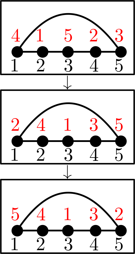
The upper bound of on in Theorem 3.2 corresponds to the number of ordered pairs (; ) that are incomparable in the poset . It follows from the proof of Proposition 3.2 that for arbitrary , any -inversion must be a pair of incomparable elements in , and . We now apply these observations to show that the upper bound on fails to be sharp: Figure 3 provides an illustration of our construction. For , consider the graph shown in Figure 3a, whose complement is shown in Figure 3b. We will take to be an acyclic orientation for which the edges in this connected component are oriented as in Figure 3c.


Assume (towards a contradiction) that there exist for which , so that all pairs of incomparable elements in are -inversions. Any two elements in are incomparable in , so the relative ordering of in must be the relative ordering of in reversed. Without loss of generality, assume has relative ordering , so has . Since , the element follows vertex in both and , so is not a -inversion. But is incomparable in , a contradiction. ∎
3.3. Cycle Graphs
In this subsection, we fix . The setting has been studied in the context of circular permutations [Kim16, van+16]. In particular, [Kim16, Procedure 3.6] provides an algorithm that achieves the minimal number of -friendly swaps between any two permutations in . Extracting these results yields that the diameter of is . In the spirit of Remark 3.4, it follows that there exist families of -vertex graphs for which has diameter , and it is worth asking what conditions on yield that the maximum diameter of a connected component of is at most quadratic in . In this direction, we have the following proposition.
Proposition 3.6.
If has an isolated vertex or , then the diameter of any connected component of is at most .
Proof.
Consider any which lie in the same component. If has an isolated vertex , then it must be that remains fixed over any sequence of -friendly swaps from to . Thus, it must be that any path from to in is a path in
from which the result follows from Theorem 3.3. For the setting , we will show that any in the same connected component will remain in the same component after removing some edge from , from which the desired result again follows immediately from Theorem 3.3. Assume (towards a contradiction) that every path from to in involves a swap over every edge in . Consider a shortest path from or , which has that and , and by the assumption. Consider the subsequence consisting of the first -friendly swaps of . This must be a shortest path from to in , and swaps upon at most edges of : say is an edge upon which a swap does not occur, and let be with this edge removed. Then is a shortest path from to in with length . This contradicts Theorem 3.3, which yields . ∎
We were unable to extend the bound from Proposition 3.6 to general , although we suspect that this is the truth (see Subsection 5.2). However, the existence of a universal constant such that the maximum diameter of a component of is remains highly desirable. In conjunction with Theorem 2.6, the following theorem yields such a result whenever is connected.
Theorem 3.7.
Let be a graph on vertices, and let denote the sizes of the components of . If , then any component of has diameter at most .
Proof.
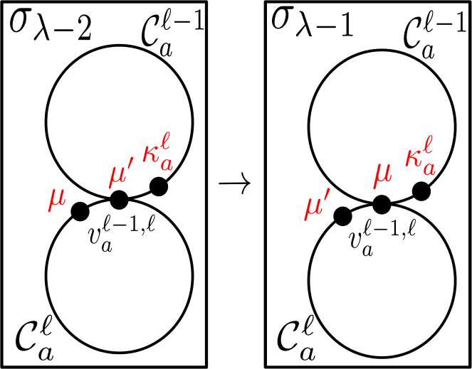
Certainly, . Without loss of generality, we assume that , and we denote the corresponding components of by , respectively. For , we let denote the acyclic orientation induced by on . We now fix such that . Before studying distances in , we will first bound the number of double-flips necessary to reach from . Certainly, for all , and by Proposition 2.2, we can reach in no more than inflips or outflips from . Observe that for any , we may return to by applying a different sequence of inflips; see Figure 4 for an illustration. Indeed, take a linear extension , labeled , and perform an inflip on by converting the source into a sink, so that is a linear extension of the poset associated to the resulting acyclic orientation in . Performing inflips on in this manner returns as a linear extension of the poset associated to the resulting acyclic orientation: since there exists a unique acyclic orientation for which , this acyclic orientation must be . Similarly, we can return to by applying a sequence of outflips.

Recalling that a double-flip applied to an acyclic orientation involves flipping a nonadjacent source and sink into (respectively) a sink and source, we thus proceed as follows. Starting from the acyclic orientation , perform a sequence of double-flips that act as inflips on sources in and outflips on sinks in until we have reached at least once. Specifically, begin by performing inflips on and outflips on until we either reach (at which point we begin performing outflips on sinks in ) or (at which point we begin performing inflips on sources in as described previously to return to every inflips). If we reach prior to , then perform outflips on sinks in (returning to every outflips) until is reached: from here, pair these outflips on sinks with inflips on sources in until we retain . Otherwise, we reach prior to , for which will be “offset” once we have , since we are performing inflips on sources which return to every inflips. In either case, call the resulting acyclic orientation , which satisfies for all while differs from by some offset . By tracing the preceding description and recalling Proposition 2.2, it follows that the number of double-flips we perform to reach from is bounded above by
By Bézout’s Lemma (recall that ), there exist integers such that
Thus, from , we can reach by performing outflips on for (returning to every outflips), while performing inflips on as discussed to reach . The number of double-flips we perform to reach from is therefore bounded above by
so at most double-flips are necessary to reach from .
We now turn to bounding for configurations in the same connected component. By Theorem 2.5, we have that for some . Denote and . By the preceding discussion, we can reach from in double-flips, yielding a sequence of acyclic orientations in the equivalence class with and . From , we will now construct a sequence of -friendly swaps which we can apply on ; see Figure 5 for an illustration. If the double-flip we performed to reach from inflips the source and outflips the sink in , it follows from that for any , . Indeed, if we had that , being a source in would imply that this edge is directed from to in , contradicting . Similarly, for any , . Thus, we can swap to and to in no more than -friendly swaps: it is easy to check that the resulting configuration remains in . Then we perform a -friendly swap which swaps and along the edge ( by the definition of a double-flip, so ). It is also straightforward to check that the configuration resulting from this interchange is now in .
Proceed similarly through all double-flips, and call the resulting configuration : this configuration satisfies . Since , it follows from Theorem 2.4 that lie in the same component of (specifically, the copy of in resulting from excluding the edge ). By Theorem 3.3, we can now reach from by performing no more than -friendly swaps. Altogether, we have that
so at most -friendly swaps are necessary to reach from . ∎
Corollary 3.8.
For , if is connected, .
Theorem 3.7 can now be invoked to establish the following general bound on the diameter of any connected component of , where is arbitrary. This proves that, in the sense of Question 1.2, the diameter of is polynomially bounded.
Theorem 3.9.
The diameter of any component of is at most .
Proof.
Consider two configurations in the same connected component. We construct an -vertex graph by adding a vertex to that is adjacent to all vertices in , so has a spanning star subgraph with central vertex . Define bijections by
The configurations are in the same component of . Indeed, from a sequence of -friendly swaps from to of shortest length, we can construct a sequence of -friendly swaps from to by replacing every swap in which occurs along by a sequence of three swaps along the following edges in :
It is straightforward to confirm that is a path from to , constructed from by “crossing” the vertex as needed. Since has a spanning star subgraph, has an isolated vertex, so it follows immediately that the components of have jointly coprime size. So by Theorem 3.7,
where . Let be a sequence of swaps from to of length at most . We construct from by removing all -friendly swaps involving : it is straightforward to notice that yields a path of length at most from to some cyclic rotation of , i.e., . Towards a contradiction, assume , and let be vertices along a shortest path from to satisfying for all . Such vertices exist due to our assumption on . By appealing to the same argument as above, we deduce that there exist cyclic rotations of such that for all . Since there exist distinct rotations of , the pigeonhole principle yields the existence of for which
for some rotation of , which is a contradiction. Therefore, we conclude that
The desired result now follows immediately. ∎
Corollary 3.10.
If satisfy , then we can reach from in no more than double-flips.
Proof.
Given an -vertex graph and satisfying , extract linear extensions , , and consider and as vertices of . By Theorem 3.9, , so let be a shortest sequence of swaps from to , so . Let be the subsequence of consisting of all indices for which is reached from by a -friendly swap across the edge . Since is smallest possible, two consecutive swaps of cannot both be across the edge , so . We will now describe how to use to construct a sequence of acyclic orientations, with and , for which is reachable from by a double-flip for all . The desired result will then follow immediately.
Since we reached from by swapping along the graph (specifically, the copy of in resulting from excluding the edge ), it follows from Theorem 2.4 that . Let be the result of taking and performing a double-flip which involves an inflip on the source and an outflip on the sink . Note that (we swapped these two vertices to reach from ), so , from which it follows that this is a valid double-flip.333This correspondence between double-flips and paths in is the same as that which was observed in the first paragraph of the proof of [DK21, Theorem 4.1]. It is easy to check that , and by appealing to Theorem 2.4 as before, . Continuing like this sequentially on (the preceding discussion being the case) yields the desired sequence : for the case , it follows as before from Theorem 2.4 that and are linear extensions of the poset (i.e., associated to the same acyclic orientation of ), so the final acyclic orientation in is . ∎
4. Proof of Main Result
4.1. The Graphs and
We begin with the following observation. One can understand this as the central vertex of acting as a “knob” rotating around , and all other vertices of moving cyclically around it: such swaps in the same direction are needed for all vertices of to return to their original positions in the starting configuration. This interpretation will help motivate our construction.
Lemma 4.1.
Every connected component of is isomorphic to .
Proof.
Consider a component of with permutation such that is the central vertex of . With , construct by defining to be the permutation achieved by starting from and swapping rightward times (e.g., ). It follows that is a graph isomorphism. ∎
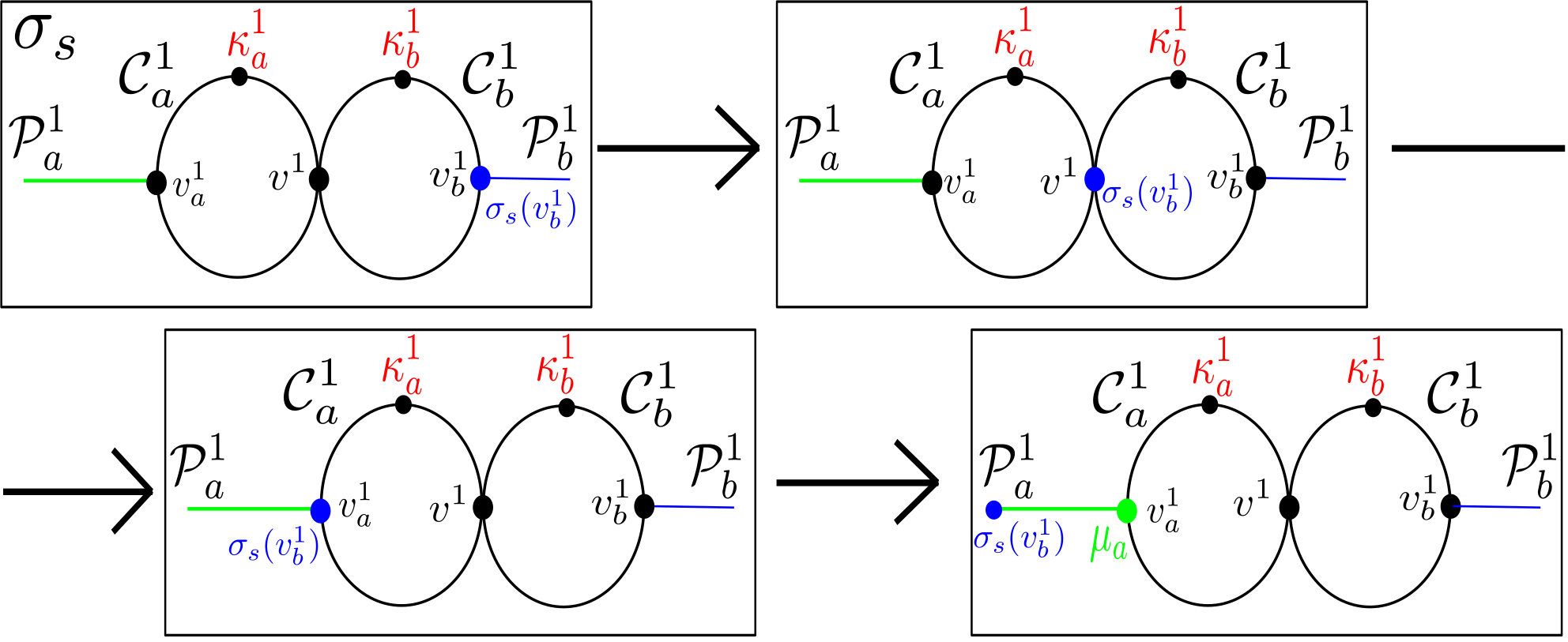
We will now construct the graphs and , for every integer , that we study to prove Theorem 1.3. In the following description, assume we have fixed some arbitrary integer .
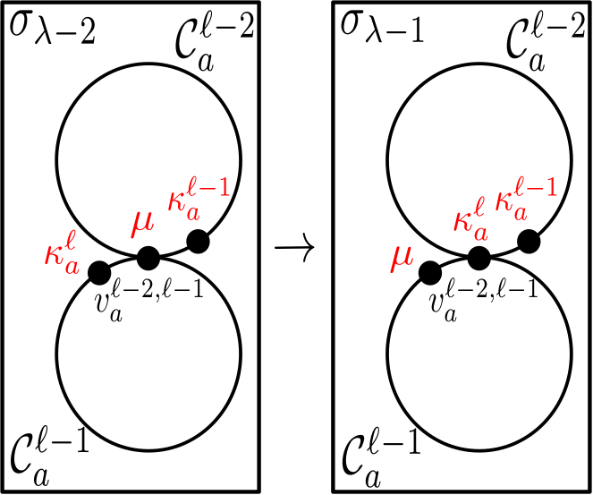
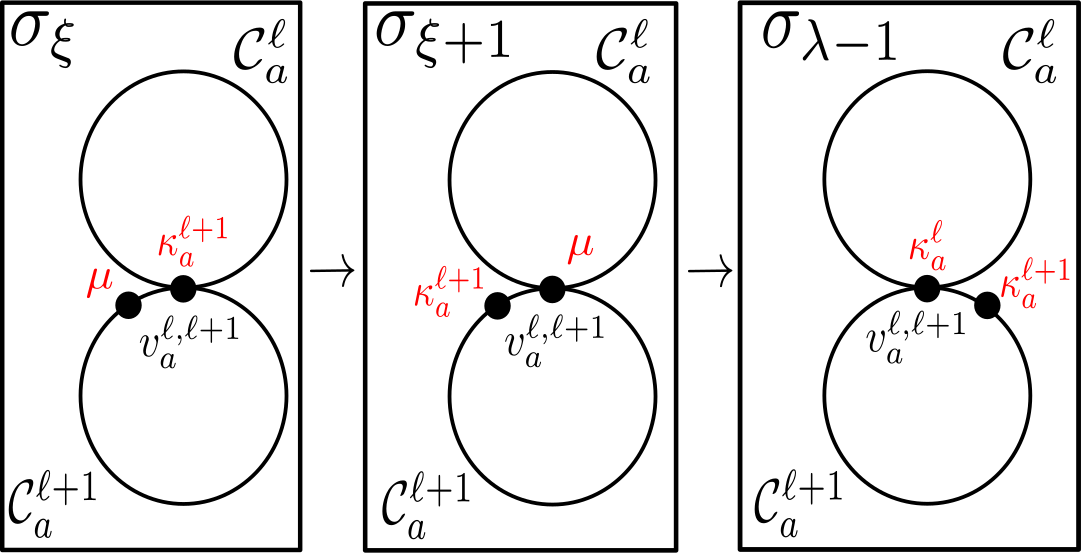
The Graph .
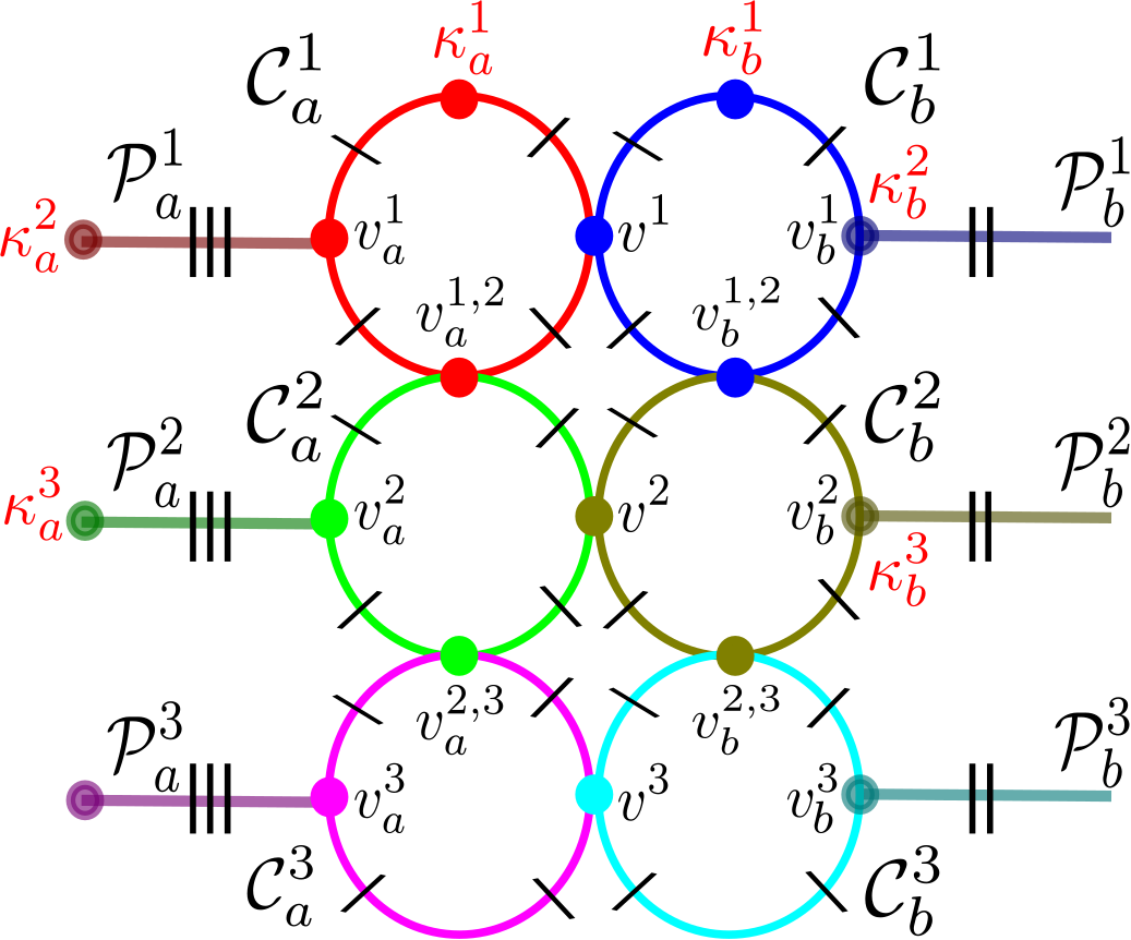
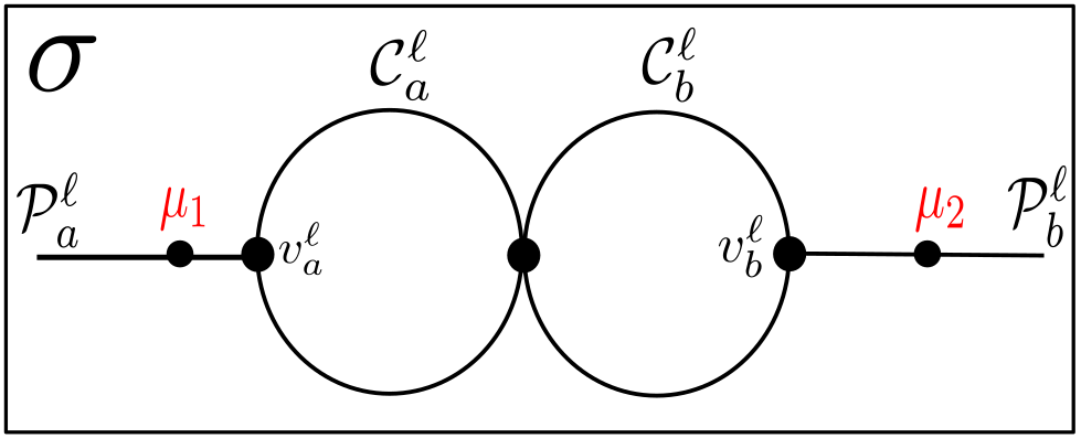
The graph contains an array of cycle subgraphs, with adjacent cycles intersecting in exactly one vertex. Say has layers, indexed by ; we will subscript subgraphs and vertices corresponding to the “left column” of by , and those in the right by . As such, we denote the left and right cycle subgraphs in layer by and , respectively. Corresponding to each and is a path subgraph of extending out of it; that corresponding to is denoted , and similarly for . Denote the subgraph of consisting of the th layer by . The subgraph consisting of and is denoted , and similarly for and . Denote, whenever they are defined for ,
For each of the following sets, we place three inner vertices in the path in between the two vertices in the set:
The analogous statement for holds. The exceptions are layers and : we place seven inner vertices in the upper path from to in and the upper path from to in , and seven inner vertices in the lower path from to in and from to in . It follows from our construction that for every ,
We will also set,444It will be important that, for every , has exactly one more vertex than . The choice of the lengths of these paths, as well as the number of inner vertices in the segments of the cycle subgraphs, is not terribly important as long as they are not too small. The values we chose here suffice. for every ,
so that the graph has
vertices. (Indeed, it can be checked that layer has vertices, and for each subsequent layer, we add new vertices to the graph .) Figure 6 illustrates this construction for .
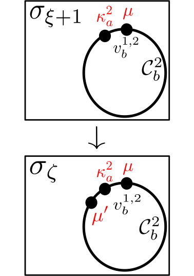
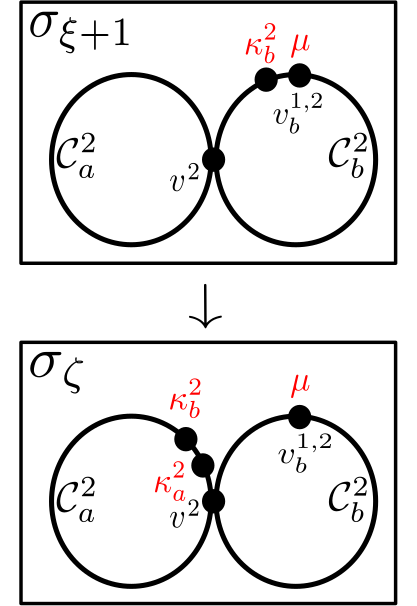
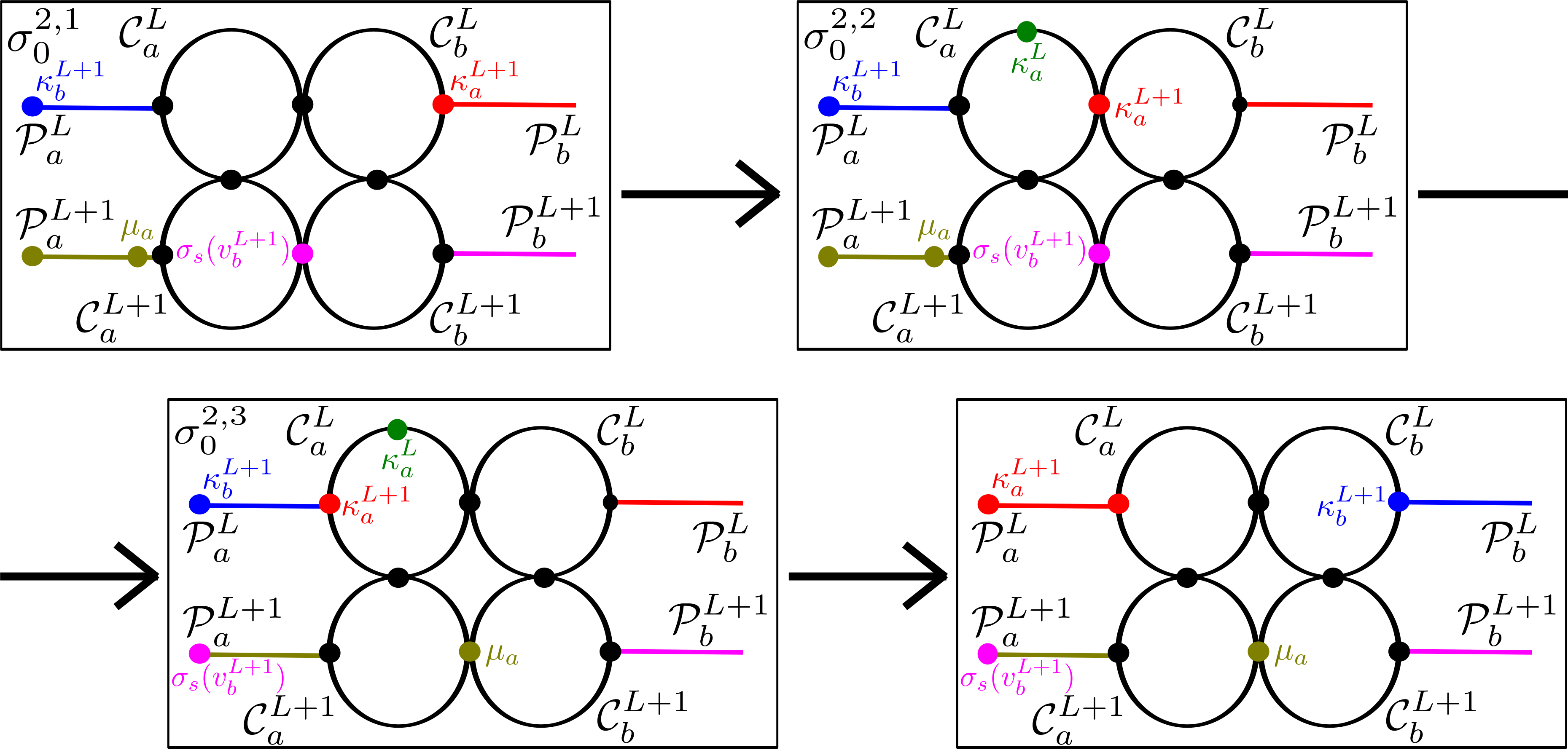
The Graph .
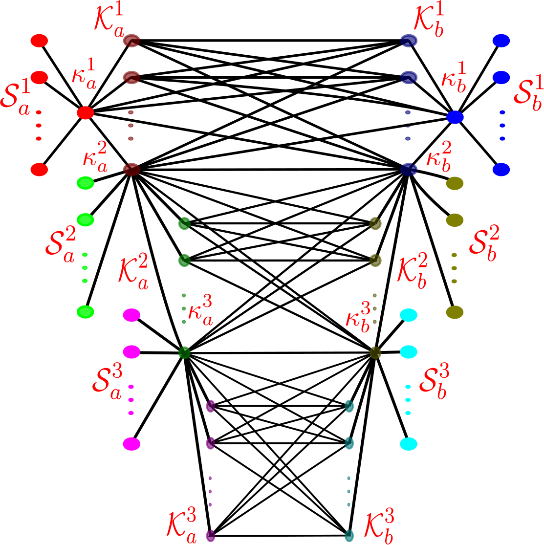
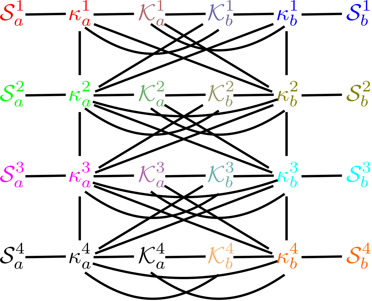
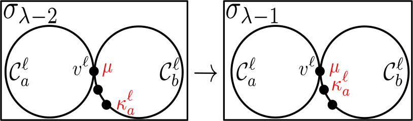
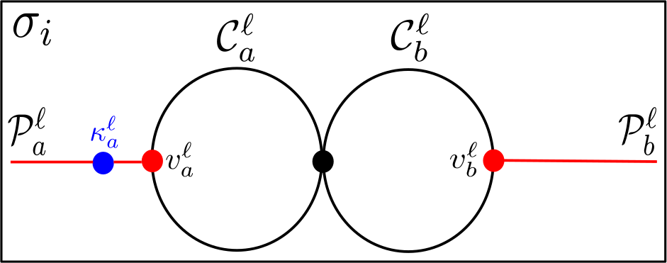
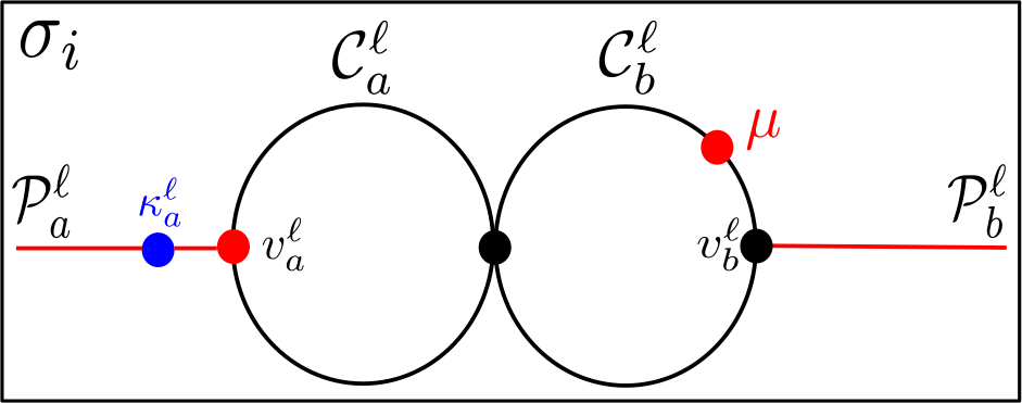
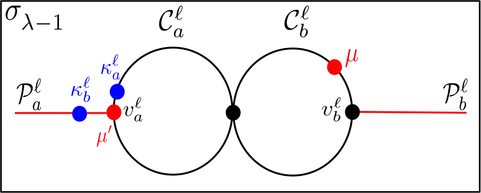
We construct a complementary graph for each : we assign to each cycle subgraph and of a corresponding “knob vertex” in , denoted and , respectively; we set a collection of vertices of to swap only with each knob. The construction of proceeds sequentially according to . Take two disjoint copies of , denoted and , with central vertices and , respectively, and a complete bipartite graph with vertices in each of its partite sets and . Set and adjacent to all the vertices in . If , this completes the construction of . If , take one vertex each in and , which shall correspond to and , central vertices of star subgraphs (again both isomorphic to ) and , respectively, and also construct complete bipartite graph with vertices in each of its partite sets and . Set and adjacent to all the vertices in . Proceed similarly: for , take two vertices of in opposite partite sets and construct , , and , related as before, until all vertices are exhausted. We shall often refer to vertices and as knob vertices of . Figure 7 illustrates this construction for , while Figure 8 provides a “collapsed” view of our construction.
The Starting Configuration and its Connected Component .
Take an arbitrary and graphs , . We are now going to describe a specific starting configuration which lies in the connected component of ; we will later show that there exists a different configuration in whose distance from is . Henceforth, we abbreviate and to and . In forthcoming discussions, and will be understood to be arbitrary such graphs on the same number of vertices.
Take all vertices in and place them onto , and the vertices in onto ; if , we place onto the leftmost vertex of and onto . Now take subgraph of : place onto the middle vertex of the upper path between and (which has seven vertices), and place all leaves of onto the remaining vertices of in some way. Similarly, take : place onto the middle vertex of the upper path between and , and place all leaves of onto the remaining vertices of . This has filled all mappings on the subgraph of by vertices in , , and , and thus yields if .
Proceed sequentially according to the layer : say we placed all vertices of , , and for onto the corresponding of . Place all vertices in onto , and the vertices in onto ; if , place onto the leftmost vertex of and onto . Now take , and place its leaves onto the remaining vertices in . Similarly take , and place its leaves onto the remaining vertices in . An illustration of this starting configuration is given in Figures 6 and 7: the vertices of a particular color in Figure 7 are placed upon the correspondingly colored subgraph in Figure 6 to achieve .
Remark 4.2.
By the construction of , for any ,
As such, all leaves of a star subgraph or of are placed onto a corresponding cycle subgraph or of , respectively. This yields that, for any ,
In other words, the number of vertices upon any cycle subgraph or of which are not leaves of the corresponding star subgraph of , under , is exactly two. ∎
We introduce the following definition for notational convenience in forthcoming arguments.
Definition 4.3.
Fix .
-
•
The boundary of is the subset of defined for .
-
•
The boundary of is the subset of defined for .
In Subsections 4.2 and 4.3, unless otherwise stated, we fix an arbitrary integer and refer to the graphs and , with denoting the corresponding starting configuration. We elect to refer to paths in as swap sequences, which are denoted by the vertices and edges in that constitute the path. More specifically, a swap sequence of length is a sequence of vertices for which for all .
4.2. Configurations in
In this subsection, we derive properties satisfied by all vertices in . Intuitively, our aim in this subsection is to uncover many conditions satisfied by all of the vertices in , which has the effect of producing strong rigidities on the corresponding swapping problem. These rigidities will allow us to argue in Subsection 4.3 that in order to move certain vertices in down and across the graph , we necessarily must perform very specific sequences of swaps.
Remark 4.2 observes that in the starting configuration , the leaves of any star graph or lie upon the vertices of and , respectively. In particular, for any cycle subgraph in , exactly two vertices that are not leaves of lie upon them; an analogous statement holds for cycle subgraphs of the form . We begin our study of by establishing that this property is maintained after any sequence of swaps in beginning at , i.e., that all vertices in satisfy this property: we prove this in Proposition 4.4.
Proposition 4.4.
Any satisfies, for all ,
Remark 4.5.
Although Proposition 4.4 describes a global property maintained by all configurations in , we frequently appeal to it (for sake of brevity) as a local property satisfied by specific configurations in during the proof of Proposition 4.4.555Making this clarification is important, as the proof proceeds by assuming (towards a contradiction) that Proposition 4.4 is satisfied by particular configurations in and is violated by another. This practice of localizing a more global statement to a particular configuration will also be utilized for other results in later proofs in this section, and it should not raise any ambiguity whenever it is invoked. ∎
Proof of Proposition 4.4.
Assume (towards a contradiction) that the proposition is false, so there exists a swap sequence with in of shortest length containing a vertex violating Proposition 4.4: violates Proposition 4.4, while all for satisfy it, and . Thus, there exists a star subgraph (of form or ) of and a leaf such that is in the appropriate cycle subgraph, but is not. Say for : raising a contradiction when is entirely analogous. Here, has and , , so and is reached from by swapping and . Figure 9 depicts the configurations described in the following two cases.
Case 1: .
Case 2: .
Here, , and
Proceeding backwards in , it must be that either
note that , since . Indeed, if not, swapping and directly from raises a contradiction on being minimal. Now, implies
since if both preimages differ, . Thus, and
by Proposition 4.4 (on ), so is not a leaf (see ). We further assume that
raising a contradiction for the cases and can be done analogously. So
Altogether, we have that
and since and , . Thus, violates Proposition 4.4, contradicting being minimal.
∎
Proposition 4.4 restricts the preimages of the leaves of and under any . We now derive a restriction on the preimages of all other vertices in under any . As Proposition 4.6 formalizes, for such , any vertex in is close to its preimage in .
Proposition 4.6.
Any configuration must satisfy the following four properties.
-
(1)
The layer knob vertices lie upon the corresponding subgraph of , i.e.,
-
(2)
For , the layer knob vertices lie upon the subgraphs or , i.e.,
-
(3)
For , any vertex in that is not a layer knob lies upon , i.e.,
and every vertex in lies upon , i.e.,
-
(4)
For , there is at most one not in , i.e.,
Confirming that the starting configuration satisfies these four properties is straightforward. Case 4 of the proof of Proposition 4.6 relies on the following Lemma 4.7, which is illustrated in Figure 10. In the statement of the lemma, we elect to index the final term of the swap sequence by as this is where the result applies in the proof of Proposition 4.6.
Lemma 4.7.
Let with , be a swap sequence in such that for all , satisfies the four properties of Proposition 4.6. Then for all and , the following two statements hold.
-
(1)
If , then
-
(2)
If , then
Proof of Lemma 4.7.
Fix to be a swap sequence satisfying the assumptions of Lemma 4.7. We prove the two statements of Lemma 4.7 hold for all inductively for . They can be checked to hold for all when , so assume they are true for some . We prove that satisfies both statements for all . In what follows, assume we refer (unless stated otherwise) to some fixed, arbitrary . We break into cases based on whether or not .
Case 1: .
We will further break into subcases based on whether or not .
Subcase 1.1: .
By the induction hypothesis, we have that
| (4.2) |
If and , then satisfies Lemma 4.7(1) since
and satisfies Lemma 4.7(2) trivially.666Generally, in what follows, we do not comment on the “other statement” in Lemma 4.7 holding trivially, and only check the statement which applies, depending on whether or not in the given context. So consider the setting where either or : say (the setting is analogous). If
then satisfies Lemma 4.7(1). Indeed, since , the hypothesis implies that and . If
then since , we have that
From studying the neighborhoods of vertices in to produce possibilities for , Propositions 4.4 and 4.6(2,3)777Indeed, would violate Proposition 4.6(2) if and Proposition 4.6(3) if . Henceforth, we do not explicitly make such further distinctions when appealing to multiple properties from Proposition 4.6 together. imply
(consider the possible vertices in ), from which implies
This yields . Indeed, if , then violates Proposition 4.6(4) on layer , since with (4.2),
so that by Proposition 4.6(1) on . This result, with Proposition 4.6(1) (on ) and (4.2), yields
so satisfies Lemma 4.7(2).
Subcase 1.2: .
Since and , and recalling our initial assumption , we have that
| (4.3) |
Say ; the setting is argued analogously. By (4.3), . If , then and , implying
so satisfies Lemma 4.7(2). If , then and yield
| (4.4) |
Studying the neighborhoods of vertices in and recalling that yields that the only way we can have that (exactly when does not trivially satisfy Lemma 4.7(1)) without violating Proposition 4.4 or 4.6(2,3) is if
These results, along with (4.4), , , and , imply
so satisfies Lemma 4.7(1).
Case 2: .
By Proposition 4.6(4) (on ), there exists a unique such that , so and yield
| (4.5) |
We break into subcases based on the subset of that is in .
Subcase 2.1: .
By the induction hypothesis,888The resulting observations are enough to deduce that , but this is not necessary for the proceeding argument.
If and , then satisfies Lemma 4.7(2). If (the setting is argued analogously), we must have that (exactly) one of
must hold, since would otherwise violate Proposition 4.6(4), due to
As before, satisfies Lemma 4.7(2) in both situations.
Subcase 2.2: .
The setting is argued analogously. The induction hypothesis yields
From (4.5), we deduce that
| (4.6) |
and also that
We can argue as in Subcase 2.1 to deduce that satisfies Lemma 4.7(2) if and , or if . If ,
so satisfies Lemma 4.7(2) if . Thus, assume . Studying the neighborhoods of vertices in yields that , as would violate Proposition 4.4 or 4.6(2,3) otherwise. If
satisfies Lemma 4.7(2). If
it must be that (recall that is the unique such vertex for which ). By (4.6), alongside and , satisfies Lemma 4.7(1).
Subcase 2.3: .
From (4.5), we have that
since the LHS is a subset of the RHS and their cardinalities are equal. If , then
so satisfies Lemma 4.7(1). Now assume , from which it easily follows that
Of course, satisfies Lemma 4.7(2) if
If (the setting is argued analogously), then by studying the neighborhoods of vertices in , it must be that , since would otherwise violate Proposition 4.4 or 4.6(2,3). Furthermore,
since if , we would have
implying violates Proposition 4.6(4); since . It follows quickly that satisfies Lemma 4.7(2). This completes the induction. ∎
We are now ready to prove Proposition 4.6.
Proof of Proposition 4.6.
Assume (towards a contradiction) that the proposition is false, so there exists a swap sequence with of minimal length containing a vertex that violates Proposition 4.6. It is apparent from the preceding comment that . We also observe that all terms satisfy Proposition 4.4, and that must violate at least one of the four properties of Proposition 4.6. We break into cases based on the property that the configuration violates, and reach a contradiction in every case to deduce that none of these four properties can be broken by . This will produce the desired contradiction on our initial assumption.
Case 1: or .
Assume that this statement holds. We only study the setting in which ; raising a contradiction when is analogous. To reach from , we must have (in particular, we must have , since ). We break into subcases based on the value of .
Subcase 1.1: .
Here, . Recall that
Since satisfies Proposition 4.4 (on ), the vertex that swaps with to reach from lies in . Since satisfies Proposition 4.4 (on ), it must be that
Combining this with (due to satisfying Proposition 4.6(1)), we deduce that
However, by applying Propositions 4.4 and 4.6(1-3) to , and recalling our assumption that , we deduce that
so from , we can swap along onto , yielding a configuration satisfying
contradicting Proposition 4.4. See Figure 11 for an illustration. In particular, this argument (with the analogue for the setting where ) concludes the study of the first three cases for .
Subcase 1.2: .
This subcase only applies for . Observing that we must have
studying yields , since
imply violates Proposition 4.4 and Proposition 4.6(3), respectively. Since satisfies Propositions 4.4 and 4.6(2,3) for all , a case check on the types of vertices in and considering which of them can be in implies
| (4.7) |
The observations and together imply that, since swaps with either or into to reach from ,
| (4.8) |
while (4.7) applied to and together imply that
| (4.9) |
If it were true that , recalling that , we get
with the implication due to (4.8), contradicting (4.7) on . Therefore,
This result, alongside a case check on the possible values of (applying Propositions 4.4 and 4.6(2,3) to ), gives
| (4.10) |
Let be the final term of before satisfying
is well-defined since . To reach from , we swap with , where
Indeed, see (4.10); if we had that
would violate Proposition 4.4 on if and Proposition 4.6(2,3) if . By the definition of , remains unchanged for . Furthermore, from (4.10), we observe that
| (4.11) |
since the statements
would result in violating Propositions 4.4 and 4.6(2,3), respectively. If , then
this is immediate if (recall that ), and if , the assumption (we swap and to reach from ), alongside , would contradict (4.9), since we would have
Thus, traverses a path from to , not involving past , as we go from to . Certainly, this traversal swaps along both and . Suppose . Due to (4.10), must have swapped with to reach from . Let be the earliest such index satisfying
is well-defined since swaps along both and to reach . The vertex must have swapped with to reach from . Since , , and are all not in , we have
contradicting Proposition 4.4. See Figure 12a for an illustration. Thus, . Let be the earliest such index satisfying
is well-defined since goes from to to reach . Here, must have swapped with to reach from : as in the preceding case, would be “stuck” otherwise, due to satisfying Proposition 4.4 (on ). But then would violate Proposition 4.6(4) on , namely since , which implies
See Figure 12b for an illustration. So, by (4.11), we must have . Since we swap with to reach from , it follows from (4.10) that , since there is no element of (in particular, ) that can swap with an element of . But then violates Proposition 4.6(4) (on ), which is our final contradiction in this case. We conclude that Proposition 4.6(1) cannot have been the property violated by .
Case 2: For some , we have or .
This case is relevant only for . Assume this statement holds for some . We only study the setting in which . Raising a contradiction when is entirely analogous. Notice that
(precisely, the RHS above is the subset of these vertices defined for ). To reach from , the vertex that swaps with satisfies
| (4.12) |
as would cause to violate Proposition 4.6(4), since we then get
which implies that
We break into subcases based on the value of .
Subcase 2.1: .
This subcase applies for . The vertex which swaps onto satisfies
From (4.12), we deduce that the vertex swaps with to reach from satisfies
since the statements
respectively imply that violates Proposition 4.4 and Proposition 4.6(2,3). Proceeding backwards in , ( implies , so is well-defined, and is minimal). Now, if we had that
then swapping with directly from would contradict being minimal. Thus, we have
since satisfies Proposition 4.4 and neither nor can swap with vertices in
But any vertex in with which can swap to reach from raises a contradiction: a vertex of implies violates Proposition 4.6(4) (respectively, on layers and , due to and ), a vertex of implies violates Proposition 4.6(2,3), and a vertex in implies violates Proposition 4.4. See Figure 13 for an illustration.
Subcase 2.2: .
This subcase applies for . The vertex swaps onto satisfies
From (4.12), we deduce that the vertex swaps with to reach from satisfies
| (4.13) |
since the statements
imply that violates Proposition 4.4 and Proposition 4.6(1-3), respectively. Let , with , be the last term in before satisfying
is well-defined since (see (4.13)) , which also implies since
By the definition of ,
| (4.14) |
Since traverses a path to as we go from to , not involving until , we further deduce that
since cannot traverse a path from to as we swap from to without violating Proposition 4.4 or 4.6(2,4).999This can be proved using arguments essentially identical to those in Subcase 1.2. Thus, from to , swaps into
from , and since satisfies Proposition 4.6(2,3), a case check on (see (4.13)) yields
If it were true that
| (4.15) |
then it must be that is the corresponding knob vertex. So from (4.14), we deduce that would be fixed for . Taking and would imply
contradicting (4.15). Therefore, . We now inductively establish that
| (4.16) |
by showing that it is fixed for all such . Assume for some satisfying that satisfies this claim. Then to reach from , cannot swap with either (see (4.13); would violate either (4.14) or Proposition 4.6(4) for layer , depending on whether it swaps with or not, respectively), another vertex in ( would violate Proposition 4.6(4) for layer ), or a vertex in
(for the setting , if it applies; would violate Proposition 4.4 or Proposition 4.6(2,3)). This completes the induction. Now, (4.16) on raises a contradiction, since . See Figure 14 for an illustration. This is our final contradiction in this case. We conclude that Proposition 4.6(2) cannot have been the property violated by .
Case 3: There exists and such that , or there exists such that .
This case is relevant only for . The proceeding argument raises a contradiction both when assuming the existence of for which there exists such that , and also when assuming the existence of such that , taking .
Observe that (where, more precisely, the RHS is the subset that is well-defined for )
and also that the vertex that swaps with to reach from satisfies
| (4.17) |
since , and would imply violates Proposition 4.6(4) on layer . If (valid for ), then we would have that
from which (4.17) implies that violates Proposition 4.6(1) if and Proposition 4.6(2) if . Thus, it must be that and , so that
| (4.18) |
Proceeding backwards in , ( implies that , so is well-defined, and is minimal). If neither nor were swapped to reach from , swapping them directly from would contradict being minimal. Furthermore, from (4.17) and (4.18), swaps onto
to reach from , since satisfies Proposition 4.4 and neither nor can swap with vertices in the set
But the vertex that swaps with to reach from implies that violates Proposition 4.6(4) on layer if
due to and (see (4.17)) and on layer if
due to and . See Figure 15 for an illustration. We conclude that Proposition 4.6(3) cannot have been the property violated by .
Case 4: There exists such that .
Assume that this statement holds for some . We must have that
| (4.19) |
since , is minimal, and for any index , we have
By (4.19) and Proposition 4.6(4), there is a unique such that
Furthermore, there exists such that (exactly) one of the two following statements hold:
Studying the neighborhoods of vertices in yields
it can easily be checked that would violate one of (4.19), Proposition 4.4, or Proposition 4.6(2,3) otherwise. We will assume (the other three cases are analogous)
It follows from Lemma 4.7(2) that . But if , violates Proposition 4.6(1) since
if , violates Proposition 4.6(4) on layer since
See Figure 16 for an illustration.
We conclude that Proposition 4.6(4) cannot have been the property violated by . Together with the conclusions of the other three cases, we conclude that satisfies all properties of Proposition 4.6, which contradicts failing to satisfy at least one of the properties, completing the proof. ∎
We can understand Propositions 4.4 and 4.6 as separating elements of so that for any configuration , specific vertices of can lie only upon specific subgraphs of . In particular, for any , it follows from these two results that
Proposition 4.6 and Lemma 4.7 together now yield the following result.
Proposition 4.8.
For any , the following two statements hold.
-
(1)
If , then
-
(2)
If , then
We now prove a third invariant of any configuration in . Toward this, we begin by introducing the following notion of ordering for elements of in the same partite set, which is illustrated in Figure 17.
Definition 4.9.
For , , and in the same partite set, say that is left of on if (exactly) one of the following holds:
-
(1)
and ,
-
(2)
and ,
-
(3)
and .
Since , it follows from Definition 4.9 that for any in the same partite set, either is left of on or is left of on . The following proposition asserts that the left relation established by cannot change for other .
Proposition 4.10.
Take and in the same partite set, with left of on . If is such that , then is left of in .
Proof.
Let with and be a swap sequence in starting from and ending at , where . By Proposition 4.6(4), any satisfies
so that in particular,
Consider the subsequence , with and then consisting of all configurations for which
If is left of on , then is left of on for all . Indeed, the construction of and imply that and remain upon the same path subgraphs in for all such , and this claim now follows if is left of on due to Definition 4.9(3) and from otherwise. Since , it suffices to show that is left of on , toward which we can induct on to show that is left of on for all . The statement holds for by assumption, so assume is left of on for some . Take the unique vertex such that
It is now straightforward to inductively argue, relying on the definition of , Proposition 4.6(4), and the fact that , that the other vertex in (i.e., not ) must remain upon the same path subgraph in over all configurations for . With this observation, it quickly follows, by breaking into cases based on which statement of Definition 4.9 yields left of on and relying on the fact that , that is left of on . ∎
We are now ready to prove the main result (in conjunction with Proposition 4.10) we will need in order to derive a lower bound on the diameter of .
Proposition 4.11.
For any configuration and ,
-
(1)
,
-
(2)
.
Proof.
We will take and such that ; proving the latter implication when assuming can be done analogously. By Proposition 4.6(4) and the assumption on ,
from which it follows that . To prove that , let be a swap sequence from to : note that , since
Consider the largest for which
noting that is well-defined, since . It must be that
| (4.20) |
Since , we deduce that
| (4.21) |
as otherwise, we would have that
contradicting Proposition 4.6(4). From (4.20), (4.21), and Proposition 4.10, we further observe that
| (4.22) |
as for any , is left of on since is left of on . By the definition of ,
so by Proposition 4.6(4),
| (4.23) |
If , (4.23) can be used to inductively prove that
with the induction basis following from (4.20). In particular, , which is the desired statement. Thus, we now proceed under the assumption . Further assume (towards a contradiction) that there exists
| (4.24) |
Then from (4.22), (4.24), and the fact that the LHS and RHS have equal cardinality,
| (4.25) |
See (4.20); (4.25) immediately raises a contradiction if , and if , (4.20) and Proposition 4.8(2) (the hypotheses necessary for the implication follow from (4.20) and (4.25)) imply that
respectively, raising a contradiction on (4.25). Therefore,
| (4.26) |
If it were true that , Proposition 4.6(4) would imply
so there would exist such that , contradicting (4.26). Thus,
Letting denote the unique element in this set, it must be that by (4.26), so that
It thus follows from Proposition 4.6(4) that , so that . Now can be established by arguing as when we assumed . ∎
4.3. Extractions
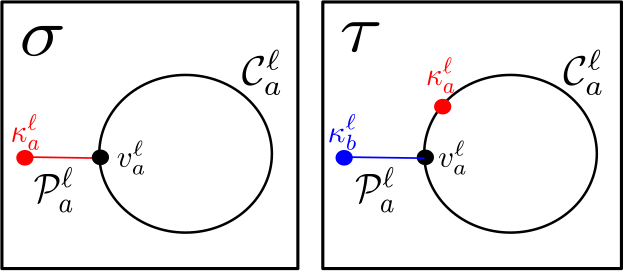
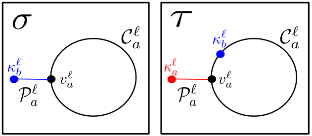
Equipped with the results of Subsection 4.2, we are now ready to establish that there are two configurations in , one of them being , with distance . The idea is to construct a series of swaps, layer-by-layer. For , each iteration on layer will require a certain number of iterations in layer . We formalize this in Definition 4.12 by a notion that we refer to as -extractions, which we illustrate in Figure 18.
Definition 4.12.
For and , we say that is an -extraction of if either:
-
(1)
and , ,
-
(2)
and , .
In other words, if is an -extraction of , one of the two partite sets of is a subset of . Then “extracts” this partite set out of and replaces it with the other partite set of , which is then a subset .
For use in the proof of Proposition 4.14, we also introduce the following definition, corresponding to knob vertices in rotating about their corresponding cycle subgraphs in . Recall from Subsection 4.1 that for all ,
Definition 4.13.
For , and a positive integer such that , a -rotation with is a swap sequence for which for all and there exists an enumeration such that for all and whenever . Similarly, for , and a positive integer such that , a -rotation with is a swap sequence for which for all and there exists an enumeration such that for all and whenever .
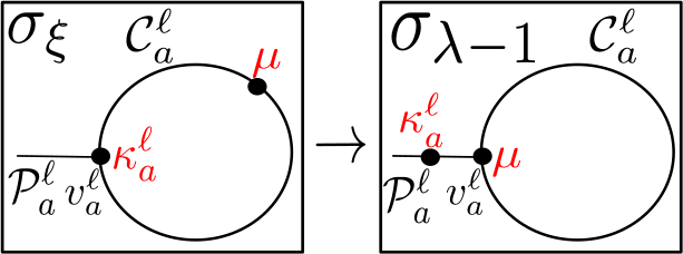
Note that Definition 4.13, which is illustrated in Figure 19, corresponds to a cyclic rotation of all elements in about the knob vertex , which is fixed in the same position since . The direction and length of this rotation depend on the enumeration of the vertices in the relevant cycle and the value , respectively.
The final configuration in for which we will argue that is going to be an -extraction of (of the kind from Definition 4.12(1)). We begin by showing that for any , -extractions of exist in . This will follow as an immediate corollary of Proposition 4.14 by taking for this value of , since is then an -extraction of .
Proposition 4.14.
For any positive integer and , there exists a swap sequence , with a subsequence , , such that
-
(1)
for every , is an -extraction of ;
-
(2)
for every and , there exists a -rotation with and -rotation with that is a contiguous subsequence of .
Proof.
We deviate from our usual practice in Subsections 4.2 and 4.3 of assuming that everything proceeds under the context of some fixed , and establish Proposition 4.14 via induction on . Specifically, we will show by induction on that for any fixed , Proposition 4.14 holds for the graphs and . During the induction step, in another deviation from our usual practice, we shall be more explicit about the pairs of graphs and the starting configurations that we reference for sake of clarity.
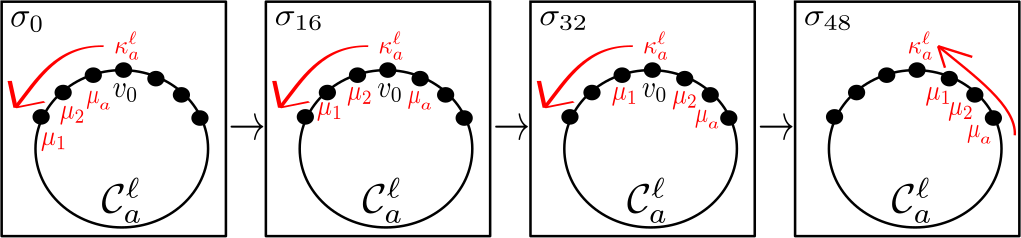
We begin with the induction basis, . Here, is the only value of for which Proposition 4.14 applies. Consider the following sequence of swaps from : Figure 20 illustrates the first three steps of this procedure.
-
(1)
Perform a -rotation with to move to .
-
(2)
Perform a -rotation with to move to .
-
(3)
Swap as far left through as possible, yielding a vertex upon .
-
(4)
Perform a -rotation with to move to .
-
(5)
Perform a -rotation with to move to .
-
(6)
Swap as far right through as possible, producing a vertex in upon .
It is straightforward to conclude that repeating this algorithm times (since ) from (adapted to the mapping upon , then the mapping upon , for subsequent iterations) yields a -extraction of , namely of the kind in Definition 4.12(1), since we have
and that for every , there exists a -rotation with and -rotation with that is a contiguous subsequence of the resulting swap sequence. It is similarly straightforward to see that we can repeat this algorithm to interchange the positions of and arbitrarily many times (i.e., for any positive integer ), with a -rotation with and -rotation with for every executed as a contiguous subsequence of every such interchange. On even iterations of this interchange, we simply switch the roles of and in the above algorithm, resulting in -extractions of the kind in Definition 4.12(2).
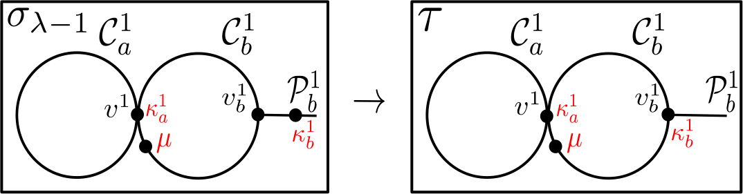
Now assume Proposition 4.14 holds for some fixed (i.e., for this fixed , Proposition 4.14 holds for the graphs and ). By the induction hypothesis applied on and , we can extract a swap sequence in with and with a subsequence satisfying Proposition 4.14. Now consider and , which has corresponding starting configuration in the connected component , which we denote and , respectively. In an abuse of notation, for the rest of the present proof we let denote the first layers of and . These subgraphs are isomorphic to the graphs and as they were originally defined during their construction in Subsection 4.1, and under these isomorphisms, restricted to can be understood to be the same as as defined in Subsection 4.1. Furthermore, the swap sequence can be understood as being in , with , if we set
As such, it follows from the induction hypothesis that Proposition 4.14 holds for if we take , and all that remains is to confirm that Proposition 4.14 holds for for . In the proceeding argument, we assume that the swap sequence we extracted above using the induction hypothesis was for . In a similar vein, given some with and from the swap sequence , define the extension of with respect to to be the configuration101010Whenever we construct such extensions in the forthcoming argument, it will be clear that they lie in . with
-
•
for all ;
-
•
for all .
We will say that we extend with respect to , and will generally apply this notion en masse to subsequences of with respect to a single configuration of .
We will now construct a swap sequence in , with , satisfying Proposition 4.14 for . This is illustrated in Figure 21. From the swap sequence , with subsequence as discussed before, consider , which, by the induction hypothesis, has a contiguous subsequence that is a -rotation with . Let be such that and : the observation that such a exists follows quickly from the restrictions of Definition 4.13. We construct a swap sequence in by merging , and , which we now define.
-
(1)
Extend with respect to , yielding .
-
(2)
Let , with , be a -rotation with , with length such that is moved to .
-
(3)
Extend with respect to , yielding .
Now take the subsequence of , which has contiguous subsequence that is a -rotation with , and such that and . Construct by merging , and , which we now define.
-
(1)
Extend with respect to , yielding .
-
(2)
Let , with , be the result of performing a -rotation with to move to , then swapping as far left as possible across , then performing a -rotation to swap the resulting vertex upon onto .
-
(3)
Extend with respect to , yielding .
It is now straightforward to see how to similarly construct the sequences , and why we took when appealing to the induction hypothesis: each sequence corresponding to a different vertex in lying on , and following , we alternate the path that we “push” this vertex through. The only modification arises when we construct : during the -rotation with within , simply include a -rotation which moves the vertex upon onto . Merging yields a sequence , such that is an -extraction of , since
It is evident by tracing the above construction that for every , there exists a -rotation with and -rotation with that is a contiguous subsequence of . Thus, the swap sequence establishes that Proposition 4.14 holds for on .
For general , we can invoke the induction hypothesis, applied to , to extract a swap sequence in with subsequence . Then we can proceed as in the case for every contiguous subsequence in , for , to construct a swap sequence which establishes Proposition 4.14 for this value of . ∎
In the proof of Proposition 4.14, during the induction basis we reached a -extraction of by performing iterations of an algorithm which executed swaps.111111Note that we inducted on in the proof of Proposition 4.14, so the sequence of swaps we found for smaller values of would be executed on subgraphs of for larger values of . However, it is easy to verify, by tracing the construction in Subsection 4.1, that the asymptotic statements here hold regardless of the fixed value of that we choose. Then in the inductive step, we reached an -extraction of by taking -extractions of and stringing them together by appending some other swap sequences. Altogether, it follows that we found a sequence of swaps to reach an -extraction of — if this were tight, taking to be as large as desired would be enough to answer Question 1.2 in the negative. Motivated by these ideas, we prove Proposition 4.15, which will lend itself to a lower bound on .
Proposition 4.15.
Fix integers and , and take such that is an -extraction of . Any swap sequence with and must have a subsequence such that, for , there exists a configuration that is an -extraction of .
Proof.
Assume is an -extraction of of the kind of Definition 4.12(1). Proposition 4.15 can be proved in the setting where is an -extraction of of the kind of Definition 4.12(2) entirely analogously, where we switch the roles of several expressions corresponding to the “left and right sides” of the subgraphs and in this case.
We will say that is the initial subgraph of any vertex ( if ) with . By Proposition 4.6(3), leaving the initial subgraph corresponds to an -friendly swap where is upon and swaps onto some vertex in . Similarly, is the initial subgraph for ( if ) with . By Proposition 4.6(3), leaving the initial subgraph corresponds to an -friendly swap where is upon and swaps onto some vertex in .
Let be a swap sequence with and . It is straightforward to show from Proposition 4.6(4) and Definition 4.12(1) that at least vertices in ( for ) switch to the “opposite” layer subgraph in over the course of . Take any such vertices , indexed in the order that they first leave their initial subgraph during (it is clear that at most one such vertex can leave their initial subgraph over a given swap). Construct a subsequence of such that, for every , is the smallest index for which
-
•
;
-
•
is not a vertex in the initial subgraph of .
Consider any for which . The neighborhood of is
The vertex that swaps with to reach from satisfies
since would violate Proposition 4.6(4) (on layer ) if we had that . Assume (towards a contradiction) that , and let (the lower bound is since ) be the smallest such index satisfying
| (4.27) |
Exactly one of the two statements
-
•
;
-
•
is true; both being false would contradict being the smallest possible, while both being true would contradict being the smallest possible. But would imply that violates Proposition 4.4 (on ), and would imply that violates Proposition 4.6(4) (on layer if it swaps with , and on layer if it swaps with a vertex in ). So for all ,
| (4.28) |
where the latter claim can be deduced from an entirely analogous argument. See Figure 22 for an illustration.
Now consider for which . For such values of which have that , establishing the existence of a configuration that is an -extraction of can be done entirely analogously. By (4.28), , so certainly
and since ,
By Proposition 4.11(2),
| (4.29) |
If it were true that , there would exist satisfying . Combined with (4.29), we would have
| (4.30) |
since the LHS is a subset of the RHS and their cardinalities are equal. In particular, it must be that , so Proposition 4.8(2) would imply that
so there exists that is in , contradicting (4.30). So it must be that , i.e., that
| (4.31) |
If , then (4.28) implies , and so
Proposition 4.11(1) thus implies
This statement, with (4.29) and (4.31), implies that is an -extraction of , namely of the Definition 4.12(2) kind. If , then (4.28) implies , so
Proposition 4.11(2) now implies that
Since is the smallest possible, , and it follows that , as would otherwise violate Proposition 4.6(4) on layer (due to and ). It is straightforward to confirm, appealing to Proposition 4.4 on , that moves to during , and swaps with upon at some point in this swap sequence.121212This can be proved using ideas and arguments which are essentially identical to those that were carried out in Subcase 1.2 of the proof of Proposition 4.6. Thus, there exists a configuration for which
from which it immediately follows that
and Proposition 4.11(1) implies
This, with (4.29) and (4.31), implies that is an -extraction of , namely of the Definition 4.12(2) kind.
Therefore, taking yields the desired subsequence of . ∎
4.4. Proof of Theorem 1.3
We finally derive the desired lower bound on the diameter of .
See 1.3
Proof.
For , take , on vertices (see Subsection 4.1). For , define
| (4.32) |
It follows from Proposition 4.15 that for all ,
| (4.33) |
Let be such that is an -extraction of , which exists by Proposition 4.14. By (4.32) and (4.33),
Now, for , fix (here, ), and construct -vertex graphs , by adding isolated vertices to and , respectively. Let , denote the connected component of , containing the configuration resulting from placing upon as usual (i.e., under the starting configuration as defined in Subsection 4.1), and then placing the isolated vertices in upon the isolated vertices of in some way. It easily follows from our construction that , so
By accounting for the values , which may weaken the constant implicit in the term, the desired result now follows immediately. ∎
To conclude Section 4, we mention an especially notable implication of Theorem 1.3 in the study of random walks on friends-and-strangers graphs. In the proceeding discussion, to avoid distracting from the nature of this article, we elect to be terse and do not define many of the objects we consider; we refer the reader to [Lov93] for a thorough treatment of random walks on graphs. We begin by providing the following Definition 4.16. The fact that there is a natural discrete-time Markov chain associated to a friends-and-strangers graph was observed in passing in [ADK23, Section 7], and an investigation of its mixing properties was separately proposed in [Alo21].
Definition 4.16.
Let and be -vertex graphs. The friends-and-strangers Markov chain of and is the discrete-time Markov chain whose state space is and such that at each time step, a pair of friends standing upon adjacent vertices is chosen uniformly at random amongst all such pairs and swap places with probability .
The friends-and-strangers Markov chain of and , which models a lazy random walk on a connected component of , is aperiodic by construction (recall from Proposition 2.3(2) that friends-and-strangers graphs are bipartite, which warrants the laziness condition in Definition 4.16 if we would like to discuss mixing to stationarity) and irreducible when restricted to a connected component of . From a different perspective, Definition 4.16 may be interpreted as the generalization of a natural discrete variant of the interchange process131313The interchange process is usually posed as a continuous-time stochastic process by assigning, to the edges of , independent point processes on the positive half-line, and transposing the particles upon the vertices incident to a given edge at the points of its corresponding process. One can certainly adapt Definition 4.16 to accommodate for such differences in the presentation of the model. (sometimes called the random stirring process) where we include the condition that arbitrary pairs of particles may be forbidden from swapping positions. The friends-and-strangers Markov chain has received substantial attention under certain restricted settings (chiefly that in which ), and classical polynomial upper bounds on the mixing time (in total variation distance) of the underlying Markov chain are known; see [Ald83, AD86, DS81, DS93, Jon12, Mat88, Wil04]. An immediate corollary of Theorem 1.3, which might be thought of as its natural stochastic analogue (especially in light of the polynomial upper bounds that we derived in Section 3), is the following.
Corollary 4.17.
For all , there exist -vertex graphs and for which there exists a connected component of such that the friends-and-strangers Markov chain of and , when restricted to this component, has mixing time (in total variation distance) which is .
In other words, for this variant of the interchange process in which we may further forbid certain pairs of particles from swapping places with each other, it is possible to fix restrictions between particles in such a way that the mixing time of the underlying Markov chain is exponential in the size of the graph on which the process occurs. This is in stark contrast to the aforementioned polynomial upper bounds regarding rapidly mixing Markov chains.
5. Open Questions and Future Directions
Theorem 1.3 of this paper proves that diameters of connected components of friends-and-strangers graphs may grow exponentially in the size of their input graphs. There are many other interesting questions concerning distance and diameter that remain unresolved by this article.
5.1. Other Choices of Fixed Graphs
In Section 3, we fixed to be from a particular class of graphs, and derived bounds on the maximal diameter of a connected component . Of course, we could pursue similar inquiries for other choices of . One natural choice would be to take . It is known (see [Bin+23]) that the diameter of any component of is at most , but to our knowledge, there are no known bounds on the maximum diameter for general . We also remark that it may be possible to extract a bound on the maximum diameter of a component of for biconnected graphs by tracing the arguments in [Wil74].
5.2. Improvements
For much of our discussion in Subsection 3.3, we were primarily interested in showing that the maximum diameter of a connected component of was polynomially bounded (in the sense of Question 1.2), rather than achieving tight asymptotic statements. It would be desirable to improve these results, toward which we pose the following conjectures. We mention that generalizing the lattice-theoretic methods of [Pro21], which are of a very different flavor than the arguments presented here, might lead to the resolution of Conjecture 5.2. We also note that if Conjecture 5.1 were settled, then tracing the proof of Corollary 3.10 would immediately lead to an bound on the number of double-flips needed to go between double-flip equivalent acyclic orientations and on an -vertex graph, sharpening Corollary 3.10.
Conjecture 5.1.
The maximum diameter of a connected component of is .
Conjecture 5.2.
For an -vertex graph and two acyclic orientations that are double-flip equivalent, it is possible to go from to in double-flips.
In another direction, Theorem 1.3 states that for all , there exist -vertex and such that the maximum diameter of a connected component of is . It is unclear how close this is to the truth. As a first step, we pose the following problem.
Question 5.3.
For -vertex graphs and , does there exist a nontrivial upper bound (in terms of ) on the maximum diameter of a component of ?
We briefly clarify what we mean by a nontrivial upper bound in Question 5.3. Let denote the maximum possible diameter of a connected component of when and are -vertex graphs. By Theorem 1.3 for the lower bound and Stirling’s approximation applied to for the upper bound, we observe that
Thus, our understanding of is tight up to a logarithmic factor in the exponent. Any improvement over this naive upper bound, or confirmation that this upper bound is essentially the truth, would be highly desirable. In particular, we ask the following more precise question. Indeed, given the preceding discussion, Question 5.4 is the natural next target.
Question 5.4.
Is it true that ?
We propose one final problem in this subsection which we would especially like to see resolved.
Problem 5.5.
Find a shorter (perhaps via non-constructive141414Certainly, a proof of Theorem 1.3 using non-constructive techniques would be a novel contribution. In another direction, recall that the central idea behind Section 4 was to construct an exponentially increasing recursive sequence of swaps in such a way that executing this sequence of swaps is necessary in order to reach one configuration from another. A constructive proof which either proceeds via a similar paradigm with a construction that is more amenable to analysis or leverages different ideas altogether would also be of interest. means) proof of Theorem 1.3.
5.3. Connected Friends-and-Strangers Graphs
The proof of Theorem 1.3 relied heavily on characterizing all vertices of in the same connected component of . It is thus natural to ask Question 1.2 in the setting where is assumed to be connected, which was separately raised by Defant and Kravitz.
Question 5.6 ([DK21, Subsection 7.3]).
Does there exist an absolute constant such that for all -vertex graphs and with connected, it holds that is ?
If Question 5.6 holds in the negative, then settling it will likely require very different techniques and paradigms than those which were developed in this article. Indeed, the proof of the negative result for Question 1.2 relies heavily on “rigging” the configurations that lie in a particular connected component of , which allows us to argue that two particular configurations (namely, and ) are necessarily very far apart. Such a strategy is not applicable if we require to be connected. Additionally, by Proposition 2.3(3), we can assume (without loss of generality) that is biconnected under this setting, and that either or has no cut vertices. Theorem 3.7 already gives a positive result for , the “simplest” biconnected graph (e.g., the -vertex cycle has the smallest Betti number amongst all -vertex biconnected graphs: see [Whi31, Theorem 19], which might lend itself to an inductive argument) and for , the most “complicated” ( has the largest Betti number amongst all -vertex biconnected graphs). Furthermore, the constructions and contain cut vertices which hold central roles in the proofs of the intermediate propositions (namely, vertices on the paths for , and the knob vertices in ).
In another direction, a negative answer to Question 5.6 implies the existence of long paths in the connected graph . The following result shows that the extreme end of this is not possible.
Proposition 5.7.
For , is not isomorphic to a tree on vertices (e.g., ) or a tree on vertices with one edge appended (e.g., ).
Proof.
The number of edges of is , while this is and for a tree on vertices and a tree with one edge appended on vertices, respectively. Notice that is divisible by while is not, so cannot be isomorphic to a tree on vertices. Assume is isomorphic to a tree with an edge appended to it, so , or . Then and must both be connected, so that (without loss of generality) and , so is a tree. Due to Proposition 2.3(3), is biconnected, so necessarily . But , contradicting Theorem 2.6, which gives . ∎
5.4. Probabilistic Problems
In a different direction, we may study notions of distance in friends-and-strangers graphs when we take and to be random graphs. We propose the following problem; we leave the meaning of “small diameter” up to interpretation.
Problem 5.8.
Let and be independently-chosen random graphs from . Find conditions on (in terms of ) which guarantee that every connected component of has small diameter with high probability.
We also restate a problem of this kind proposed by [ADK23].
Problem 5.9 ([ADK23, Problem 7.9]).
Obtain estimates (in terms of and ) for the expectation of the maximum diameter of a connected component in when and are independently-chosen random graphs from .
In a manner analogous to how we fixed one of the two graphs and in Section 3 and studied the resulting variant of Question 1.2 before addressing the more global question, it may be insightful to first fix (without loss of generality) to be a particular kind of graph and study the variants of Problems 5.8 and 5.9 which only take to be drawn from . The graphs we studied in Section 3 (complete graphs, paths, and cycles) may also serve as natural starting points here.
5.5. Complexity
As the literature on the token swapping problem suggests, computing exact distances between two configurations in and the maximum diameter of a component of , under mild assumptions on and , seems to be intractable. We might thus study distances and diameters in friends-and-strangers graphs from the perspective of complexity theory. We discuss one possible direction of study along these lines here. We start by introducing a decision problem which encapsulates finding the shortest swap sequence between two configurations.
Definition 5.10.
In an instance of the distance problem, we are given graphs and on vertices, configurations , and a positive integer , and want to know if .
This problem has been studied in many restricted contexts. If we proceed under the assumption that , the distance problem is known to be PSPACE-complete [Jer85], APX-hard [Mil+16], and -hard when parametrized by the shortest number of swaps [BMR18]. Furthermore, it is NP-hard when we impose certain additional restrictions, such as when we take to be a tree and [Aic+22]. It might be fruitful to study the complexity of this problem at the level of generality proposed by Definition 5.10.
A natural follow-up to Definition 5.10 is to ask for worst-case distances between two configurations, which corresponds to the maximum diameter of a component of .
Definition 5.11.
In an instance of the diameter problem, we are given graphs and on vertices and a positive integer , and want to know if the maximum diameter of a component of is at most .
The literature suggests that the diameter problem has not been studied as thoroughly as the distance problem, even when assuming that one of the two graphs is complete. Towards bridging this gap, we pose the following primitive question and problem.
Question 5.12.
Is the diameter problem in EXPSPACE? If so, is it EXPSPACE-complete? What changes if we fix ?
Problem 5.13.
Find assumptions on , , and which guarantee that the diameter problem (under these assumptions) is in PSPACE.
Notably, even simpler decision problems than those proposed in Definitions 5.10 and 5.11 seem to be poorly understood. For instance, we may consider the following decision problems.
Definition 5.14.
In an instance of the component problem, we are given -vertex graphs and and configurations , and want to know if and lie in the same connected component of .
Definition 5.15.
In an instance of the connectivity problem, we are given -vertex graphs and , and want to know if is connected.
We may think of the component problem and the connectivity problem as, respectively, the simplest instances of the distance problem (asking whether is finite) and of the diameter problem (asking whether the diameter of , when we do not restrict to connected components, is finite). To our knowledge, an understanding of the complexity of the component problem and the connectivity problem remains open, though the results in [Ala+23] address these problems when studying friends-and-strangers graphs with multiplicities, as elaborated in [Mil23].
In a different direction, [AK89, VP95, Yam+15] independently found -approximation algorithms for determining the distance between two configurations in when is a tree. Recall from the proof of Proposition 3.2 that for any in the same connected component, , and an algorithm which exactly computes the distance between any two configurations in is one which, starting from , reverses a -inversion at every step. These two observations naturally suggest the following problem, which one can also pursue by replacing with a different fixed graph.
Problem 5.16.
Find, under the most general assumptions on possible, an -approximation algorithm for computing the distance between two configurations in .
Acknowledgments
This research was initiated at the University of Minnesota Duluth REU and was supported, in part, by NSF-DMS grant 1949884 and NSA Grant H98230-20-1-0009. I would like to thank Professor Joseph Gallian for organizing the Duluth REU and for giving me a chance to participate in his 2021 program, and I am deeply grateful to Colin Defant and Noah Kravitz for suggesting these problems to me and for many helpful conversations over the course of that summer. In particular, I thank Colin Defant for carefully reading through a draft of this article, providing many productive comments on the manuscript. I also thank Yelena Mandelshtam for reviewing a draft of this work and providing constructive feedback. Finally, I would like to sincerely thank the two anonymous referees for thoroughly reviewing an earlier draft of this work, catching many typos and grammatical mistakes, and providing many detailed comments and suggestions which have vastly improved this article’s clarity. Notably, I am immensely grateful to the anonymous referee who proposed a simple way to sharpen the main result of this paper.
References
References
- [AD86] David Aldous and Persi Diaconis “Shuffling cards and stopping times” In The American Mathematical Monthly 93.5 Taylor & Francis, 1986, pp. 333–348
- [ADK23] Noga Alon, Colin Defant and Noah Kravitz “Typical and extremal aspects of friends-and-strangers graphs” In Journal of Combinatorial Theory, Series B 158.1 Elsevier, 2023, pp. 3–42
- [AF02] David Aldous and Jim Fill “Reversible Markov chains and random walks on graphs” Berkeley, 2002 URL: https://www.stat.berkeley.edu/~aldous/RWG/book.html
- [Aic+22] Oswin Aichholzer, Erik D Demaine, Matias Korman, Jayson Lynch, Anna Lubiw, Zuzana Masárová, Mikhail Rudoy, Virginia Vassilevska Williams and Nicole Wein “Hardness of token swapping on trees” In 30th Annual European Symposium on Algorithms, 2022, pp. 33:1–33:15
- [AK13] Gil Alon and Gady Kozma “The probability of long cycles in interchange processes” In Duke Mathematical Journal 162.9 Duke University Press, 2013, pp. 1567–1585
- [AK89] Sheldon B. Akers and Balakrishnan Krishnamurthy “A group-theoretic model for symmetric interconnection networks” In IEEE Transactions on Computers 38.4 IEEE, 1989, pp. 555–566
- [Ala+23] Robert M. Alaniz, Josh Brunner, Michael Coulombe, Erik D. Demaine, Jenny Diomidova, Ryan Knobel, Timothy Gomez, Elise Grizzell, Jayson Lynch, Andrew Rodriguez, Robert Schweller and Tim Wylie “Complexity of Reconfiguration in Surface Chemical Reaction Networks”, 2023 arXiv:2303.15556 [cs.CC]
- [Ald83] David Aldous “Random walks on finite groups and rapidly mixing Markov chains” In Séminaire de Probabilités XVII 1981/82: Proceedings, 1983, pp. 243–297 Springer
- [Alo21] Noga Alon “Random friends walking on random graphs”, 2021 Talk given at the Oxford Discrete MathsProbability Seminar URL: https://www.youtube.com/watch?v=uheP2ctJx10
- [Ang03] Omer Angel “Random infinite permutations and the cyclic time random walk” In Discrete Mathematics & Theoretical Computer Science Episciences. org, 2003
- [Ban22] Kiril Bangachev “On the asymmetric generalizations of two extremal questions on friends-and-strangers graphs” In European Journal of Combinatorics 104 Elsevier, 2022, pp. 103529
- [BD06] Nathanaël Berestycki and Rick Durrett “A phase transition in the random transposition random walk” In Probability theory and related fields 136 Springer, 2006, pp. 203–233
- [BE78] Béla Bollobás and Stephen E Eldridge “Packings of graphs and applications to computational complexity” In Journal of Combinatorial Theory, Series B 25.2 Elsevier, 1978, pp. 105–124
- [Bin+23] Ahmad Biniaz, Kshitij Jain, Anna Lubiw, Zuzana Masárová, Tillmann Miltzow, Debajyoti Mondal, Anurag Murty Naredla, Josef Tkadlec and Alexi Turcotte “Token Swapping on Trees” In Discrete Mathematics & Theoretical Computer Science 24.2 Episciences.org, 2023
- [BK23] Florestan Brunck and Matthew Kwan “Books, Hallways and Social Butterflies: A Note on Sliding Block Puzzles”, 2023 arXiv:2303.09459 [math.CO]
- [BMR18] Édouard Bonnet, Tillmann Miltzow and Paweł Rzkażewski “Complexity of token swapping and its variants” In Algorithmica 80 Springer, 2018, pp. 2656–2682
- [BR99] Christopher L Barrett and Christian M Reidys “Elements of a theory of computer simulation I: sequential CA over random graphs” In Applied Mathematics and Computation 98.2-3 Elsevier, 1999, pp. 241–259
- [Bra+19] Tatiana Brailovskaya, Gokul Gowri, Sean Yu and Erik Winfree “Reversible computation using swap reactions on a surface” In DNA Computing and Molecular Programming: 25th International Conference, DNA 25, Seattle, WA, USA, August 5–9, 2019, Proceedings 25, 2019, pp. 174–196 Springer
- [Cay49] Arthur Cayley “LXXVII. Note on the theory of permutations” In The London, Edinburgh, and Dublin Philosophical Magazine and Journal of Science 34.232 Taylor & Francis, 1849, pp. 527–529
- [Che10] Beifang Chen “Orientations, lattice polytopes, and group arrangements I: Chromatic and tension polynomials of graphs” In Annals of Combinatorics 13 Springer, 2010, pp. 425–452
- [CLR10] Pietro Caputo, Thomas Liggett and Thomas Richthammer “Proof of Aldous’ spectral gap conjecture” In Journal of the American Mathematical Society 23.3, 2010, pp. 831–851
- [Def+22] Colin Defant, David Dong, Alan Lee and Michelle Wei “Connectedness and Cycle Spaces of Friends-and-Strangers Graphs”, 2022 arXiv:2209.01704 [math.CO]
- [DK21] Colin Defant and Noah Kravitz “Friends and strangers walking on graphs” In Combinatorial Theory, 1 (0), 2021
- [DMR16] Mike Develin, Matthew Macauley and Victor Reiner “Toric partial orders” In Transactions of the American Mathematical Society 368.4, 2016, pp. 2263–2287
- [DR18] Erik D Demaine and Mikhail Rudoy “A simple proof that the -puzzle is hard” In Theoretical Computer Science 732 Elsevier, 2018, pp. 80–84
- [DS81] Persi Diaconis and Mehrdad Shahshahani “Generating a random permutation with random transpositions” In Zeitschrift für Wahrscheinlichkeitstheorie und verwandte Gebiete 57.2 Springer, 1981, pp. 159–179
- [DS93] Persi Diaconis and Laurent Saloff-Coste “Comparison techniques for random walk on finite groups” In The Annals of Probability JSTOR, 1993, pp. 2131–2156
- [ES23] Dor Elboim and Allan Sly “Infinite cycles in the interchange process in five dimensions”, 2023 arXiv:2211.17023 [math.PR]
- [Ham15] Alan Hammond “Sharp phase transition in the random stirring model on trees” In Probability Theory and Related Fields 161 Springer, 2015, pp. 429–448
- [HS21] Jonathan Hermon and Justin Salez “The interchange process on high-dimensional products” In Annals of Applied Probability 31.1, 2021
- [Jeo22] Ryan Jeong “On Structural Aspects of Friends-And-Strangers Graphs” To appear in the Annals of Combinatorics, 2022 arXiv:2203.10337 [math.CO]
- [Jeo23] Ryan Jeong “Bipartite Friends and Strangers Walking on Bipartite Graphs”, 2023 arXiv:2309.03848 [math.CO]
- [Jer85] Mark R Jerrum “The complexity of finding minimum-length generator sequences” In Theoretical Computer Science 36 Elsevier, 1985, pp. 265–289
- [Jon12] Johan Jonasson “Mixing times for the interchange process” In ALEA 9.2, 2012, pp. 667–683
- [Kim16] Dohan Kim “Sorting on graphs by adjacent swaps using permutation groups” In Computer Science Review 22 Elsevier, 2016, pp. 89–105
- [KMS84] D. Kornhauser, G. Miller and P. Spirakis “Coordinating Pebble Motion On Graphs, The Diameter Of Permutation Groups, And Applications” In 25th Annual Symposium on Foundations of Computer Science, 1984., 1984, pp. 241–250
- [KO09] Daniela Kühn and Deryk Osthus “The minimum degree threshold for perfect graph packings” In Combinatorica 29.1 Springer, 2009, pp. 65–107
- [KSY19] Jun Kawahara, Toshiki Saitoh and Ryo Yoshinaka “The time complexity of permutation routing via matching, token swapping and a variant” In Journal of Graph Algorithms and Applications 23.1, 2019, pp. 29–70
- [Lee22] Alan Lee “Connectedness in Friends-and-Strangers Graphs of Spiders and Complements”, 2022 arXiv:2210.04768 [math.CO]
- [Lov93] L Lovász “Random walks on graphs: a survey” In J. Bolyai Math. Soc. 2, 1993, pp. 1–46
- [Mat88] Peter Matthews “A strong uniform time for random transpositions” In Journal of Theoretical Probability 1 Springer, 1988, pp. 411–423
- [Mil+16] Tillmann Miltzow, Lothar Narins, Yoshio Okamoto, Günter Rote, Antonis Thomas and Takeaki Uno “Approximation and Hardness of Token Swapping” In 24th Annual European Symposium on Algorithms 57, 2016, pp. 66:1–66:15
- [Mil23] Aleksa Milojevic “Connectivity of Old and New Models of Friends-and-Strangers Graphs”, 2023 arXiv:2210.03864 [math.CO]
- [MM11] Matthew Macauley and Henning S Mortveit “Posets from Admissible Coxeter Sequences” In The Electronic Journal of Combinatorics 18.1, 2011, pp. P197
- [Naa00] Michael Naatz “The graph of linear extensions revisited” In SIAM Journal on Discrete Mathematics 13.3 SIAM, 2000, pp. 354–369
- [Par15] Ian Parberry “Solving the -Puzzle with Expected Moves” In Algorithms 8.3 MDPI, 2015, pp. 459–465
- [Pre86] Oliver Pretzel “On reorienting graphs by pushing down maximal vertices” In Order 3.2 Springer, 1986, pp. 135–153
- [Pro21] James Propp “Lattice structure for orientations of graphs”, 2021 arXiv:math/0209005 [math.CO]
- [PV90] Frederick J Portier and Theresa P Vaughan “Whitney numbers of the second kind for the star poset” In European Journal of Combinatorics 11.3 Elsevier, 1990, pp. 277–288
- [Rei98] CM Reidys “Acyclic orientations of random graphs” In Advances in Applied Mathematics 21.2 Elsevier, 1998, pp. 181–192
- [Sch05] Oded Schramm “Compositions of random transpositions” In Israel Journal of Mathematics 147 Springer, 2005, pp. 221–243
- [Spe09] David Speyer “Powers of Coxeter elements in infinite groups are reduced” In Proceedings of the American Mathematical Society 137.4, 2009, pp. 1295–1302
- [SS78] Norbert Sauer and Joel Spencer “Edge disjoint placement of graphs” In Journal of Combinatorial Theory, Series B 25.3 Academic Press, 1978, pp. 295–302
- [Sta08] Richard P Stanley “An equivalence relation on the symmetric group and multiplicity-free flag h-vectors” In Journal of Combinatorics 0.0, 2008
- [van+16] Anke van Zuylen, James Bieron, Frans Schalekamp and Gexin Yu “A tight upper bound on the number of cyclically adjacent transpositions to sort a permutation” In Information Processing Letters 116.11, 2016, pp. 718–722
- [VP95] Theresa P Vaughan and Frederick J Portier “An algorithm for the factorization of permutations on a tree” In Journal of Combinatorial Mathematics and Combinatorial Computing 18, 1995, pp. 11–31
- [WC23] Lanchao Wang and Yaojun Chen “Connectivity of friends-and-strangers graphs on random pairs” In Discrete Mathematics 346.3 Elsevier, 2023, pp. 113266
- [Whi31] Hassler Whitney “Non-separable and planar graphs” In Proceedings of the National Academy of Sciences 17.2 National Acad Sciences, 1931, pp. 125–127
- [Wil04] David Bruce Wilson “Mixing times of lozenge tiling and card shuffling Markov chains” In The Annals of Applied Probability 14.1 Institute of Mathematical Statistics, 2004, pp. 274–325
- [Wil74] Richard M Wilson “Graph puzzles, homotopy, and the alternating group” In Journal of Combinatorial Theory, Series B 16.1 Elsevier, 1974, pp. 86–96
- [WLC23] Lanchao Wang, Junying Lu and Yaojun Chen “Connectedness of friends-and-strangers graphs of complete bipartite graphs and others” In Discrete Mathematics 346.8, 2023, pp. 113499
- [Yam+15] Katsuhisa Yamanaka, Erik D Demaine, Takehiro Ito, Jun Kawahara, Masashi Kiyomi, Yoshio Okamoto, Toshiki Saitoh, Akira Suzuki, Kei Uchizawa and Takeaki Uno “Swapping labeled tokens on graphs” In Theoretical Computer Science 586 Elsevier, 2015, pp. 81–94
- [Yan11] Chao Yang “Sliding puzzles and rotating puzzles on graphs” In Discrete Mathematics 311.14 Elsevier, 2011, pp. 1290–1294
- [Yap88] HP Yap “Packing of graphs-a survey” In Annals of Discrete Mathematics 38 Elsevier, 1988, pp. 395–404
- [Yus07] Raphael Yuster “Combinatorial and computational aspects of graph packing and graph decomposition” In Computer Science Review 1.1 Elsevier, 2007, pp. 12–26
- [Zhu23] Honglin Zhu “Evacuating ”O”- and ”Y”-shaped houses on fire: the connectivity of friends-and-strangers graphs on complete multipartite graphs”, 2023 arXiv:2307.08121 [math.CO]