On the dynamical kernels of fermionic equations of motion in strongly-correlated media
Abstract
Two-point fermionic propagators in strongly correlated media are considered with an emphasis on the dynamical interaction kernels of their equations of motion (EOM). With the many-body Hamiltonian confined by a two-body interaction, the EOMs for the two-point fermionic propagators acquire the Dyson form and, before taking any approximation, the interaction kernels decompose into the static and dynamical (time-dependent) contributions. The latter translate to the energy-dependent and the former map to the energy-independent terms in the energy domain. We dwell particularly on the energy-dependent terms, which generate long-range correlations while making feedback on their short-range static counterparts. The origin, forms, and various approximations for the dynamical kernels of one-fermion and two-fermion propagators, most relevant in the intermediate-coupling regime, are discussed. Applications to the electromagnetic dipole response of 68,70Ni and low-energy quadrupole response of 114,116,124Sn are presented.
I Introduction
Finding accurate quantitative solutions to the nuclear many-body problem has remained an active field of research for decades. Challenged by the requirements of various applications in nuclear science and technology and driven by the newly emerging computational capabilities, it shows substantial progress over the years, however, predictive computation of atomic nuclei calls for further developments on the theoretical side.
One of the most powerful tools to study atomic nuclei and, more generally, strongly correlated fermionic many-body systems is the Green function method. Various Green functions, or propagators, belonging to a larger class of correlation functions (CFs), form a common theoretical background across the energy scales. The Green functions are directly related to well-defined observables Matsubara (1955); Watson (1956); Brueckner and Levinson (1955); Brueckner (1955); Martin and Schwinger (1959); Ethofer (1969); Schuck and Ethofer (1973). In particular, the single-nucleon propagators are linked to the energies of odd-particle systems and spectroscopic factors which, in the case of atomic nuclei, can be extracted from, e.g., transfer or knock-out reactions. The two-nucleon particle-hole propagators are associated with the response to external probes of electromagnetic, strong, or weak character. Superfluidity can be efficiently described by two-particle in-medium pair propagators associated with pair transfer, while the residues of those propagators can be related to the pairing gaps Gorkov (1958); Kadanoff and Martin (1961).
While these propagators are mostly relevant to the observed phenomena, higher-rank CFs appear as part of the general theory in the dynamical kernels of the equations of motion (EOMs) describing the lower-rank ones Martin and Schwinger (1959); Ethofer (1969); Ethofer and Schuck (1969); Schuck and Ethofer (1973). The higher-rank propagators quantify the dynamical in-medium effects of long-range correlations thus promoting the connections between the degrees of freedom across the energy scales. They are the source of coupling between EOMs for propagators of all ranks allowable in the given system into a hierarchy, which can be decoupled by making certain approximations. Note here that the famous EOM method of Rowe Rowe (1968) operating directly bosonic excitation operators shows similar features and can be viewed as a counterpart to the Green function method. Besides the perturbative treatment, useful mostly in weak-coupling limit, the EOMs can be decoupled by cluster decompositions of their dynamical kernels in either non-symmetric Gorkov (1958); Martin and Schwinger (1959) or symmetric Schuck (1976); Adachi and Schuck (1989); Danielewicz and Schuck (1994); Dukelsky et al. (1998) forms, with varied correlation content.
Certain advantages of the symmetric forms of the dynamical kernels in the context of their cluster decompositions were particularly pointed out and elaborated by Peter Schuck and coauthors Adachi and Schuck (1989); Danielewicz and Schuck (1994); Dukelsky et al. (1998). Considering symmetric kernels was especially insightful for finding advanced solutions to the quantum many-body problem, with applications ranging from nuclear structure Litvinova and Schuck (2019) to quantum chemistry and condensed matter physics Tiago et al. (2008); Martinez et al. (2010); Sangalli et al. (2011); Schuck and Tohyama (2016a); Olevano et al. (2018), see the recent review Schuck et al. (2021) devoted to a systematic assessment of the EOM method.
Based on the progress of the nuclear many-body theory throughout the decades, recently it was demonstrated that beyond-mean-field (BMF) approaches actively employed in nuclear structure physics can be consistently linked to the Hamiltonians operating bare fermionic interactions Litvinova and Schuck (2019); Schuck (2019); Schuck et al. (2021); Litvinova and Schuck (2020, 2021). Of particular interest are the BMF approaches which account for emergent collective effects of the nuclear medium, first of all, the correlated pairs of quasiparticles known as phonons (vibrations). The phonons are shown to be derived ab-initio, and the phenomenological BMF approaches introducing phonons as part of their input, such as the nuclear field theory (NFT) Bohr and Mottelson (1969, 1975); Broglia and Bortignon (1976); Bortignon et al. (1977); Bertsch et al. (1983), its variants Tselyaev (1989); Litvinova and Tselyaev (2007) and the quasiparticle-phonon models (QPM) Soloviev (1992); Malov and Soloviev (1976), follow with the replacement of the bare fermionic interactions by effective interactions derived, e.g., from the density functional theories (DFTs). The procedure to correct the interaction kernel by subtraction of the Pauli-Villars type Tselyaev (2013) recovering the static limit of the kernel allows one to avoid inconsistencies associated with this replacement in the self-consistent implementations of the response theory Litvinova et al. (2007a, 2008, 2010, 2013); Tselyaev et al. (2018); Litvinova and Schuck (2019); Litvinova (2023).
Furthermore, the single-fermion ab-initio EOM method has been formulated for the superfluid case Litvinova and Zhang (2021). Although some versions of such an extension were available in the literature, they were either based on the phenomenological assumptions about the dynamical kernel Van der Sluys et al. (1993); Avdeenkov and Kamerdzhiev (1999); Avdeenkov and Kamerdzhev (1999); Barranco et al. (1999, 2005); Tselyaev (2007); Litvinova and Afanasjev (2011); Litvinova (2012); Afanasjev and Litvinova (2015); Idini et al. (2015) or used truncation on the one-body level to approximate it Soma et al. (2011, 2013, 2014); Somà et al. (2021). It was demonstrated in Ref. Litvinova and Zhang (2021), in particular, how pairing correlations beyond the Hartree-Fock-Bogoliubov approximation are integrated into ab-initio theory with the dynamical kernel keeping the two-fermion CFs responsible for the leading effects of emergent collectivity. In contrast to the approaches employing the Bardeen-Cooper-Schrieffer (BCS) or canonical basis, the exact single-fermion EOM was transformed to the basis of the Bogoliubov quasiparticles. This transformation has allowed for consistent unification of the normal and pairing phonon modes and considerable compactification of the superfluid Dyson equation in a more general framework. Remarkably, this enables more efficient handling of the dynamical kernels extending beyond HFB than those of the Gor’kov Green functions and a clear link of the quasiparticle-vibration coupling (qPVC) vertices to the variations of the Bogoliubov quasiparticle Hamiltonian. In Ref. Litvinova and Zhang (2022) this formulation was employed for the EOM of the response function, which has been worked out in the basis of Bogoliubov quasiparticles from the beginning, leading to a comprehensive ab-initio response theory for superfluid fermionic systems. The qPVC approaches which varying correlation content were derived and shown to generate the known phenomenological approaches, such as the second RPA, NFT, and its extensions, in certain limits. Thus, Ref. Litvinova and Zhang (2022) has paved the way toward a response theory of spectroscopic accuracy.
In this article, we discuss these recent developments and their implementations for nuclear structure calculations, where the dynamical kernels accounting for emergent collectivity play an important role. In the existing implementations of the nuclear response theory for medium-heavy nuclei, such kernels introduce correlations beyond the simplistic random phase approximation (RPA) and include up to (correlated) two-particle-two-hole () Litvinova et al. (2008, 2010); Gambacurta et al. (2011, 2015); Niu et al. (2014, 2015); Robin and Litvinova (2016); Tselyaev et al. (2018); Robin and Litvinova (2019) configuration complexity, in rare cases the one up to high energy Litvinova and Schuck (2019) or in low-energy limited Ponomarev (1999); Lo Iudice et al. (2012); Savran et al. (2011); Tsoneva et al. (2019); Lenske and Tsoneva (2019) model spaces with the current computational capabilities. These are the approaches mostly based on effective NN-interactions, either schematic or derived from the DFTs, although beyond-RPA approaches employing bare interactions also become available for light and increasingly heavier nuclei Papakonstantinou and Roth (2009); Bianco et al. (2012); Bacca et al. (2013); Knapp et al. (2014); Bacca (2014); Knapp et al. (2015); De Gregorio et al. (2016a, b); Raimondi and Barbieri (2019). An overarching goal is to develop a universal approach demonstrating consistent performance of spectroscopic accuracy across the nuclear chart, and the effort toward it includes advancements in its two major building blocks: (i) the nucleon-nucleon (NN) interactions and (ii) the quantum many-body techniques. In this work, we focus on the latter aspect for accurate modeling of the in-medium dynamics of nucleons using NN interactions as an input to the theory.
Special emphasis is put on the recent developments of the nuclear many-body problem elaborated and inspired by the scientific work of Peter Schuck. We derive the exact forms of both the static and dynamical kernels of the one-fermion and two-fermion propagators, from which all the models follow. The major focus is then placed on the approximations to the dynamical kernels, where the many-body problem is truncated on the two-body level, i.e., variants of the qPVC kernels. These approximations are found to be the most promising ones for the applications to the regimes of intermediate coupling as they allow for a reasonable compromise between accuracy and feasibility. The latter is possible by making use of modern effective interactions and the former is enabled by the qPVC as the leading approach to emergent collectivity. New numerical implementations for the nuclear response with the self-consistent relativistic qPVC are presented and discussed.
II Fermionic propagators in a correlated medium: the two-point functions
II.1 Microscopic input and basic definitions
We adopt a framework, where the many-body fermionic Hamiltonian serves as the only input, which determines uniquely all the properties of the system of interacting fermions. The starting point is the fermionic Hamiltonian in the field-theoretical representation:
| (1) |
The operator describes the one-body contribution:
| (2) |
with matrix elements combining the kinetic energy and the mean-field part of the interaction. The two-body sector is described by the two-fermion interaction operator :
| (3) |
and represents the three-body forces, which will be neglected in this work, where we will eventually discuss implementations employing the meson-nucleon interaction in covariant form. In the many-body formalism of this work we will not manifestly use covariant notations, however, keep in mind that the relativistic nucleonic Hamiltonian with the meson-exchange interaction is defined by the terms of essentially the same form as and Brockmann (1978); Boyussy et al. (1987). Hence, the general structure of the EOMs remains the same, as it is shown explicitly, for instance, for the one-fermion EOM with the non-symmetric form of the dynamical kernel Poschenrieder and Weigel (1988a, b).
The formal covariant theory will be presented elsewhere. Here we utilize the fact that in a relativistic theory, the role of three-body forces is found to be considerably smaller than in a non-relativistic one. The necessity of the relativistic three-body forces in nuclear systems is still debatable, while the corresponding quantitative studies were reported only for few-body systems Danielewicz and Namyslowski (1979); Karmanov (2011). We conjecture that the many-body dynamics, non-perturbatively described by the in-medium fermionic propagators in the EOM framework, includes the three- and higher-body forces defined as in Ref. Karmanov (2011) and thus must adequately capture their effects, leaving the contributions associated with the subnucleon degrees of freedom for future studies.
The operators and in Eqs. (2,3) stand for the fermionic fields in some basis of states completely characterized by the number indices. In Eq. (3) and in the following we use the antisymmetrized matrix elements . The fermionic fields obey the anticommutation relations
| (4) |
and the Heisenberg form defines their time evolution:
| (5) |
The fermionic in-medium propagator, or real-time Green function, is defined as a correlator of two fermionic field operators:
| (6) |
where is the chronological ordering operator, and the averaging is performed over the formally exact ground state of the many-body system of particles. Eq. (6) describes the propagation of a single fermion in the medium of interacting fermions.
In the EOM method, it is convenient to use the basis of fermionic states which diagonalizes the one-body (single-particle) part of the Hamiltonian : . The propagator (6) depends explicitly on a single time difference , so that its Fourier transform to the energy domain, after inserting the operator with the complete set of the many-body states, leads to the spectral (Lehmann) representation:
| (7) |
thus consists of terms of the simple pole character with factorized residues, which is the common feature of the propagators. Its poles are located at the formally exact energies and of the neighboring -particle and -particle systems with respect to the ground state of the background -particle system. The corresponding residues are the matrix elements of the field operators between the ground state of the reference -particle system and states and :
| (8) |
As it follows from their definition, these matrix elements are the weights of the given single-particle (single-hole) configuration on top of the ground state in the -th (-th) state of the -particle (-particle) systems. The residues are thus associated with the occupancies of the corresponding fermionic states.
In the next subsection, we will discuss the EOM for the propagator and find that it is connected to the higher-rank two-time (two-point) CFs. Of particular importance are the two two-fermion correlators: the particle-hole propagator, also known as response function, and the particle-particle, or fermionic pair, propagator. The response function characterizes the response of the many-body system to an external probe of the one-body character and it is defined as follows:
| (9) | |||||
while the pair propagator has the form:
| (10) | |||||
where we imply that and adopt the same phase phase factor as in Eq. (9) for convenience. In analogy to the one-fermion case, inserting the completeness relation between the operator pairs and making the Fourier transformations of these CFs to the energy (frequency) domain lead to:
| (11) |
| (12) |
Similarly to the one-fermion propagator of Eq. (7), Eqs. (11,12) satisfy the general requirements of locality and unitarity. The poles represent the energies , and of the states in the systems with and particles, respectively. In Eqs. (7,11,12) the sums are formally complete, i.e., run over the discrete spectra and engage the corresponding integrals over the continuum states.
The matrix elements in the residues
| (13) | |||
| (14) |
are the normal and anomalous (pairing) transition densities. They give the weights of the pure particle-hole, two-particle and two-hole configurations on top of the ground state in the excited states of the respective systems. These matrix elements play a central role in characterizing transition probabilities, underlying properties of the transitions, pair transfer, and superfluid pairing spectral gaps in nuclear structure applications.
II.2 Equation of motion for one-fermion propagator
The EOM for the fermionic propagator (6) can be generated by taking time derivatives with respect to the times and . The detailed derivation procedure is described in Refs. Litvinova and Schuck (2019); Litvinova and Zhang (2021), which are in agreement with the major steps given in earlier works Schuck and Ethofer (1973); Schuck (1976); Adachi and Schuck (1989); Danielewicz and Schuck (1994); Dukelsky et al. (1998); Dickhoff and Barbieri (2004); Dickhoff and Neck (2005).
The differentiation with respect to leads to
| (15) |
where Evaluating explicitly the commutator with the one-body part of the Hamiltonian and collecting the terms with , one obtains the equation:
| (16) |
or, after evaluating the latter commutator,
which is commonly referred to as the first EOM, or EOM1. Here we have introduced the Latin dummy indices, which have the same meaning as the number indices, to mark the intermediate fermionic states in the same single-particle basis. The EOM1 of this form can be found in many articles and textbooks on the quantum many-body problem, for instance, in Refs. Schuck and Ethofer (1973); Dickhoff and Neck (2005); Poschenrieder and Weigel (1988a). The appearance of the two-fermion CF on the right-hand side of Eq. (LABEL:spEOM1) indicates that the one-fermion propagator and the associated single-particle in-medium trajectories and densities are fundamentally coupled to higher-rank propagators. In principle, an EOM for this two-fermion CF can be generated, but one sees immediately that this EOM further produces a higher-rank CF. The relevance of increasingly-complex CFs to the description of the motion of a single fermion is the characteristic feature of strongly-correlated systems. In weakly-coupled regimes, the perturbation theory is a viable solution discussed in many applications, so we will concentrate on non-perturbative solutions in this work.
Here one can note that the CF in the right-hand side of Eq. (LABEL:spEOM1)
| (18) |
depends on the time difference , so that the Fourier transform of Eq. (LABEL:spEOM1) reads
| (19) |
where the free, or uncorrelated, fermionic propagator is introduced as . Eqs. (LABEL:spEOM1,19) can be further transformed to the Dyson form Dickhoff and Barbieri (2004); Dickhoff and Neck (2005). There are various possible treatments of the integral part of the Eq. (LABEL:spEOM1), such as the relativistic ”” approximations Poschenrieder and Weigel (1988b), which factorize the CF (18) into two one-fermion CFs, correlated or uncorrelated. Another famous approach is the Gor’kov factorization Gorkov (1958); Kucharek and Ring (1991); Litvinova and Zhang (2021), which retains, in addition, one-fermion CFs with the same kind of field operators (anomalous Green functions).
More insights into the interacting part of the one-fermion EOM come with its symmetric form, which can be obtained via the second EOM, or EOM2. It is generated by the differentiation of the last term on the right-hand side of Eq. (16),
| (20) |
with respect to :
| (21) | |||||
which gives the EOM2:
| (22) | |||||
Finally, after acting on the EOM1 (16) by the operator and Fourier transformation to the energy domain one obtains:
| (23) |
Thus, the complete in-medium one-fermion propagator is expressed via the free propagator and the -matrix, which absorbs all possible interaction processes of the fermion with the correlated medium. The is the Fourier image of the following time-dependent -matrix:
| (24) |
The superscript ”0” marks the static, or instantaneous, part of the -matrix, and ”r” is associated with its dynamical, or time-dependent, part containing retardation effects. The EOM (23) in the operator form reads:
| (25) |
It is often more instructive to have this EOM in the Dyson ansatz, for which one introduces the irreducible part of the -matrix with respect to the uncorrelated one-fermion propagator , the self-energy (called also interaction kernel): . This operation removes all the contributions containing parts connected by the one-fermion free propagator from the -matrix by the following definition:
| (26) |
Combining Eqs. (25) and (26), one arrives at the Dyson equation for the fermionic propagator:
| (27) |
The self-energy holds the same decomposition as the -matrix:
| (28) |
where
| (29) |
with being the ground-state one-body density, and is the Fourier image of
Thus, the EOM (27) for the fermionic propagator is formally a closed equation with respect to . However, its self-energy, which in this version has the symmetric form of a CF ”sandwiched” between two interaction matrix elements, contains the three-fermion Green function. The obtained form of the self-energy (28-LABEL:Tr) indicates a clear separation between the static (instantaneous) Hartree-Fock-like term (29) and the dynamical term (LABEL:Tr), which accumulates all the retardation effects. Accordingly, the former is responsible for the short-range and the latter generates long-range correlations. Here the short range is associated with the range of the input bare interaction , and the long range may extend to the size of the entire many-body system.
So far the theory is exact, but again, the EOM for the three-body propagator generates higher-rank propagators, which makes the exact solution of the many-body problem hardly tractable. There are various ways to approximate the three-fermion propagator in the dynamical kernel of the one-fermion EOM. Some approximations can be obtained by making use of the cluster decomposition of the CF in the dynamical kernel (LABEL:Tr). In a symbolic form, it reads:
| (31) |
where the number of particles (holes) in the superscripts indicates the rank of the respective CF and the sum implicitly includes all the necessary antisymmetrizations, see Refs. Vinh Mau ; Mau and Bouyssy (1976); Litvinova and Schuck (2019) for details. Retaining the first term only is the approach, which truncates the many-body problem at the one-body level, which is sometimes called the self-consistent Green functions approach. Some implementations were presented in Refs. Poschenrieder and Weigel (1988a, b). The one-fermion EOM has then a closed form and can, in principle, be solved iteratively. The decomposition retaining all possible terms with one-fermion and two-fermion propagators was discussed in detail, for instance, in Refs. Martin and Schwinger (1959); Vinh Mau ; Mau and Bouyssy (1976); Ring and Schuck (1980); Rijsdijk et al. (1992); Litvinova and Schuck (2019). It was shown, in particular, that this approximation can be linked to the nuclear field theory Bohr and Mottelson (1969, 1975); Broglia and Bortignon (1976); Bortignon et al. (1977); Bertsch et al. (1983), which implies a coupling between particles and phonons of both particle-hole and particle-particle origins. In this approximation, the one-fermion dynamical kernel takes the form
| (32) |
where
| (33) |
| (34) |
| (35) | |||||
and the amplitudes and are defined as
| (36) |
where we introduced the phonon vertices and propagators :
| (37) | |||
| (38) |
and
| (39) |
with the pairing vertices and propagator
| (40) |
| (41) |
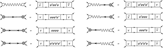
In the definitions above, the particle-particle () and particle-hole () correlation functions defined by Eqs. (9,10) are employed, while the mappings of Eqs. (36,39) to the particle-vibration coupling (PVC) are displayed diagrammatically in Fig. 1.
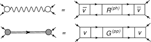

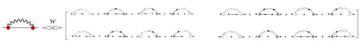
Thus, Eq. (32) is the foundation for microscopic approaches to the single-particle self-energy, which refer to the phenomenon of PVC. The mappings (36,39) lead to the diagrammatic form of the self-energy shown in Fig. 2. The spectral representations of the respective terms read:
| (42) |
| (43) |
| (44) | |||||
Here the single-particle energies in the neighboring -particle system are defined as and those in the -particle system as .
The complete dynamical part (32-35) of the fermionic self-energy truncated at the two-body level is shown in Fig. 2 in the diagrammatic form. Note that the signs in front of the diagrams are convention dependent, for instance, they may not respect Feynman’s convention. For instance, the last uncorrelated term is often shown with the ”-” sign in the literature, and the phonon vertices may include the multiplier ””. The first two diagrams on the right-hand side in Fig. 2 are the typical one-loop diagrams, which are analogous to the electron self-energy correction in quantum electrodynamics (QED). In electronic systems, an electron typically emits and reabsorbs a virtual photon or a phonon excitation of the lattice in a metal. In the nucleonic self-energy of quantum hadrodynamics (QHD) a single nucleon emits and reabsorbs mesons of various kinds, which in the lowest order can be described by the first diagram on the right-hand side if the wavy line is attributed to the meson propagator. In the applications discussed in this work, the meson exchange acts as a bare interaction (although slightly renormalized) described by the matrix elements of . The dynamical self-energy then expresses the medium-induced emerging contribution to the fermionic interaction. Quite remarkably, in the leading approximation dominated by the term (42) in a strong coupling regime, the dynamical fermionic self-energy takes an analogous form of the boson exchange, thereby illustrating how this type of interaction is driven across the energy scales. This process can be expressed by an effective Hamiltonian with the explicit phonon degrees of freedom, as it is done in the phenomenological NFT. The difference between the nuclear system and QED or QHD, besides the differences in the reference (”vacuum”) states, is that in the latter theories, the fermionic and bosonic degrees of freedom are independent. Interestingly, the PVC vertices in nuclear systems are not the effective parameters of the theory but are in principle calculable from the underlying fermionic bare interaction.
There are very few realizations of the PVC model based on the bare NN interaction Barbieri and Hjorth-Jensen (2009); Barbieri (2009). The implementations employing effective interactions Litvinova and Ring (2006); Litvinova (2012); Litvinova and Afanasjev (2011); Afanasjev and Litvinova (2015) are more accurate quantitatively and more feasible because the phonons can be reasonably described already on the level of (quasiparticle) random phase approximation ((Q)RPA) and successive iterations of the fermionic propagator in the Dyson equation may be omitted. However, such approaches inevitably imply an additional procedure to remove the double counting of PVC, implicitly contained in the effective interaction Tselyaev (2013). An elegant way of avoiding such double counting is the explicit subtraction of the dynamical PVC kernel taken in the static limit from the effective interaction. The subtraction method is widely applied in calculations of two-nucleon Green functions, in particular, the particle-hole response Tselyaev (2013); Litvinova and Tselyaev (2007); Litvinova et al. (2007a, 2008); Gambacurta et al. (2015); Litvinova and Schuck (2019), while a corresponding method has not been yet adopted to the case of the one-body propagator.
The information about the two-fermion propagators and in terms of the phonon vertices and propagators can be obtained from their direct computation by solving the EOMs for these correlation functions. The theory and implementations of the corresponding EOMs are presented in Refs. Dukelsky et al. (1998); Olevano et al. (2018); Litvinova and Schuck (2019, 2020).
The spectral forms (42-44) of the three terms with the explicit locality and unitarity are best suited for the accurate diagrammatic mapping and they reveal a different sign of the ”second-order” term as compared to the ”radiative correction” terms and containing phonons. This means, in particular, that potentially the positivity can be violated in the optical theorem. As it was pointed out, for instance, in Refs. Schuck et al. (1973); Danielewicz and Schuck (1994), to prevent this violation it is important to keep the integrity of the spectral representation of the dynamical self-energy (LABEL:Tr)
Comparing the exact dynamical self-energy of Eq. (LABEL:pphgfspec) to Eqs. (42-44), one can see clearly that the above-mentioned sign problem and potentially other inconsistencies may appear because of the different analytical structures of the exact and approximate solutions.
One may notice that the poles of the in Eq. (LABEL:pphgfspec) coincide with those of the one-fermion propagator in the form of Eq. (7), because both sums on the right-hand sides of these expressions run over the complete formally exact spectra of the same systems. Combining these equations with Eq. (23) and considering the energy argument close to the exact pole , one obtains:
| (46) |
which is consistent with the exact EOM for a single field operator Zelevinsky and Volya (2017).
Considerable effort on finding viable approximations for the irreducible part of compatible with the spectral expansion (LABEL:pphgfspec) was undertaken in the past. The authors of Ref. Schuck et al. (1973) have formulated the two-particle-one-hole () RPA for this correlation function, while a more accurate approximation to the energies and matrix elements via Faddeev series has been developed in Ref. Danielewicz and Schuck (1994) to include emergent collectivity in the and channels. Nuclear structure implementations, however, are still quite limited and confined by the Tamm-Dancoff and random phase approximations to the and correlation functions Rijsdijk et al. (1992, 1996); Barbieri and Hjorth-Jensen (2009); Barbieri (2009).
II.3 Superfluid phase
The majority of strongly-correlated fermionic systems, including atomic nuclei, exhibit pronounced effects of superfluidity Ring and Schuck (1980), that need an extended treatment. The superfluid phase is generally characterized by the enhanced formation of Cooper pairs and pairing phonons, which appear to be a dynamical counterpart of the Cooper pairs. In calculations for normal systems within the PVC approach to the self-energy using effective interactions one usually neglects the pairing phonons because of their relatively low importance, but they should be kept for superfluid systems and also if a bare interaction is used.
Within the PVC approach discussed above the pairing interaction is fully dynamical and mediated by the pairing phonons emerging naturally in the one-fermion self-energy. In the traditional frameworks based on effective interactions, however, the pairing is included in the static approximations, such as the BCS or the Hartree-(Fock)-Bogoliubov (HFB) ones. On this level of description, the corresponding Green function technique is the Gor’kov Green functions, which extends the notion of the one-fermion propagator (6) by introducing anomalous propagators with the same kind of fermionic operators, see Eq. (67) below. These correlation functions do not vanish because correlated fermionic pairs are present in the ground state of the system.
The simplest approach to the Gor’kov Green functions can be obtained from the EOM1 if the two-body correlations are neglected, see, for instance, Gorkov (1958). In ref. Litvinova and Zhang (2021) it is shown how the Gor’kov theory is generalized beyond this approximation, in particular, to the inclusion of the PVC effects in the dynamical self-energy. It is convenient to introduce the HFB basis, or the basis of the Bogoliubov quasiparticles Bogolubov (1947). The states in this basis combine particle and hole states, i.e., the states above and below the Fermi energy:
| (47) |
Here and henceforth the Greek indices are used to denote fermionic states in the HFB basis, while the number indices and the Roman indices are reserved for the single-particle mean-field basis states. The repeated indices imply summation, so that Eq. (47) can be expressed in a matrix form:
| (52) |
where
| (57) |
are unitary matrices. The quasiparticle operators and obey the same anticommutator algebra as the particle operators and , while the matrices and satisfy:
| (58) |
The generalized fermionic propagator, therefore, takes the form
| (61) | |||
| (64) | |||
| (67) |
with
| (68) |
In Ref. Litvinova and Zhang (2021) it was shown in detail how the procedure of generating the one-fermion EOM is performed for all the components of the propagator (67). A unified EOM was obtained, in particular, by transforming the matrix equation for the to the quasiparticle basis. The resulting Gor’kov-Dyson equation for the quasiparticle propagator in the energy domain reads:
| (69) |
The indices and are introduced for the quasiparticle forward and backward components, respectively. The mean-field and exact propagator components are defined as follows:
| (70) |
| (71) |
with the mean-field energies of the Bogoliubov quasiparticles and formally exact quasiparticle energies . The residues are the matrix element products and with the formally exact states and . The components of the dynamical kernel in the quasiparticle basis are related to those in the single-particle basis as follows:
| (77) |
| (83) |
while the matrix structure of the dynamical self-energy corresponds to the structure of the propagator matrix (67):
| (84) |
The components of the exact dynamical self-energy are obtainable as the Fourier images of the double contractions of the three-fermion correlators with two interaction matrix elements:
In analogy to the normal case, the components (LABEL:Tsfdyn) of the superfluid dynamical kernel can be treated in various approximations. In particular, one can apply the general cluster decomposition (31) to each of these components. However, in the superfluid ground state, more correlation functions will give non-vanishing contributions. As mentioned above, the approximation, where the many-body problem is truncated on the two-body level, i.e., the PVC approximation and its variants, is the most important one for applications to the regimes of intermediate coupling as it enables a good compromise between accuracy and feasibility. In the extension of the PVC approach to the superfluid, or quasiparticle, PVC dubbed as qPVC, the one-fermion propagators extend to the Gor’kov Green functions (67), and the two-fermion propagators include the contributions collected in Fig. 3 in the diagrammatic representation.
After the corresponding algebra discussed in detail in Ref. Litvinova and Zhang (2021), in the qPVC approach the dynamical kernel takes the form
| (86) |
where the vertex functions and are defined as follows:
| (87) | |||
| (88) |
The component of has an analogous form, however, in practice the equation of the set (69) is redundant as it has the same solution as its counterpart. In the leading approximation, i.e., with the HFB values for the matrix elements and , Eqs. (87,88) reduce to
| (89) |
| (90) |
In this way, one arrives at the compact form of the Gor’kov-Dyson equation (69) in the qPVC approximation, where the dynamical kernel (86) has essentially the same form as in the non-superfluid case. The corresponding operation is shown in Fig. 4. All the complexity arising from the superfluidity is thus transferred to the qPVC vertices (87,88). Essentially, in this framework both the normal and pairing phonons are unified in the superfluid phonons, whose vertices can be linked to the variations of the Hamiltonian of the Bogoliubov quasiparticles Litvinova and Zhang (2021).
II.4 Response theory
The EOMs for the two-fermion propagators defined by Eqs. (9,10) were obtained, for instance, in Refs. Adachi and Schuck (1989); Dukelsky et al. (1998) and, particularly, the PVC approximation was discussed in Refs. Litvinova and Schuck (2019); Schuck (2019); Litvinova and Schuck (2020). The direct ”superfluid” generalization of Eqs. (9,10) unifies these propagators, however, working in terms of Gor’kov Green functions (67) is quite cumbersome because of the quickly increasing number of components. It turns out that the formalism becomes more accessible if the EOM is derived in the quasiparticle space (47) from the beginning. While the detailed derivation was presented in Ref. Litvinova and Zhang (2022), here we concentrate on the major building blocks of the general theory and concrete feasible approximations.
In the quasiparticle basis, the Hamiltonian (1) takes the following form Ring and Schuck (1980):
| (91) | |||||
The upper indices in the matrix elements and are associated with the numbers of creation and annihilation quasiparticle operators in the associated terms. The matrix elements are listed, for instance, in Ring and Schuck (1980). The matrix vanishes at the stationary point defining the HFB equations, while the matrix elements of correspond to the quasiparticle energies. Thus, with , the Hamiltonian reads Ring and Schuck (1980):
| (92) |
where includes the remaining terms and has the meaning of the residual interaction:
| (93) | |||||
The definition of the superfluid response function to a sufficiently weak external field can be deduced from the generic strength function:
| (94) |
where the summation runs over all the formally exact excited states . The generic one-body operator in terms of the quasiparticle fields reads:
| (95) |
following Bogolyubov’s transformation of the second-quantized form of . The full composition in the quasiparticle basis contains formally also terms, however, their contribution vanishes in the leading approximations to the superfluid response Avogadro and Nakatsukasa (2011). Subleading contributions will be considered elsewhere. Eq. (94) can be transformed as follows:
| (100) |
where the matrix of the response function reads:
| (105) | |||
| (109) | |||
| (110) |
with the matrix elements
| (111) |
In terms of the time-dependent field operators, it can be thus defined as
| (114) | |||
| (117) | |||
| (118) |
where we introduce the time-dependent operator products in the Heisenberg picture:
| (119) |
The EOM for the superfluid response (118) is generated by the same technique. Differentiating Eq. (118) sequentially with respect to and and performing the Fourier transformation, one obtains
| (120) |
which has the form of the Bethe-Salpeter-Dyson equation, but with the matrix structure in the quasiparticle basis. The free response is meanwhile defined as
| (121) |
with
| (122) |
and the norm matrix specified below. The interaction kernel is given by
| (123) |
with the static and dynamical -matrices in the quasiparticle space:
| (124) |
| (127) | |||
| (128) |
The norm matrix also acquires an extended form and reads:
| (129) |
with the inverse introduced according to the identity:
So far the theory is still very general and, in order to proceed, evaluation of the double commutators of Eq. (124) and the commutator products of Eq. (128) is required. The ab-initio form of the static kernel (124) is the unification of the and static kernels discussed in Refs. Schuck and Tohyama (2016b); Litvinova and Schuck (2019); Schuck (2019); Litvinova and Schuck (2020); Schuck et al. (2021). In addition to the pure contributions from the bare fermionic interaction, these kernels contain the terms with contractions of the interaction with the correlated parts of the two-body fermionic densities. The latter should be generalized to the superfluid two-body densities and include feedback from the dynamical kernel, which will be considered elsewhere. If the ground state is confined by the HFB approximation, the superfluid static kernel simplifies to the well-known kernel of the quasiparticle random phase approximation (QRPA), with the expectation values of the commutators
| (131) | |||||
while the remaining matrix elements of Eq. (124) can be obtained by Hermitian conjugation.
The components of the dynamical kernel defined by the time-dependent commutator products of Eq. (128) can be evaluated similarly. The diagonal components provide the dominant contribution, while the non-diagonal ones contribute via complex ground-state correlations. The latter will be neglected in this work. Furthermore, the diagonal components are connected by the relationship
| (132) |
so that it is sufficient to explicitly obtain . Its -matrix counterpart
| (133) |
generates a product of eight quasiparticle operators, four at time and four at time , i.e., fully correlated two-times four-quasiparticle propagator, contracted with two matrix elements of the residual interaction. The appearance of such a propagator in the dynamical kernel signals about generating of a hierarchy of coupled EOMs for growing-rank propagators also in the two-fermionic sector. Again, various approximations of increasing accuracy constructed by a factorization procedure are possible, and here we narrow the discussion to the factorizations, which keep all the possible contributions with two-fermion propagators (118). After dropping the complex ground state correlation contributions, the component takes the form
| (134) | |||||
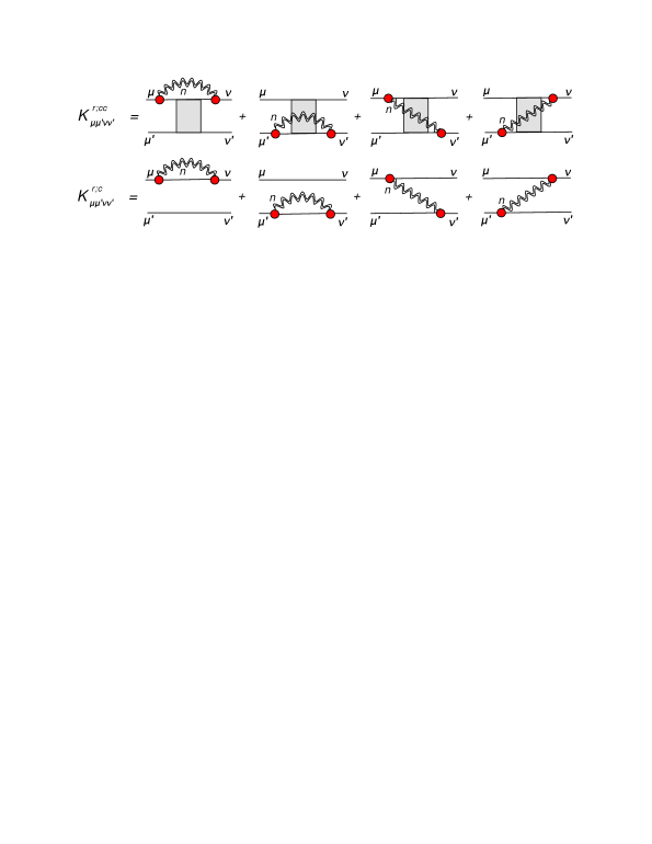
where includes all the antisymmetrizations and the additional upper index ”cc” indicates the approximation, where two fully correlated two-fermion propagators are retained. The diagrammatic interpretation of Eq. (134) is illustrated in Fig. 5. One can notice that, although two two-fermion CFs are figuring in this kernel, only one of them forms a phonon, because only two matrix elements of the NN interaction are entering the initial expression (128), and thus only one CF contracted with these matrix elements can be mapped to the PVC according to Eqs. (36,39). This is at variance with the QPM, see, for instance, the QPM kernels analyzed in Ref. Malov et al. (1985), which contain the two-phonon and, in principle, further multiphonon contributions. These contributions are practically postulated in the ansatz of the excited state wave function, whose coefficients are then found variationally. It is not straightforwardly clear, therefore, if the -phonon QPM with can be obtained as a cluster approximation to the dynamical kernel (128). This may be possible in further approximation to the phonons where they are confined by the (Q)RPA as, in this case, the quasiparticle pair operators can be expressed via the phonon operators; however, we leave this as a conjecture here for a future more accurate investigation.
We note also that the two-quasiparticle CFs and phonons appearing in the dynamical kernel (134) are formally exact and, therefore, are not associated with any partial resummations or perturbative expansions. This indicates that the cluster approaches discussed in this section can include arbitrarily complex 2n-quasiparticle configurations. However, approximations can always be applied to calculations of the phonons.
Finally, by relaxing the correlations in the intermediate two-quasiparticle propagator, which is not associated with a phonon, in Eq. (134), one obtains its qPVC-NFT approximation:
| (135) |
where we indicated by the index ”c” that only one two-quasiparticle correlation function is retained in the dynamical kernel. To bring this kernel to the form, which corresponds to the superfluid generalization of the NFT, one can recast Eq. (135) by performing the explicit antisymmetrizations and rearranging the resulting terms as follows:
| (136) |
This form of the dynamical kernel can be further simplified if the pairing correlations are approximated by the BCS theory, see for instance, Ref. Zelevinsky and Volya (2017). It is essentially an analog of the resonant kernel obtained in phenomenological approaches of the NFT Niu et al. (2016) and quasiparticle time blocking approximation Tselyaev (2007); Litvinova and Tselyaev (2007). Finally, we note that on the way to Eqs. (134-136) a number of correlations were neglected in the versions and of the kernel, which are considered to be the leading, sometimes called resonant, approximations. The major subleading contributions are then associated with the amplitudes, the terms of the residual interaction other than , and the off-diagonal and contributions. They can be straightforwardly included due to the universality and completeness of the presented framework, which thus offers a number of extensions beyond the qPVC approaches and given explicitly in this section.
II.5 Self-consistent implementations of the qPVC approaches for nuclear response
The simplest resonant qPVC dynamical kernel has been a subject of self-consistent implementations based on the effective in-medium NN interactions derived from the DFT. The applications to the nuclear response include, for instance, the ones with the zero-range phenomenological Skyrme interaction Tselyaev et al. (2018); Lyutorovich et al. (2018); Niu et al. (2016, 2018). The self-consistency in this context means that (i) the static kernels of the one-fermion and two-fermion EOMs are approximated by the first and second variational derivatives of the EDF, respectively, (ii) the phonons’ characteristics are obtained with the same interaction, and (iii) the subtraction of the static limit of the dynamical kernel Tselyaev (2013) is applied to eliminate the double counting of its admixture to the effective interaction.
The fully self-consistent qPVC approaches to the nuclear response with the more fundamental background of the relativistic meson-nucleon Lagrangian are available since Ref. Litvinova et al. (2008) under the relativistic time blocking approximation (RQTBA) in the more general context of the relativistic nuclear field theory (RNFT) and include calculations for both the neutral Litvinova et al. (2009a, 2010); Endres et al. (2010); Massarczyk et al. (2012); Lanza et al. (2014); Poltoratska et al. (2014); Negi et al. (2016); Egorova and Litvinova (2016); Carter et al. (2022); Litvinova (2023) and charge-exchange Robin and Litvinova (2016); Scott et al. (2017); Robin and Litvinova (2018, 2019) excitations. Important improvements due to the inclusion of the qPVC dynamical kernel have been found already in the leading approximation (136). The widths of the giant resonances, the isospin character of the low-energy soft modes and overall strength distributions, beta decay, nuclear compressibility, and other nuclear structure properties were described in a single framework with universal parameters across the nuclear chart. The complete self-consistency, the covariant nature of the RNFT, and its background in the microscopic NN interaction, only slightly adjusted to the nuclear medium, provide a good balance of fundamentality and accuracy, making this theory most predictive, transferrable across the energy scales and systematically improvable. The latter two features were enabled after the recent completion of the ab-initio EOM qPVC framework Litvinova and Schuck (2019, 2020); Litvinova and Zhang (2021, 2022) outlined in the previous sections. Other recent developments extend the RNFT to finite temperature Litvinova and Wibowo (2018, 2019); Litvinova et al. (2020); Litvinova and Robin (2021), making it the theory of choice for predictive astrophysical applications, and include correlations of higher complexity, Litvinova (2015); Robin and Litvinova (2019); Litvinova and Schuck (2019), heading toward spectroscopically accurate calculations in large model spaces.
As the time blocking Tselyaev (2007) applied to the four-point correlation functions is not needed for the two-point response, the qPVC approaches presented in this work are dubbed as relativistic EOM (REOMn) with the upper index indicating the maximal configuration complexity of the dynamical kernel.
III Nuclear response in RNFT framework
The response function is commonly actualized via its convolution with the operators, which are associated with external probes of the system under study. The resulting quantity which describes the observed spectra is the strength function, which for the given external field operator can be expressed as
| (137) |
while its form in the quasiparticle basis is given in subsection II.4. In this work, we consider the response to the electromagnetic dipole and quadrupole operators, respectively,
| (138) |
where and are the numbers of protons and neutrons, respectively, , and is the proton charge, which is taken . The sums in Eq. (138) are performed over the corresponding nucleonic degrees of freedom.
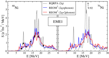
Figs. 6 and 7 illustrate the RNFT calculations of the dipole response of the two neutron-rich nickel isotopes 68,70Ni. The theoretical results are obtained in the three relativistic approaches: (i) Relativistic QRPA (RQRPA) Paar et al. (2003) confined by the configurations, (ii) relativistic EOM confined by correlated , or four-quasiparticle, configurations , employing the dynamical kernel (136) illustrated in the lower part of Fig. 5 and dubbed as REOM2, and (iii) relativistic EOM confined by correlated , or six-quasiparticle, configurations , employing the dynamical kernel (134) illustrated in the upper part of Fig. 5 and dubbed as REOM3. In the latter approximation, the configuration complexity is achieved by recycling the correlated propagators in the kernel of Eq. (134). The following multi-step calculation scheme is implemented:
-
•
The closed set of the relativistic mean field (RMF) Hartree-Bogoliubov equations Serot and Walecka (1986); Ring (1996); Vretenar et al. (2005) is solved with the NL3 effective interaction following Refs. Boguta and Bodmer (1977); Lalazissis et al. (1997), with the monopole pairing forces adjusted to reproduce empirical pairing gaps. The resulting single-particle Dirac spinors and single-nucleon energies form the working basis for subsequent calculations. No further parameters are introduced.
-
•
The RQRPA equation Paar et al. (2003), which is equivalent to Eq. (120) with the only static kernel (124) approximated by Eqs. (131) with the effective interaction matrix elements, is solved to obtain the phonon vertices and their frequencies . The phonons with the = 2+, 3-, 4+, 5-, 6+ and frequencies 15 MeV coupled to the RMF quasiparticle states form the configuration space for the qPVC kernels. The phonon space was additionally truncated: the modes with the values of the reduced transition probabilities less than 5% of the maximal one (for each ) were neglected. These are the common truncation criteria for the qPVC models based on the RMF, see, for instance, Litvinova (2016), where a convergence study was presented. The convergence is further reinforced by the subtraction procedure Tselyaev (2013).
-
•
Additional step for the REOM 3 approach: Eq. (120) for the response function is solved in the truncated configuration space, which includes excitations within the energy window of interest 0-25 MeV, for spins and parities = 0± - 6±. As in Ref. Litvinova and Schuck (2019), the static part of the kernel is neglected in the internal correlation functions as it does not induce fragmentation. The resulting response functions are inserted into the kernel (134).
- •
-
•
Finally, the strength functions are found according to Eq. (LABEL:Polar).
Further details of the calculation scheme can be found in Ref. Litvinova and Schuck (2019), where the REOM3 was presented for the first time and applied to the dipole response of calcium isotopes. Here we focus on the dipole transitions of the neutron-rich unstable nickel isotopes, which are extensively studied both theoretically and experimentally and which are of special significance for astrophysics.
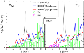
In the left panel of Fig. 6 the dipole strength distributions in 68Ni obtained in the three approaches with the same parameter set and with keV illustrate the hierarchy of approximations of growing complexity. Experimental data from Ref. Rossi et al. (2013) are plotted for comparison after scaling to accommodate the enhancement of the Thomas-Reiche-Kuhn sum rule. Remarkably, the REOM2, which includes the leading effects of emergent collectivity, provides a major improvement of the description. The REOM3 including more complex qPVC correlations in the dynamical kernel further refines the strength distribution, but the overall effect on the smeared strength is less drastic. Similar results are obtained for 70Ni, for which the experimental data are available only at low energies, see Fig. 7 and discussion below.
Calculations in the REOM3 approach are significantly heavier than those in REOM2 because a large, ideally complete, set of the internal CFs enters the doubly correlated kernel of REOM3. The set of phonons coupled to those CFs in the kernel of Eq. (134) is also formally complete, however, the CFs in the phonons enter in the form of contraction with the interaction matrix elements, i.e., with the phonons’ vertices . As it follows from numerous previous RQTBA studies, these vertices behave as emergent order parameters, which enables reasonably accurate truncation schemes of the phonon model subspaces. Moreover, as the most significant phonons are well reproduced within RQRPA, reiterating their CFs does not bring significant improvements. However, reiterating and keeping a sufficiently complete set of the internal non-contracted CFs appears to be quantitatively important. This is the major factor that makes large-scale studies difficult, however, simple parallelization algorithms can be implemented to improve the time scaling of the REOM3 approach.
The cases of 68,70Ni can be compared to those of 42,48Ca presented in Ref. Litvinova and Schuck (2019). Similarly, configurations included in REOM3 induce a stronger fragmentation of the GDR and its additional spreading toward both higher and lower energies. Visible shifts of the main peaks of the giant dipole resonance (GDR) toward higher energies were obtained in 42,48Ca due to these high-complexity configurations. This observation was related to the appearance of the new higher-energy complex configurations and, consequently, the additional higher-energy poles in the resulting response functions. However, it was unclear whether or not the shift of the main peak is a generic feature of the configurations. The results for the 68,70Ni isotopes indicate that this effect is selective as no pronounced shifts are observed. As noted in Litvinova and Schuck (2019), the energy-weighted sum rule is conserved in REOM3 because the analytical form of its dynamical kernel does not change as compared to REOM2.
The low-energy dipole response of the unstable neutron-rich 68,70Ni nuclei is of special significance as they are located on the r-process nucleosynthesis path. Because of its relevance to astrophysics, it has been investigated both experimentally Wieland et al. (2009); Rossi et al. (2013); Wieland et al. (2018) and theoretically Litvinova et al. (2010, 2013); Papakonstantinou et al. (2015). The results of the RQRPA, REOM2 and REOM3 calculations for the low-energy dipole response of 68,70Ni are displayed in Fig. 7 with the same curve and color-coding as in Fig. 6. In particular, one can see how richer spectra of REOM2 and REOM3 emerge from a relatively poor one of RQRPA. The latter is essentially the single strong and relatively collective state at MeV in both nuclei with more strength in the case of 70Ni because of its larger neutron excess. The addition of configurations of REOM2 results in the fragmentation of this state over a broader energy region. Finally, with the configurations, the fragmentation effect is further reinforced resulting in a distribution without a clear dominance of a single state but is rather spread uniformly over the MeV energy interval with a smooth strength increase toward the GDR. One can notice also the appearance of excited states at lower energies. Thus, these examples illustrate how the three models with the increasing complexity of the dynamical kernel form a hierarchy that translates to the hierarchy of spectral functions with the increasing richness of their fine structure. The results in this energy region are compared to experimental data of Ref. Wieland et al. (2018), where the two parts of the strength distribution in 70Ni were obtained by different methods, that are indicated by different colors. One can see that a sequential increase of configuration complexity in the response theory improves the description, while the highest-complexity configurations still bring significant changes to the low-energy spectra. This suggests that such configurations are important for the quantities, which are sensitive to the details of the low-energy strength distributions, in particular, the radiative neutron capture rates in the r-process. Similar effects for the isospin-flip transitions and thus further refinements of the beta decay rates as compared to, e.g., Refs. Robin and Litvinova (2016); Litvinova et al. (2020) are expected.
The low-energy dipole strength, associated with the neutron skin oscillation and also known as pygmy dipole resonance (PDR), attracts active attention from both theory and experiment Savran et al. (2013); Lanza et al. (2023). Its fine structure and relevance for astrophysics were addressed in numerous RNFT studies Litvinova et al. (2007b, 2009b, 2009a); Endres et al. (2010); Massarczyk et al. (2012); Litvinova and Belov (2013); Poltoratska et al. (2014); Özel-Tashenov et al. (2014); Lanza et al. (2014); Negi et al. (2016). The detailed knowledge on the low-energy strength of quadrupole character is limited, but also represents an interesting subject Tsoneva and Lenske (2011); Spieker et al. (2016); Tsoneva et al. (2019); Lenske and Tsoneva (2019). In particular, in Ref. Tsoneva and Lenske (2011) the electric quadrupole response was investigated theoretically within the QPM along the Sn isotopic chain with special emphasis on excitations above the first collective state and below the particle emission threshold. This study has reported that depending on the asymmetry, a quadrupole strength clustering similar to the known PDR is found. The authors concluded from analyzing the transition densities of low-energy quadrupole states that the obtained results are compatible with oscillations of neutron or proton skins against the isospin-saturated core and with experimental data Spieker et al. (2016); Tsoneva et al. (2019).
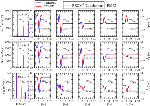
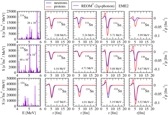
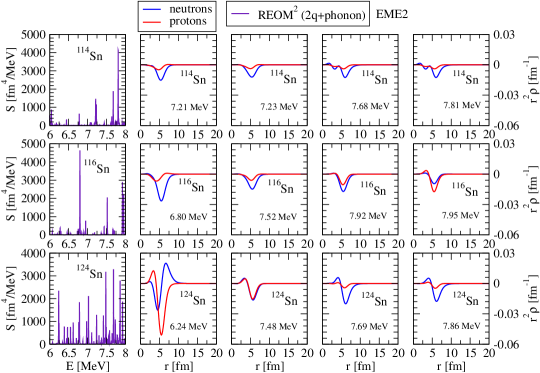
Figs. 8 - 10 demonstrates the capability of RNFT to describe the quadrupole strength displaying the REOM2 results for the 2+ electromagnetic (EME2) excitations in three even-even tin isotopes 114,116,124Sn below 8 MeV, i.e., below their particle emission thresholds (10.3, 9.6, and 8.5 MeV, respectively). From the long tin isotopic chain, the 114,116Sn isotopes were selected for this study as the two typical mid-shell nuclei with similar moderate neutron excess, to investigate how the minimal difference in the neutron number translated to the differences and similarities in their 2+ strength distributions. The 124Sn was chosen as the isotope with a significantly larger neutron number, potentially forming a prominent neutron skin. The structure of the quadrupole spectra in the considered energy region is qualitatively similar in all three nuclei: there is a strong collective lowest state at around 1 MeV and a group of states at higher energies with varying strength. The giant quadrupole resonance in these nuclei is located above 20 MeV and is not examined here. The RQRPA results for the lowest collective 2+ state are given and discussed in Ref. Afanasjev and Litvinova (2015). The major effect of adding configurations on this state is a minor downward shift, which brings its position closer to the experimental values, and a slight reduction of the transition probability. In the studies of Refs. Tsoneva and Lenske (2011); Spieker et al. (2016); Tsoneva et al. (2019) the lowest 2+ state is interpreted as a phenomenon, which is structurally separated from the other quadrupole excitations at higher energies, while the latter ones were associated with pygmy quadrupole resonance.
The REOM2 EME2 spectra in 114,116,124Sn below 4 MeV is shown in the left panels of Fig. 8, while the transition densities of the most pronounced excited states are given on the right-hand side of the respective strength distributions. The latter is calculated with a small value of the smearing parameter keV to resolve the fine structure of the strength. The reduced transition probabilities can be related to the values of the strength functions at the peaks at as . The transition densities of the lowest 2+ state are prevailed by the in-phase surface oscillation of the neutron and proton Fermi liquids with some neutron dominance and in the case of 114,116Sn show out-of-phase overtones in the bulk. While moving toward the upper bound of the MeV energy interval, the next general trend is the weakening of the surface oscillations, which remain in phase, and the reduction of the neutron dominance. The next part of the spectrum illustrated in Fig. 9 in the same manner shows a significant increase of the density of states. The trends in the behavior of the transition densities of the strongest 2+ excitations change showing the growth of the surface oscillation amplitudes and, interestingly, a proton dominance in all the nuclei for the majority of states in the MeV energy interval. When moving beyond this energy interval, the density of states further increases and the transition densities change back to mainly neutron-dominant character, except for one state at E = 6.24 MeV in 124Sn. The reduction of amplitudes of the oscillations reflects stronger qPVC effects in the formation of the corresponding states in the MeV energy interval as the qPVC takes away considerable parts of the total normalization of the transition densities Litvinova et al. (2007a). Some enhancement in the surface oscillation intensity is noted in 124Sn that can be attributed to its neutron richness. At variance with Refs. Spieker et al. (2016); Lenske and Tsoneva (2019), REOM2 calculations do not show a dominance of out-of-phase oscillations of neutrons vs protons below 5 MeV. However, the transition densities for the 2+ state at E = 6.24 MeV in 124Sn indicate that such oscillations can be present in the energy region under study. The near absence of such states, which are typical for the energies between the PDR and GDR, is consistent with the fact that the giant quadrupole resonance represents a oscillation mode and therefore is located at a much higher energy than the GDR. This means, in particular, that the ”pygmy quadrupole” mode may be spread over a wider energy interval toward higher energy, which calls for further detailed studies of this phenomenon.
IV Summary
A theoretical framework for the low-rank fermionic propagators, most relevant to the observables in strongly-coupled superfluid fermionic many-body systems, is presented. The equations of motion for the two-times one-fermion and two-fermion superfluid propagators are obtained continuously with the only input of the bare two-fermion interaction. The EOM for the one-fermion propagator is worked out in the single-particle space and shown to simplify after the transformation to the HFB basis. This operation reveals important relationships between the two representations, scales the computational effort down considerably for realistic implementations, and paves the way to the superfluid response theory, which is obtained in the HFB basis from the start.
The exact forms of the interaction kernels containing higher-rank propagators in their dynamical components are discussed. These propagators are approximated by factorizations into the possible products of two-fermion and one-fermion propagators in the superfluid regime, thereby introducing the truncation of the many-body problem on the two-body level, keeping the leading effects of emergent collectivity. It is thus and further shown how, with gradually relaxing correlations, the exact theory is reduced to the known approximations.
The major focus is then directed on the quasiparticle-vibration coupling in the dynamical kernels, where the normal and pairing phonons become components of the unified superfluid phonons. Self-consistent implementations are presented in the framework of the relativistic nuclear field theory for the dipole and quadrupole responses of the neutron-rich nickel and tin isotopes, respectively. The analysis of the obtained results is concentrated on the qPVC effects, which considerably modify the strength distributions, introducing their fragmentation and shifting the positions of the major peaks. Comparison of the strength distributions for the electromagnetic dipole response in 68,70Ni computed with configurations up to with experimental data indicates that increasing the configuration complexity of the dynamical kernel brings the theoretical results in better agreement with the data. At the same time, the resulting strength functions show saturation of its general features, so that the higher-complexity configurations may appear to be more important for the fine structure of the obtained spectra than for their gross structure. A study of the low-energy electromagnetic quadrupole strength was performed for the first time within the RNFT response theory confined by configurations for 114,116,124Sn and revealed some new insights in the underlying structure of the individual states forming this strength. The obtained results accentuate the importance of further advancing the quantum many-body theory in the sector of complex configurations which, in turn, give feedback on the static kernels of the fermionic EOMs. Addressing the latter aspect of the many-body problem is also necessary for heading toward spectroscopically accurate nuclear theory respecting special relativity and rooted in the standard model of particle physics.
Acknowledgement
Illuminating discussions with Mark Spieker, Nadezhda Tsoneva, Enrico Vigezzi, and Horst Lenske are gratefully acknowledged. This work was supported by the GANIL Visitor Program, US-NSF Grant PHY-2209376, and US-NSF Career Grant PHY-1654379.
References
- Matsubara (1955) T. Matsubara, Progress in Theoretical Physics 14 (1955).
- Watson (1956) K. M. Watson, Physical Review 103, 489 (1956).
- Brueckner and Levinson (1955) K. A. Brueckner and C. A. Levinson, Physical Review 97, 1344 (1955).
- Brueckner (1955) K. A. Brueckner, Physical Review 100, 36 (1955).
- Martin and Schwinger (1959) P. C. Martin and J. S. Schwinger, Physical Review 115, 1342 (1959).
- Ethofer (1969) S. Ethofer, Zeitschrift für Physik A 225, 353 (1969).
- Schuck and Ethofer (1973) P. Schuck and S. Ethofer, Nuclear Physics A212, 269 (1973).
- Gorkov (1958) L. P. Gorkov, Soviet Physics JETP 7, 505 (1958).
- Kadanoff and Martin (1961) L. P. Kadanoff and P. C. Martin, Physical Review 124, 670 (1961).
- Ethofer and Schuck (1969) S. Ethofer and P. Schuck, Zeitschrift für Physik 228, 264 (1969).
- Rowe (1968) D. J. Rowe, Review of Modern Physics 40, 153 (1968).
- Schuck (1976) P. Schuck, Zeitschrift für Physik A 279, 31 (1976).
- Adachi and Schuck (1989) S. Adachi and P. Schuck, Nuclear Physics A496, 485 (1989).
- Danielewicz and Schuck (1994) P. Danielewicz and P. Schuck, Nuclear Physics A567, 78 (1994).
- Dukelsky et al. (1998) J. Dukelsky, G. Röpke, and P. Schuck, Nuclear Physics A628, 17 (1998).
- Litvinova and Schuck (2019) E. Litvinova and P. Schuck, Physical Review C 100, 064320 (2019).
- Tiago et al. (2008) M. L. Tiago, P. Kent, R. Q. Hood, and F. A. Reboredo, Journal of Chemical Physics 129, 084311 (2008).
- Martinez et al. (2010) J. I. Martinez, J. García-Lastra, M. López, and J. Alonso, Journal of Chemical Physics 132, 044314 (2010).
- Sangalli et al. (2011) D. Sangalli, P. Romaniello, G. Onida, and A. Marini, Journal of Chemical Physics 134, 034115 (2011).
- Schuck and Tohyama (2016a) P. Schuck and M. Tohyama, European Physical Journal A 52, 307 (2016a).
- Olevano et al. (2018) V. Olevano, J. Toulouse, and P. Schuck, Journal of Chemical Physics 150, 084112 (2018).
- Schuck et al. (2021) P. Schuck, D. Delion, J. Dukelsky, M. Jemai, E. Litvinova, G. Roepke, and M. Tohyama, Physics Reports 929, 1 (2021).
- Schuck (2019) P. Schuck, European Physical Journal A55, 250 (2019).
- Litvinova and Schuck (2020) E. Litvinova and P. Schuck, Physical Review C 102, 034310 (2020).
- Litvinova and Schuck (2021) E. Litvinova and P. Schuck, Physical Review C 104, 044330 (2021).
- Bohr and Mottelson (1969) A. Bohr and B. R. Mottelson, Nuclear structure, Vol. 1 (World Scientific, 1969).
- Bohr and Mottelson (1975) A. Bohr and B. R. Mottelson, Nuclear structure, Vol. 2 (Benjamin, New York, 1975).
- Broglia and Bortignon (1976) R. A. Broglia and P. F. Bortignon, Physics Letters B65, 221 (1976).
- Bortignon et al. (1977) P. F. Bortignon, R. Broglia, D. Bes, and R. Liotta, Physics Reports 30, 305 (1977).
- Bertsch et al. (1983) G. Bertsch, P. Bortignon, and R. Broglia, Reviews of Modern Physics 55, 287 (1983).
- Tselyaev (1989) V. Tselyaev, Soviet Journal of Nuclear Physics 50, 780 (1989).
- Litvinova and Tselyaev (2007) E. Litvinova and V. Tselyaev, Physical Review C 75, 054318 (2007).
- Soloviev (1992) V. Soloviev, Theory of Atomic Nuclei: Quasiparticles and Phonons (Institute of Physics Publishing, 1992).
- Malov and Soloviev (1976) L. A. Malov and V. G. Soloviev, Nuclear Physics A 270, 87 (1976).
- Tselyaev (2013) V. I. Tselyaev, Physical Review C 88, 054301 (2013).
- Litvinova et al. (2007a) E. Litvinova, P. Ring, and V. Tselyaev, Physical Review C 75, 064308 (2007a).
- Litvinova et al. (2008) E. Litvinova, P. Ring, and V. Tselyaev, Physical Review C 78, 014312 (2008).
- Litvinova et al. (2010) E. Litvinova, P. Ring, and V. Tselyaev, Physical Review Letters 105, 022502 (2010).
- Litvinova et al. (2013) E. Litvinova, P. Ring, and V. Tselyaev, Physical Review C 88, 044320 (2013).
- Tselyaev et al. (2018) V. Tselyaev, N. Lyutorovich, J. Speth, and P. G. Reinhard, Physical Review C 97, 044308 (2018).
- Litvinova (2023) E. Litvinova, Physical Review C 107, L041302 (2023).
- Litvinova and Zhang (2021) E. Litvinova and Y. Zhang, Physical Review C 104, 044303 (2021).
- Van der Sluys et al. (1993) V. Van der Sluys, D. Van Neck, M. Waroquier, and J. Ryckebusch, Nuclear Physics A551, 210 (1993).
- Avdeenkov and Kamerdzhiev (1999) A. V. Avdeenkov and S. P. Kamerdzhiev, Physics Letters B459, 423 (1999).
- Avdeenkov and Kamerdzhev (1999) A. V. Avdeenkov and S. P. Kamerdzhev, JETP Letters 69, 715 (1999).
- Barranco et al. (1999) F. Barranco, R. Broglia, G. Gori, E. Vigezzi, P. Bortignon, and J. Terasaki, Physical Review Letters 83, 2147 (1999).
- Barranco et al. (2005) F. Barranco, P. Bortignon, R. Broglia, G. Colò, P. Schuck, E. Vigezzi, and X. Vinas, Physical Review C 72, 054314 (2005).
- Tselyaev (2007) V. I. Tselyaev, Physical Review C 75, 024306 (2007).
- Litvinova and Afanasjev (2011) E. V. Litvinova and A. V. Afanasjev, Physical Review C 84, 014305 (2011).
- Litvinova (2012) E. Litvinova, Physical Review C 85, 021303 (2012).
- Afanasjev and Litvinova (2015) A. V. Afanasjev and E. Litvinova, Physical Review C 92, 044317 (2015).
- Idini et al. (2015) A. Idini, G. Potel, F. Barranco, E. Vigezzi, and R. A. Broglia, Physical Review C 92, 031304 (2015).
- Soma et al. (2011) V. Soma, T. Duguet, and C. Barbieri, Physical Review C 84, 064317 (2011).
- Soma et al. (2013) V. Soma, C. Barbieri, and T. Duguet, Physical Review C 87, 011303 (2013).
- Soma et al. (2014) V. Soma, C. Barbieri, and T. Duguet, Physical Review C 89, 024323 (2014).
- Somà et al. (2021) V. Somà, C. Barbieri, T. Duguet, and P. Navrátil, European Physical Journal A 57, 135 (2021).
- Litvinova and Zhang (2022) E. Litvinova and Y. Zhang, Physical Review C 106, 064316 (2022).
- Gambacurta et al. (2011) D. Gambacurta, M. Grasso, and F. Catara, Physical Review C 84, 034301 (2011).
- Gambacurta et al. (2015) D. Gambacurta, M. Grasso, and J. Engel, Physical Review C 92, 034303 (2015).
- Niu et al. (2014) Y. Niu, G. Colò, and E. Vigezzi, Physical Review C 90, 054328 (2014).
- Niu et al. (2015) Y. Niu, Z. Niu, G. Colò, and E. Vigezzi, Physical Review Letters 114, 142501 (2015).
- Robin and Litvinova (2016) C. Robin and E. Litvinova, European Physical Journal A 52, 205 (2016).
- Robin and Litvinova (2019) C. Robin and E. Litvinova, Physical Review Letters 123, 202501 (2019).
- Ponomarev (1999) V. Yu. Ponomarev, Nucl. Phys. A649, 243 (1999).
- Lo Iudice et al. (2012) N. Lo Iudice, V. Y. Ponomarev, C. Stoyanov, A. V. Sushkov, and V. V. Voronov, Journal of Physics G39, 043101 (2012).
- Savran et al. (2011) D. Savran et al., Phys. Rev. C84, 024326 (2011).
- Tsoneva et al. (2019) N. Tsoneva, M. Spieker, H. Lenske, and A. Zilges, Nuclear Physics A990, 183 (2019).
- Lenske and Tsoneva (2019) H. Lenske and N. Tsoneva, European Physical Journal A 55, 238 (2019).
- Papakonstantinou and Roth (2009) P. Papakonstantinou and R. Roth, Phys. Lett. B 671, 356 (2009).
- Bianco et al. (2012) D. Bianco, F. Knapp, N. Lo Iudice, F. Andreozzi, and A. Porrino, Physical Review C 85, 014313 (2012).
- Bacca et al. (2013) S. Bacca, N. Barnea, G. Hagen, G. Orlandini, and T. Papenbrock, Physical Review Letters 111, 122502 (2013).
- Knapp et al. (2014) F. Knapp, N. Lo Iudice, P. Veselý, F. Andreozzi, G. De Gregorio, and A. Porrino, Physical Review C 90, 014310 (2014).
- Bacca (2014) S. Bacca, Phys. Rev. C 90, 064619 (2014).
- Knapp et al. (2015) F. Knapp, N. Lo Iudice, P. Veselý, F. Andreozzi, G. De Gregorio, and A. Porrino, Physical Review C 92, 054315 (2015).
- De Gregorio et al. (2016a) G. De Gregorio, F. Knapp, N. Lo Iudice, and P. Vesely, Physical Review C 94, 061301(R) (2016a).
- De Gregorio et al. (2016b) G. De Gregorio, F. Knapp, N. Lo Iudice, and P. Vesely, Physical Review C 93, 044314 (2016b).
- Raimondi and Barbieri (2019) F. Raimondi and C. Barbieri, Physical Review C 99, 054327 (2019).
- Brockmann (1978) R. Brockmann, Physical Review C 18, 1510 (1978).
- Boyussy et al. (1987) A. Boyussy, J.-F. Mathiott, N. V. Giai, and S. Marcos, Physical Review C 36, 380 (1987).
- Poschenrieder and Weigel (1988a) P. Poschenrieder and M. K. Weigel, Physics Letters B 200, 231 (1988a).
- Poschenrieder and Weigel (1988b) P. Poschenrieder and M. K. Weigel, Physical Review C 38, 471 (1988b).
- Danielewicz and Namyslowski (1979) P. Danielewicz and J. M. Namyslowski, Physics Letters B 81, 110 (1979).
- Karmanov (2011) V. A. Karmanov, Few Body Systems 50, 61 (2011).
- Dickhoff and Barbieri (2004) W. H. Dickhoff and C. Barbieri, Progress in Particle and Nuclear Physics 52, 377 (2004).
- Dickhoff and Neck (2005) W. H. Dickhoff and D. V. Neck, Many-Body Theory Exposed! (World Scientific, 2005).
- Kucharek and Ring (1991) H. Kucharek and P. Ring, Zeitschrift für Physik A 339, 23 (1991).
- (87) N. Vinh Mau, in Theory of nuclear structure, Trieste Lectures 1069, p. 931 (IAEA, Vienna, 1970).
- Mau and Bouyssy (1976) N. V. Mau and A. Bouyssy, Nuclear Physics A257, 189 (1976).
- Ring and Schuck (1980) P. Ring and P. Schuck, The Nuclear Many-Body Problem (Springer-Verlag Berlin Heidelberg, 1980).
- Rijsdijk et al. (1992) G. A. Rijsdijk, K. Allaart, and W. H. Dickhoff, Nucl. Phys. A 550, 159 (1992).
- Barbieri and Hjorth-Jensen (2009) C. Barbieri and M. Hjorth-Jensen, Physical Review C 79, 064313 (2009).
- Barbieri (2009) C. Barbieri, Physical Review Letters 103, 202502 (2009).
- Litvinova and Ring (2006) E. Litvinova and P. Ring, Physical Review C 73, 044328 (2006).
- Schuck et al. (1973) P. Schuck, F. Villars, and P. Ring, Nuclear Physics A 208, 302 (1973).
- Zelevinsky and Volya (2017) V. Zelevinsky and A. Volya, Physics of Atomic Nuclei (Wiley, 2017).
- Rijsdijk et al. (1996) G. A. Rijsdijk, W. J. W. Geurts, K. Allaart, and W. H. Dickhoff, Physical Review C 53, 201 (1996).
- Bogolubov (1947) N. Bogolubov, Journal of Physics 11, 23 (1947).
- Zhang et al. (2022) Y. Zhang, A. Bjelčić, T. Nikšić, E. Litvinova, P. Ring, and P. Schuck, Physical Review C 105, 044326 (2022).
- Avogadro and Nakatsukasa (2011) P. Avogadro and T. Nakatsukasa, Physical Review C 84, 014314 (2011).
- Schuck and Tohyama (2016b) P. Schuck and M. Tohyama, Physical Review B 93, 165117 (2016b).
- Malov et al. (1985) L. A. Malov, F. M. Meliev, and V. G. Soloviev, Zeitschrift für Physik A 320, 521 (1985).
- Niu et al. (2016) Y. F. Niu, G. Colo, E. Vigezzi, C. L. Bai, and H. Sagawa, Physical Review C 94, 064328 (2016).
- Lyutorovich et al. (2018) N. Lyutorovich, V. Tselyaev, J. Speth, and P. Reinhard, Physical Review C 98, 054304 (2018).
- Niu et al. (2018) Y. Niu, Z. Niu, G. Colò, and E. Vigezzi, Physics Letters B 780, 325 (2018).
- Litvinova et al. (2009a) E. Litvinova, H. Loens, K. Langanke, G. Martinez-Pinedo, T. Rauscher, P. Ring, F.-K. Thielemann, and V. Tselyaev, Nuclear Physics A823, 26 (2009a).
- Endres et al. (2010) J. Endres, E. Litvinova, D. Savran, P. A. Butler, M. N. Harakeh, S. Harissopulos, R.-D. Herzberg, R. Krücken, A. Lagoyannis, N. Pietralla, V. Y. Ponomarev, L. Popescu, P. Ring, M. Scheck, K. Sonnabend, V. I. Stoica, H. J. Wörtche, and A. Zilges, Physical Review Letters 105, 212503 (2010).
- Massarczyk et al. (2012) R. Massarczyk, R. Schwengner, F. Dönau, E. Litvinova, G. Rusev, R. Beyer, R. Hannaske, A. Junghans, M. Kempe, J. H. Kelley, et al., Physical Review C 86, 014319 (2012).
- Lanza et al. (2014) E. Lanza, A. Vitturi, E. Litvinova, and D. Savran, Physical Review C 89, 041601 (2014).
- Poltoratska et al. (2014) I. Poltoratska, R. Fearick, A. Krumbholz, E. Litvinova, H. Matsubara, P. von Neumann-Cosel, V. Y. Ponomarev, A. Richter, and A. Tamii, Physical Review C 89, 054322 (2014).
- Negi et al. (2016) D. Negi, M. Wiedeking, E. G. Lanza, E. Litvinova, A. Vitturi, R. A. Bark, L. A. Bernstein, D. L. Bleuel, D. S. Bvumbi, T. D. Bucher, B. H. Daub, T. S. Dinoko, N. Erasmus, J. L. Easton, A. Görgen, M. Guttormsen, P. Jones, B. V. Kheswa, N. Khumalo8, A. C. Larsen, E. A. Lawrie, J. J. Lawrie, S. N. T. . Majola, L. P. Masiteng, M. R. Nchodu, J. Ndayishimye, R. T. Newman, S. P. Noncolela, J. N. Orce, P. Papka, T. Renstrøm, D. G. Roux, O. Shirinda, S. Siem, P. S. Sithole, and P. C. Uwitonze, Physical Review C 94, 024332 (2016).
- Egorova and Litvinova (2016) I. A. Egorova and E. Litvinova, Physical Review C 94, 034322 (2016).
- Carter et al. (2022) J. Carter et al., Physics Letters B 833, 137374 (2022).
- Scott et al. (2017) M. Scott et al., Physical Review Letters 118, 172501 (2017).
- Robin and Litvinova (2018) C. Robin and E. Litvinova, Physical Review C 98, 051301(R) (2018).
- Litvinova and Wibowo (2018) E. Litvinova and H. Wibowo, Physical Review Letters 121, 082501 (2018).
- Litvinova and Wibowo (2019) E. Litvinova and H. Wibowo, European Physical Journal A55, 223 (2019).
- Litvinova et al. (2020) E. Litvinova, C. Robin, and H. Wibowo, Physics Letters B800, 135134 (2020).
- Litvinova and Robin (2021) E. Litvinova and C. Robin, Physical Review C 103, 024326 (2021).
- Litvinova (2015) E. Litvinova, Physical Review C 91, 034332 (2015).
- Rossi et al. (2013) D. M. Rossi, P. Adrich, F. Aksouh, H. Alvarez-Pol, T. Aumann, J. Benlliure, M. Böhmer, K. Boretzky, E. Casarejos, M. Chartier, A. Chatillon, D. Cortina-Gil, U. Datta Pramanik, H. Emling, O. Ershova, B. Fernandez-Dominguez, H. Geissel, M. Gorska, M. Heil, H. T. Johansson, A. Junghans, A. Kelic-Heil, O. Kiselev, A. Klimkiewicz, J. V. Kratz, R. Krücken, N. Kurz, M. Labiche, T. Le Bleis, R. Lemmon, Y. A. Litvinov, K. Mahata, P. Maierbeck, A. Movsesyan, T. Nilsson, C. Nociforo, R. Palit, S. Paschalis, R. Plag, R. Reifarth, D. Savran, H. Scheit, H. Simon, K. Sümmerer, A. Wagner, W. Waluś, H. Weick, and M. Winkler, Physical Review Letters 111, 242503 (2013).
- Wieland et al. (2018) O. Wieland et al., Physical Review C 98, 064313 (2018).
- Paar et al. (2003) N. Paar, P. Ring, T. Nikšić, and D. Vretenar, Physical Review C 67, 034312 (2003).
- Serot and Walecka (1986) B. D. Serot and J. D. Walecka, Advances in Nuclear Physics 16 (1986).
- Ring (1996) P. Ring, Progress in Particle and Nuclear Physics 37, 193 (1996).
- Vretenar et al. (2005) D. Vretenar, A. V. Afanasjev, G. A. Lalazissis, and P. Ring, Physics Reports 409, 101 (2005).
- Boguta and Bodmer (1977) J. Boguta and A. Bodmer, Nuclear Physics A 292, 413 (1977).
- Lalazissis et al. (1997) G. A. Lalazissis, J. König, and P. Ring, Physical Review C 55, 540 (1997).
- Litvinova (2016) E. Litvinova, Physics Letters B 755, 138 (2016).
- Wieland et al. (2009) O. Wieland et al., Physical Review Letters 102, 092502 (2009).
- Papakonstantinou et al. (2015) P. Papakonstantinou, H. Hergert, and R. Roth, Physical Review C 92, 034311 (2015).
- Savran et al. (2013) D. Savran, T. Aumann, and A. Zilges, Progress in Particle and Nuclear Physics 70, 210 (2013).
- Lanza et al. (2023) E. G. Lanza, L. Pellegri, A. Vitturi, , and M. V. Andrés, Progress in Particle and Nuclear Physics 129, 104006 (2023).
- Litvinova et al. (2007b) E. Litvinova, P. Ring, and D. Vretenar, Physics Letters B647, 111 (2007b).
- Litvinova et al. (2009b) E. Litvinova, P. Ring, V. Tselyaev, and K. Langanke, Physical Review C 79, 054312 (2009b).
- Litvinova and Belov (2013) E. Litvinova and N. Belov, Physical Review C 88, 031302 (2013).
- Özel-Tashenov et al. (2014) B. Özel-Tashenov, J. Enders, H. Lenske, A. Krumbholz, E. Litvinova, P. von Neumann-Cosel, I. Poltoratska, A. Richter, G. Rusev, D. Savran, and N. Tsoneva, Physical Review C 90, 024304 (2014).
- Tsoneva and Lenske (2011) N. Tsoneva and H. Lenske, Physics Letters B 695, 174 (2011).
- Spieker et al. (2016) M. Spieker, N. Tsoneva, V. Derya, J. Endres, D. Savran, M. Harakeh, S. Harissopulos, R.-D. Herzberg, A. Lagoyannis, H. Lenske, N. Pietralla, L. Popescu, M. Scheck, F. Schlüter, K. Sonnabend, V. Stoica, H. Wörtche, and A. Zilges, Physics Letters B 752, 102 (2016).