On the Effective Capacity of IRS-assisted Wireless Communication

This work considers a two-hop downlink whereby a BS communicates with a UE through a panel of $N$ passive, reflective IRS elements (see Fig. 1).

We make the following assumptions. A1) The direct path between the BS and the UE doesn’t exist due to blockage; and hence, there are two hops (from the BS to the IRS, and from the IRS to the UE). A2) The channel fading/service process elements across the slots on both hops are block fading channels, and are independent and identically distributed (i.i.d.). A3) Perfect CSI is always available for both hops at the IRS controller. A4) The system under consideration is a time-slotted system with $T$ seconds long time-slots.

Having said that, we first consider the SISO scenario (whereby the BS has a single antenna), followed by the MISO scenario (whereby the BS has $N_{t}$ antennas).

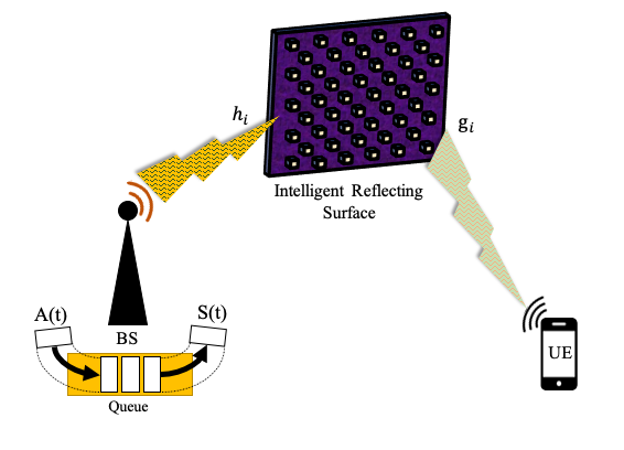
SISO scenario: Let $p_{t}$ be the total transmit power budget of the BS. Let $x$ be the symbol that is transmitted by the BS, then the received signal $y$ at the UE is given as:

where $h_{i}\sim\mathcal{CN}(0,1)$ represents the channel gain from the BS to the $i$-th element of the IRS, and $g_{i}\sim\mathcal{CN}(0,1)$ represents the channel gain from the $i$-th element of the IRS to the UE (see Fig. 1). Moreover, $\phi_{i}\in[0,2\pi)$ is the phase control employed by the controller of the IRS. Furthermore, $\zeta=\frac{G_{t}G_{r}}{(4\pi)^{2}}(\frac{x_{IRS}y_{IRS}}{d_{1}d_{2}})^{2}\cos^{2}(\varphi)$ is the pathloss between the BS and the UE through the IRS [1]. In the preceding pathloss expression, $d_{1}$ represents the distance between the BS and the IRS; $d_{2}$ represents the distance between the IRS and the UE; $\varphi\in[0,\pi/2]$ represents the angle of incidence at the IRS; $x_{IRS}$,$y_{IRS}$ represent the length and the width of the IRS respectively; $G_{t}$, $G_{r}$ represent the antenna gain at the BS and at the UE, respectively. Finally, $w\sim\mathcal{CN}(0,\sigma^{2})$ is the zero-mean, additive white Gaussian noise (AWGN) at the UE with variance $\sigma^{2}$.

Proposition 2.1: The SNR at the UE (during slot $n$) is: $\gamma(n)=\beta\chi_{1}^{2}(\lambda)$, where $\chi_{1}^{2}(\lambda)$ is a non-central chi-square random variable with one degree-of-freedom and non-centrality parameter $\lambda=\frac{N\pi^{2}}{(16-\pi^{2})}>0$. Moreover, $\beta=N\frac{p_{t}\zeta(16-\pi^{2})}{4\sigma^{2}}$.

Proof: Given in Appendix A.

Next, with the SNR $\gamma(n)$ in hand, one can compute the Shannon capacity of the SISO downlink channel under consideration (during slot $n$) as follows:

where $B$ is the bandwidth of the system.

MISO scenario: The BS transmits the same symbol $x$ from all the $N_{t}$ transmit antennas (in order to achieve antenna diversity). Then, the received signal $y$ at the UE is given as:

where $\mathbf{g}^{H}=[g_{1}\ .\ .\ g_{N}]$ , $\mathbf{\Pi}=diag[e^{j\phi_{1}}\ .\ .\ e^{j\phi_{N}}]$ is the so-called reflection coefficients matrix of dimension $N\times N$, $\mathbf{H}$ is the $N\times N_{t}$ channel matrix between the BS and the IRS, and $\mathbf{f}=[f_{1}\ .\ .\ f_{N_{t}}]^{T}$ is the transmit precoding vector at the BS.

Proposition 2.2: The SNR at the UE (during slot $n$) is: $\gamma(n)=p_{t}\zeta\frac{|\mathbf{g}^{H}\mathbf{\Pi}\mathbf{Hf}|^{2}}{\sigma^{2}}$. Specifically, $\gamma(n)$ is an exponential random variable with parameter $\kappa$.

Proof: Given in Appendix B.

Next, with the SNR $\gamma(n)$ in hand, one can compute the Shannon capacity of the MISO downlink channel under consideration (during slot $n$) as: $c(n)=B\ \log_{2}(1+\gamma(n))$.

For a stationary and ergodic channel (service process), the effective capacity (EC) provides the maximum-sustainable constant source rate at the queue of a transmitter, and is given as the limit [13]:

where $\Lambda(\alpha)=\lim_{t\rightarrow\infty}\frac{1}{t}\ln(E(e^{\alpha S(t)}))$ is the Gartner-Ellis limit on the service process given as the LMGF of the cumulative service process $S(t)=\tsum\slimits@_{n=1}^{t}s(n)$ where $s(n)$ is the service process (number of bits successfully served) during time-slot $n$. Moreover, $\alpha>0$ is the so-called QoS exponent. Specifically, when $\alpha$ tends to zero, it implies delay-tolerant communication. On the other hand, when $\alpha$ tends to infinity, it implies delay-limited communication. Note that the EC in Eq. 4 has the units of bits/block.

In short, the notion of the EC allows us to determine the maximum fixed source rate under a statistical QoS constraint—$P(D>D_{m})\leq\epsilon$, where $D$ is the steady-state delay experienced by the packets at the queue of the BS, $D_{m}$ is the delay target, and $\epsilon$ is the delay-violation probability.

When the BS has perfect CSI available, it transmits at the Shannon rate $c(n)$ during slot $n$, which implies that $s(n)=c(n)$. Moreover, due to the assumption A2 which states that the block fading is i.i.d. on both hops (and thus, the service process elements $s(n)$ are i.i.d.), Eq. 4 could be simplified as follows¹¹1The EC is defined as: $EC=\lim_{t\rightarrow\infty}-\frac{1}{\alpha t}\ln(E(e^{-\alpha\tsum\slimits@_{n=1}^{t}s(n)}))$. This expression could be re-written as: $EC=\lim_{t\rightarrow\infty}-\frac{1}{\alpha t}\ln(\Pi_{n}E(e^{-\alpha s(n)}))$. Using the identity $\ln(a.b)=\ln(a)+\ln(b)$, we could re-write EC as follows: $EC=\lim_{t\rightarrow\infty}-\frac{1}{\alpha t}\tsum\slimits@_{n}\ln(E(e^{-\alpha s(n)}))$. Finally, due to the fact that the service process elements $s(n)$ are i.i.d., EC is further simplified as follows: $EC=-\frac{1}{\alpha}\ln(E(e^{-\alpha s(1)}))$, where $s(1)=c(1)$. [22]:

where $s(1)=c(1)$. Next, we compute the moment generating function (MGF) of the service process $s(1)$ during slot 1 as follows:

where $f_{X}(x)$ is the probability density function (pdf) of $X\sim\chi_{1}^{2}(\lambda)$. Next, we do the following relaxation: $(1+\beta x)\approx(\beta x)$. After some simplification, and utilizing a result (Theorem $3.4.1$) from [23], above equation could be re-written as follows:

where $\Gamma(.)$ is the gamma function and $\prescript{}{x}{\mathbf{F}}_{x}(.,.,.)$ is the generalized hypergeometric function. Next, using the fact that $\int_{0}x^{a-1}e^{-bx}\prescript{}{0}{\mathbf{F}}_{1}(;,c,x)dx=b^{-a}\Gamma(a)\prescript{}{1}{\mathbf{F}}_{1}(a,c,\frac{1}{b})$, and after some simplifications, Eq. 7 can be written as:

Finally, putting Eq. III-A into Eq. 5 leads us to the final expression of the EC.

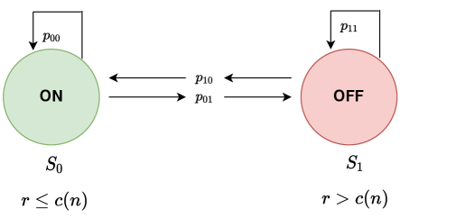
We now compute the EC of the IRS-aided SISO downlink when there is no CSI knowledge available at the BS. In this case, rate adaptation by the BS is not possible; thus, it transmits at a constant rate of $r$ bits/sec during every slot. Then, due to Shannon’s channel capacity limit $c(n)$ (see Eq. 2), the SISO downlink under consideration becomes an ON-OFF channel. Thus, it could be modelled as a Markov chain with two states, namely $S_{0}$ (ON state) and $S_{1}$ (OFF state). That is, when $r\leq c(n)$, then the channel is ON ($rT$ bits are received by the UE), and is in state $S_{0}$. Here, $T$ represents the duration of a time-slot. On the other hand, when $r>c(n)$, then the channel is OFF (zero bits are received by the UE), and is in state $S_{1}$. The motivation behind Markov chain modelling of the SISO downlink comes due to a well-reputed result [24] which states that one viable way to compute the EC is by computing the spectral radius of a special block-companion matrix $\mathbf{P\Theta}$ where $\mathbf{P}$ is the so-called state-transition probability matrix and $\mathbf{\Theta}$ is a diagonal reward matrix. The Markov chain representation of the IRS-aided SISO downlink (for the scenario of no CSI at the BS) is shown in Fig. 2. The entries of the matrix $\mathbf{P}$ for the two-state Markov chain at hand are also labelled in Fig. 2.

The state-transition probability matrix $\mathbf{P}$ of the Markov chain under consideration is formally defined as:

where $p_{xy}$ is the state-transition probability from the state $S_{x}$ during slot $n-1$ to the state $S_{y}$ during slot $n$.

Let’s compute all the four entries of $\mathbf{P}$ one by one. To this end, the probability $p_{00}$ is defined as:

Next, recall the assumption A2 which states that block fading channels are i.i.d. across the slots; thus, the event $r<c(n-1)$ is statistically independent from the event $r<c(n)$. In other words, the stochastic process $\{c(n)\}$ (or, equivalently, the stochastic process $\{\gamma(n)\}$) is a memoryless process. Therefore, if the SISO downlink at hand has evolved to, say, the state $S_{0}$ during slot $n$, then the system is completely oblivious/indifferent of the state ($S_{0}$ or $S_{1}$) it was into during the previous slot $n-1$. This allows us to lead to the conclusion that the elements of the first column of $\mathbf{P}$ are identical: $p_{00}=p_{10}=p_{0}$. Similarly, the elements of the second column of $\mathbf{P}$ are identical: $p_{01}=p_{11}=p_{1}$. Thus, the matrix $\mathbf{P}$ becomes a unit-rank matrix:

Next, we compute $p_{0}$ as follows:

where $Q_{x}(.,.)$ is the Marcum Q-function of order $x$, and $\Xi=\sqrt{\frac{2^{\frac{r}{B}}-1}{\beta}}$. Similarly,

Next, we utilize the findings of [24] to compute the EC as follows:

where $sp(\mathbf{A})$ computes the spectral radius of the matrix $\mathbf{A}$, and $\mathbf{\Theta}$ is a diagonal matrix which contains the MGFs of the service processes for the two states ($S_{0}$ and $S_{1}$) on its main diagonal. In state $S_{0}$, $rT$ bits are received at the UE during a given time-slot; therefore, the MGF of the service process is: $e^{\alpha rT}$. On the other hand, when the system is in state $S_{1}$, zero bits are received at the UE; therefore, the MGF of the service process is: $e^{0}=1$. Thus, the final expression of the EC is as follows:

Computation of the optimal transmission rate. For the scenario of no CSI at the BS, the EC could be maximized further by searching for the optimal transmission rate $r^{*}$ at the BS. This is because we note that Eq. 15 is a concave-like function of $r$. Thus, one could further enhance the EC in Eq. 15 by searching for an optimal transmission rate. This is achieved by taking the derivative of Eq. 15 w.r.t. $r$ and equating it to zero. In other words, $r=\arg\max_{r}EC(r)$. Moreover, Eq. 15 implies that the maximizing the EC is equivalent to minimizing the argument of the $\ln(.)$ on its right-hand side. Therefore,

Taking partial derivative of $\rho(r)=(p_{0}e^{-\alpha rT}+p_{1})$ w.r.t. $r$, we get:

where $Q_{\frac{1}{2}}^{\text{\textdagger}}(\sqrt{\lambda},\Xi)=\frac{\partial Q_{\frac{1}{2}}(\sqrt{\lambda},\Xi)}{\partial\Xi}=-\frac{\Xi^{\frac{1}{2}}}{\lambda^{\frac{-1}{4}}}e^{-\frac{(\lambda+\Xi^{2})}{2}}I_{\frac{-1}{2}}(\sqrt{\lambda}\Xi)$ [25], where $I_{x}(.)$ is the modified Bessel function of order $x$. Now, equating Eq. III-B to zero reveals that solving for $r$ is quite involved due to the presence of infinite number of terms in both the modified Bessel function as well as the Marcum Q-function. Therefore, we propose an alternative approach where we compute $r$ using an iterative, gradient-descent method. Specifically, the gradient-descent method begins with an initial guess $r(0)$ of the transmission rate, and utilizes the following control law to refine its guess of $r$ during iteration $m$:

where $\delta$ is the step size (basically, an algorithm parameter), and $\frac{\partial\rho}{\partial r}$ is the gradient of the EC function (see Eq. III-B) that gets evaluated at $r=r(m-1)$. The algorithm terminates when the following condition is met: $r(m)-r(m-1)\leq\epsilon_{c}$, where $\epsilon_{c}$ is a small constant. If the algorithm terminates, say, during iteration $\mathcal{M}$, it outputs: $r=r(\mathcal{M})$.

Recall that we assume the channel fading/service process elements across the slots on both hops to be i.i.d. Moreover, we assume that the time-window $t$ under consideration is reasonably large so that one could invoke the Central limit theorem to approximate the distribution of the cumulative service process $S(t)=\tsum\slimits@_{n=1}^{t}s(n)$ as Gaussian [19]. Thus, the EC expression in Eq. 4 becomes the LMGF of a Gaussian random variable, and is given as:

where $\mu_{s(1)}$ is the mean of service process $s(1)$, while $\sigma_{s(1)}^{2}$ is the variance of the service process $s(1)$. In other words, to compute the EC, we need to find the first and second moments of the service process. The first moment (mean) is given as:

where $f_{X}(x)=\kappa e^{-\kappa x}$ is the pdf of $X\sim\text{exp}(\kappa)$. Recall that $X$ is the SNR at the UE as defined in Proposition 2.2. In terms of natural-log, the above equation could be expressed as:

Applying integration-by-parts, we have:

where $E_{1}(.)$ is the exponential integral function.

Next, the second moment $\eta_{s(1)}$ of the service process $s(1)$ could be computed as follows:

We follow the steps of [16] to compute the second moment and the final result is given as:

where $C$ is the Euler constant.

Thus, $\sigma_{s(1)}^{2}$ could be computed as follows: $\sigma_{s(1)}^{2}=\eta_{s(1)}-\mu_{s(1)}^{2}$ where $\eta_{s(1)}$, $\mu_{s(1)}$ are given in Eqs. IV-A and IV-A, respectively. Finally, plugging the values of $\sigma_{s(1)}^{2}$ and $\mu_{s(1)}$ into Eq. 19 lead us to final expression of the EC.

We now compute the EC of the IRS-aided MISO system when there is no CSI knowledge at the BS. As we will see, the conceptual framework is the same as the IRS-aided SISO system with no CSI at the BS. That is, the BS transmits at a fixed rate $r$. Consequently, the MISO downlink channel under consideration becomes an ON-OFF channel. In other words, the system could be modelled as a Markov chain with two states, whereby the state $S_{0}$ represents the ON state, while the state $S_{1}$ represents the OFF state (see Fig. 2).

Having modelled the MISO downlink as a Markov chain, we need to find the state transition probabilities as well as the MGFs of service processes during the two states $S_{0}$ and $S_{1}$. The matrix $\mathbf{P}$ turns out to be a rank-1 matrix again; and thus, its two entries are given below:

The MGFs remain the same as before. Finally, the EC is given as:

Computation of the optimal transmission rate. Once again, for the scenario of no CSI at the BS, the EC of the IRS-aided MISO system could be maximized further by searching for the optimal rate $r^{*}$ at the BS. This is done by taking the derivative of Eq. 25 w.r.t. $r$ and equating it to zero. Doing so, and after simplification we get the following transcendental equation:

One potential way to solve above equation is to assume $e^{\alpha rT}-1\approx e^{\alpha rT}$ which in turn implies that $e^{\alpha rT}>>1$. Under this assumption, the optimal transmission rate is given as:

Fig. 3 plots the EC of the SISO downlink against the total power budget $p_{t}$ of the BS when it has the perfect CSI at its disposal. Fig. 3 reveals the following: i) there is a logarithmic increase in the EC with the increase in $p_{t}$ (because ultimately, the EC is a variant of the Shannon’s capacity, and is defined as the log of the MGF of the service process); ii) there is also a logarithmic increase in the EC with the increase in the number of IRS elements $N$ (but note that increasing $N$ also increases IRS hardware cost as well as the CSI acquisition overhead at the BS and at the IRS); iii) the EC of the delay-tolerant communication (figure on the left with $\alpha=0.1$) is significantly (more than ten-fold) larger than the EC of the delay-limited communication (figure on the right with $\alpha=10$).

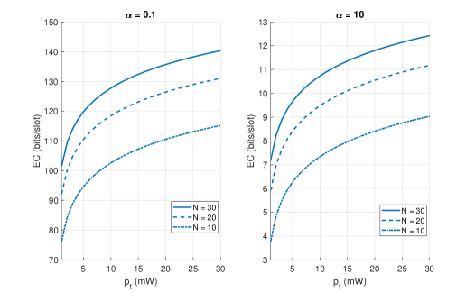
Fig. 4 is the repeat of Fig. 3 for the case when the CSI is not available at the BS. Not only that, the key points learned from the Fig. 4 are also the same as the Fig. 3. Furthermore, a quick comparison of the two figures (Fig. 3 and Fig. 4) reveals that the presence of the CSI at the BS has a significant positive impact on the EC (for both delay-tolerant and delay-limited communication regimes). Specifically, the EC for the case of perfectly-known CSI at the BS is at least five times greater than the EC for the case of no CSI at the BS. Note that the optimal transmission rate $r$ was computed and thereafter utilized to compute the EC for Fig. 4.

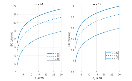
Fig. 5 plots the EC of the MISO downlink against the total power budget $p_{t}$ of the BS when it has the perfect CSI at its disposal. Fig. 5 lets us infer similar trends as in Fig. 3. That is, the EC increases logarithmically with the increase in $p_{t}$ as well as with the increase in the number of IRS elements $N$. Moreover, the EC of the delay-tolerant communication (figure on the left with $\alpha=0.1$) is significantly (at least three times) larger than the EC of the delay-limited communication (figure on the right with $\alpha=10$). Last but not the least, a quick comparison of Fig. 5 with Fig. 3 reveals a gain of at least 30 bits/slot in the EC due to the presence of multiple antennas ($N_{t}=10$, in this case) at the BS, for medium-to-high values of $p_{t}$.

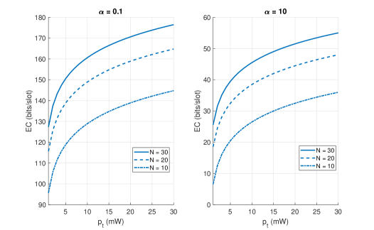
Fig. 6 is again the repeat of Fig. 5 for the case when the CSI is not available at the BS. Not only that, the key points learned from the Fig. 6 are also the same as the Fig. 5. Furthermore, a quick comparison of the two figures (Fig. 5 and Fig. 6) reveals that the lack of the CSI at the BS has an adverse effect on the EC (for both delay-tolerant and delay-limited communication regimes). Specifically, the EC reported in Fig. 6 is at least five times lower than the EC reported in Fig. 5. Last but not the least, comparing Fig. 6 with Fig. 4, we observe a gain of at least 5 bits/slot in the EC of the MISO downlink compared to the EC of the SISO downlink (for the delay-tolerant communication regime). On the other hand, for the delay-limited communication regime, the gain in the EC of the MISO downlink over the EC of the SISO downlink is negligible, due to very strict QoS constraints. Note once gain that the optimal transmission rate $r$ was computed and thereafter utilized to compute the EC for Fig. 6.

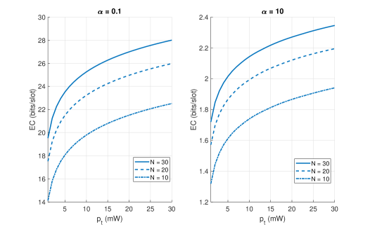
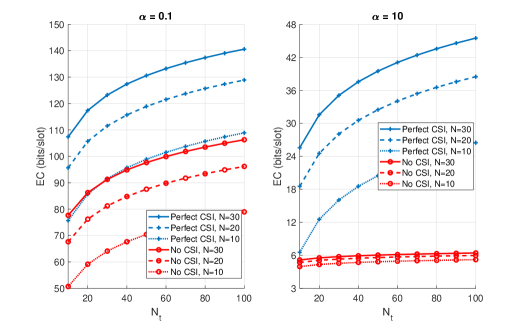
Fig. 7 plots the EC against the number of transmit antennas $N_{t}$ at the BS, for the delay-tolerant communication regime with $\alpha=0.1$ (sub-plot on the left) and the delay-limited communication regime with $\alpha=10$ (sub-plot on the right). Moreover, each of the two sub-plots considers the two extreme cases of the availability of the CSI at the BS (i.e., perfect CSI and no CSI) for various values of the number of IRS elements $N$. We first discuss the delay-tolerant communication regime (sub-plot on the left). Here, we observe that the EC for the case of perfect CSI at the BS is at least 30 bits/slot more than the EC for the case of no CSI at the BS, for a given $N$ and and for any value of $N_{t}$. Moreover, we observe a logarithmic increase in the EC with the increase in an increase in either $N_{t}$ or $N$. Next, the delay-limited communication regime (sub-plot on the right). Here, the most important finding is that we don’t observe any gains in the EC with increase in $N_{t}$ for the pessimistic case of delay-limited communication with no CSI, as expected. This is because the lack of CSI and very strict QoS requirements ($\alpha=10$) together act like a dual-edge sword which eventually diminish any potential gains in the EC due to increase in either $N_{t}$ or $N$.

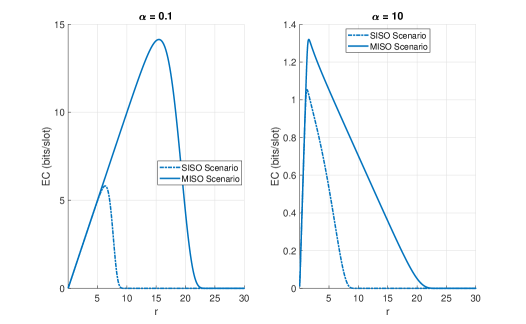
Finally, Fig. 8 plots the EC against the transmission rate $r$ for the delay-tolerant communication regime with $\alpha=0.1$ (see the sub-plot on the left) and the delay-limited communication regime with $\alpha=10$ (see the sub-plot on the right), for the case of no CSI at the BS. Moreover, each of the two sub-plots considers both SISO and MISO scenarios. Fig. 8 corroborates our conjecture that the EC is a concave-like function of $r$. This revelation allows us to find the optimal transmission rate $r$ to enhance the EC further for the case of no CSI at the BS. Note that we kept $p_{t}=1$ mW, and $N_{t}=10$ (for MISO scenario) to generate Fig. 8.

References

- [1] O. Ozdogan, E. Bjornson, and E. G. Larsson, “Intelligent reflecting surfaces: Physics, propagation, and pathloss modeling,” IEEE Wireless Communications Letters, pp. 581–585, May 2019.
- [2] S. Gong, X. Lu, D. T. Hoang, D. Niyato, L. Shu, D. I. Kim, and Y.-C. Liang, “Toward smart wireless communications via intelligent reflecting surfaces: A contemporary survey,” IEEE Communications Surveys & Tutorials, vol. 22, no. 4, pp. 2283–2314, 2020.
- [3] J. Zhao, “A survey of intelligent reflecting surfaces (irss): Towards 6g wireless communication networks,” arXiv e-prints, Nov. 2019.
- [4] C. Huang, S. Hu, G. C. Alexandropoulos, A. Zappone, C. Yuen, R. Zhang, M. D. Renzo, and M. Debbah, “Holographic mimo surfaces for 6g wireless networks: Opportunities, challenges, and trends,” IEEE Wireless Communications, vol. 27, no. 5, pp. 118–125, Oct. 2020.
- [5] Q. Wu and R. Zhang, “Towards smart and reconfigurable environment: Intelligent reflecting surface aided wireless network,” IEEE Communications Magazine, vol. 58, no. 1, pp. 106–112, Jan. 2020.
- [6] C. Huang, A. Zappone, G. C. Alexandropoulos, M. Debbah, and C. Yuen, “Reconfigurable intelligent surfaces for energy efficiency in wireless communication,” IEEE Transactions on Wireless Communications, vol. 18, no. 8, pp. 4157–4170, Aug. 2019.
- [7] X. Yu, D. Xu, and R. Schober, “Enabling Secure Wireless Communications via Intelligent Reflecting Surfaces,” arXiv e-prints, p. arXiv:1904.09573, Apr. 2019.
- [8] Q. Wu and R. Zhang, “Intelligent reflecting surface enhanced wireless network: Joint active and passive beamforming design,” in IEEE Global Communications Conference (GLOBECOM), Dec. 2018, pp. 1–6.
- [9] M.-M. Zhao, Q. Wu, M.-J. Zhao, and R. Zhang, “Intelligent reflecting surface enhanced wireless network: Two-timescale beamforming optimization,” arXiv e-prints, Sep. 2020.
- [10] G. Zhou, C. Pan, H. Ren, K. Wang, and A. Nallanathan, “A framework of robust transmission design for irs-aided miso communications with imperfect cascaded channels,” IEEE Transactions on Signal Processing, vol. 68, pp. 5092–5106, Aug. 2020.
- [11] M.-M. Zhao, Q. Wu, M.-J. Zhao, and R. Zhang, “Exploiting amplitude control in intelligent reflecting surface aided wireless communication with imperfect csi,” arXiv e-prints, May 2020.
- [12] C. Huang, R. Mo, and C. Yuen, “Reconfigurable intelligent surface assisted multiuser miso systems exploiting deep reinforcement learning,” IEEE Journal on Selected Areas in Communications, vol. 38, no. 8, pp. 1839–1850, jun. 2020.
- [13] D. Wu and R. Negi, “Effective capacity: a wireless link model for support of quality of service,” IEEE Trans. Wireless Commun., vol. 2, no. 4, pp. 630–643, Jul. 2003.
- [14] S. Akin and M. C. Gursoy, “Effective capacity analysis of cognitive radio channels for quality of service provisioning,” IEEE Trans. Wireless Commun., vol. 9, no. 11, pp. 3354–3364, Nov. 2010.
- [15] A. H. Anwar, K. G. Seddik, T. ElBatt, and A. H. Zahran, “Effective capacity of delay-constrained cognitive radio links exploiting primary feedback,” IEEE Trans. Veh. Tech., vol. 65, no. 9, pp. 7334–7348, Sep. 2016.
- [16] J. Gross, “Scheduling with outdated csi: Effective service capacities of optimistic vs. pessimistic policies,” in Proc. Workshop on Quality of Service, 2012, pp. 1–9.
- [17] D. Qiao, M. C. Gursoy, and S. Velipasalar, “Effective capacity of two-hop wireless communication systems,” IEEE Trans. Info. Theory, vol. 59, no. 2, pp. 873–885, Feb. 2013.
- [18] S. Ren and K. B. Letaief, “Maximizing the effective capacity for wireless cooperative relay networks with qos guarantees,” IEEE Trans. Commun., vol. 57, no. 7, pp. 2148–2159, Jul. 2009.
- [19] B. Soret, M. C. Aguayo-Torres, and J. T. Entrambasaguas, “Capacity with explicit delay guarantees for generic sources over correlated rayleigh channel,” IEEE Trans. Wireless Commun., vol. 9, no. 6, pp. 1901–1911, Jun. 2010.
- [20] S. W. H. Shah, M. M. U. Rahman, A. N. Mian, A. Imran, S. Mumtaz, and O. A. Dobre, “On the impact of mode selection on effective capacity of device-to-device communication,” IEEE Wireless Commun. Lett., vol. 8, no. 3, pp. 945–948, Jun. 2019.
- [21] W. Aman, Z. Haider, S. W. H. Shah, M. M. Ur Rahman, and O. A. Dobre, “On the effective capacity of an underwater acoustic channel under impersonation attack,” in IEEE International Conference on Communications (ICC), Jul. 2020.
- [22] J. Tang and X. Zhang, “Quality-of-service driven power and rate adaptation over wireless links,” IEEE Transactions on Wireless Communications, vol. 6, no. 8, pp. 3058–3068, Dec. 2007.
- [23] R. Muirhead, Aspects of multivariate statistical theory, ser. Wiley Series in Probability and Mathematical Statistics. John Wiley & Sons New York, 1982.
- [24] C. Chang, Performance Guarantees in Communication Networks, ser. Telecommun. Netw. and Computer Syst. Springer London, 2012.
- [25] Y. A. Brychkov, “On some properties of the marcum q function,” Integral Transforms and Special Functions, vol. 23, no. 3, pp. 177–182, 2012.