On the fitting of mixtures of multivariate skew $t$ -distributions via the EM algorithm

Sharon Lee, Geoffrey J. McLachlan
Department of mathematics, the University of Queensland,
Brisbane, Australia

Abstract

We show how the expectation-maximization (EM) algorithm can be applied exactly for the fitting of mixtures of a general multivariate skew $t$ (MST) distributions, eliminating the need for computationally expensive Monte Carlo estimation. Finite mixtures of MST distributions have proven to be useful in modelling heterogeneous data with asymmetric and heavy tail behaviour. Recently, they have been exploited as an effective tool for modelling flow cytometric data. However, without restrictions on the the characterizations of the component skew $t$ -distributions, Monte Carlo methods have been used to fit these models. In this paper, we show how the EM algorithm can be implemented for the iterative computation of the maximum likelihood estimates of the model parameters without resorting to Monte Carlo methods for mixtures with unrestricted MST components. The fast calculation of semi-infinite integrals on the E-step of the EM algorithm is effected by noting that they can be put in the form of moments of the truncated multivariate $t$ -distribution, which subsequently can be expressed in terms of the non-truncated form of the $t$ -distribution function for which fast algorithms are available. We demonstrate the usefulness of the proposed methodology by some applications to three real data sets.

1 Introduction

Finite mixture distributions have become increasingly popular in the modelling and analysis of data due to their flexibility. This use of finite mixture distributions to model heterogeneous data has undergone intensive development in the past decades, as witnessed by the numerous applications in various scientific fields such as bioinformatics, cluster analysis, genetics, information processing, medicine, and pattern recognition. Comprehensive surveys on mixture models and their applications can be found, for example, in the monographs by Everitt and Hand (1981), Titterington, Smith, and Markov (1985), Lindsay (1995), McLachlan and Basford (1988), and McLachlan and Peel (2000), among others; see also the papers by Banfield and Raftery (1993) and Fraley and Raftery (1999).

Mixtures of multivariate $t$ -distributions, as proposed by McLachlan and Peel (1998, 2000), provide extra flexibility over normal mixtures. The thickness of tails can be regulated by an additional parameter – the degrees of freedom, thus enabling it to accommodate outliers better than normal distributions. However, in many practical problems, the data often involve observations whose distributions are highly asymmetric as well as having longer tails than the normal, for example, datasets from flow cytometry (Pyne et al., 2009). Azzalini (1985) introduced the so-called skew-normal (SN) distribution for modelling symmetry in data sets. Following the development of the SN and skew $t$ -mixture models by Lin, Lee, and Yen (2007), and Lin, Lee, and Hsieh (2007), respectively, Basso et al. (2010) studied a class of mixture models where the components densities are scale mixtures of skew-normal distributions introduced by Branco and Dey (2001), which include the classical skew-normal and skew $t$ -distributions as special cases. Recently, Cabral, Lachos, and Prates (2012) have extended the work of Basso et al. (2010) to the multivariate case.

In a study of automated flow cytometry analysis, Pyne et al. (2009) proposed a finite mixture of multivariate skew $t$ -distributions based on a ‘restricted’ variant of the skew $t$ -distribution introduced by Sahu, Dey, and Branco (2003). Lin (2010) considered a similar approach, but working with the original (unrestricted) characterization by Sahu et al. (2003). However, with this more general formulation, maximum likelihood (ML) estimation via the EM algorithm (Dempster, Laird, and Rubin, 1977) can no longer be implemented in closed form due to the intractability of some of the conditional expectations involved on the E-step. To work around this, Lin (2010) proposed a Monte Carlo (MC) version of the E-step. One potential drawback of this approach is that the model fitting procedure relies on MC estimates which can be computationally expensive.

In this paper, we show how the EM algorithm can be implemented exactly to calculate the ML estimates of the parameters for the (unrestricted) multivariate skew $t$ -mixture model, based on analytically reduced expressions for the conditional expectations, suitable for numerical evaluation using readily available software. A key factor in being able to compute the integrals quickly by numerical means is the recognition that they can be expressed as moments of a truncated multivariate $t$ -distribution, which in turn can be expressed in terms of the distribution function of a (non-truncated) multivariate central $t$ -random vector, for which fast programs already exist. We show that the proposed algorithm is highly efficient compared to the version with a MC E-step. It produces highly accurate results for which, if MC were to achieve comparable accuracy, a large number of draws would be necessary.

The remainder of the paper is organized as follows. In Section 2, for the sake of completeness, we include a brief description of the multivariate skew $t$ -distribution (MST) used for defining the multivariate skew $t$ -mixture model. We also describe the truncated $t$ -distribution in the multivariate case, critical for the swift evaluation of the integrals on the E-step occurring in the calculation of some of the conditional expectations. Section 3 presents the development of an EM algorithm for obtaining ML estimates for the MST distribution. In the following section, the finite mixture of MST (FM-MST) distributions is defined. Section 5 presents an implementation of the EM algorithm to the fitting of the FM-MST model. An approximation to the observed information matrix is discussed in Section 6. Finally, we present some applications of the proposed methodology in Section 7.

2 Preliminaries

We begin by defining the multivariate skew $t$ -distribution and briefly describing some related properties. Some alternative versions of the distribution are also discussed. Next, we introduce the truncated multivariate $t$ -distribution and provide some formulas for computing its moments. These expressions are crucial for the swift evaluation of the conditional expectations on the E-step to be discussed in the next section.

2.1 The Multivariate Skew $t$ -Distribution

Following Sahu et al. (2003), a random vector $\boldsymbol{Y}$ is said to follow a $p$ -dimensional (unrestricted) skew $t$ -distribution with $p\times 1$ location vector $\boldsymbol{\mu}$ , $p\times p$ scale matrix $\boldsymbol{\Sigma}$ , $p\times 1$ skewness vector $\boldsymbol{\delta}$ , and scalar degrees of freedom $\nu$ , if its density is given by

f_{p}(\boldsymbol{y};\boldsymbol{\mu},\boldsymbol{\Sigma},\boldsymbol{\delta},\nu)=2^{p}t_{p,\nu}\left(\boldsymbol{y};\boldsymbol{\mu},\boldsymbol{\Omega}\right)T_{p,\nu+p}\left(\boldsymbol{y}^{*};\boldsymbol{0},\boldsymbol{\Lambda}\right),

(1)

where

	$\displaystyle\boldsymbol{\Delta}$	$\displaystyle=\mbox{diag}(\boldsymbol{\delta}),$
	$\displaystyle\boldsymbol{\Omega}$	$\displaystyle=\boldsymbol{\Sigma}+\boldsymbol{\Delta}\boldsymbol{\Delta}^{T},$
	$\displaystyle\boldsymbol{y}^{*}$	$\displaystyle=\boldsymbol{q}\sqrt{\frac{\nu+p}{\nu+d\left(\boldsymbol{y}\right)}},$
	$\displaystyle\boldsymbol{q}$	$\displaystyle=\boldsymbol{\Delta}^{T}\boldsymbol{\Omega}^{-1}(\boldsymbol{y}-\boldsymbol{\mu}),$
	$\displaystyle d\left(\boldsymbol{y}\right)$	$\displaystyle=(\boldsymbol{y}-\boldsymbol{\mu})^{T}\boldsymbol{\Omega}^{-1}(\boldsymbol{y}-\boldsymbol{\mu}),$
	$\displaystyle\boldsymbol{\Lambda}$	$\displaystyle=\boldsymbol{I}_{p}-\boldsymbol{\Delta}^{T}\boldsymbol{\Omega}^{-1}\boldsymbol{\Delta}.$

Here the operator $\mbox{diag}(\boldsymbol{\delta})$ denotes a diagonal matrix with diagonal elements specifed by the vector $\boldsymbol{\delta}$ . Also, we let $t_{p,\nu}(.;\boldsymbol{\mu},\boldsymbol{\Sigma})$ be the $p$ -dimensional $t$ -density with location vector $\boldsymbol{\mu}$ , scale matrix $\boldsymbol{\Sigma}$ , and degrees of freedom $\nu$ , and $T_{p,\nu}(.;\boldsymbol{\mu},\boldsymbol{\Sigma})$ the corresponding (cumulative) distribution function. The notation $\boldsymbol{Y}\sim\mbox{ST}_{p,\nu}(\boldsymbol{\mu},\boldsymbol{\Sigma},\boldsymbol{\delta})$ will be used. Note that when $\boldsymbol{\delta}=\boldsymbol{0}$ , (1) reduces to the symmetric $t$ -density $t_{p,\nu}(\boldsymbol{y};\boldsymbol{\mu},\boldsymbol{\Sigma})$ . Also, when $\nu\rightarrow\infty$ , we obtain the skew normal distribution.

The MST distribution admits a convenient hierarchical form,

$\displaystyle\boldsymbol{Y}\mid\boldsymbol{u},w$	$\displaystyle\sim$	$\displaystyle N_{p}\left(\boldsymbol{\mu}+{\boldsymbol{\Delta}}\boldsymbol{u},\textstyle\frac{1}{w}{\boldsymbol{\Sigma}}\right),$
$\displaystyle\boldsymbol{U}\mid w$	$\displaystyle\sim$	$\displaystyle HN_{p}\left(\boldsymbol{0},\frac{1}{w}\boldsymbol{I}_{p}\right),$
$\displaystyle W$	$\displaystyle\sim$	$\displaystyle\mbox{gamma}\left(\frac{\nu}{2},\frac{\nu}{2}\right),$

where $\boldsymbol{I}_{p}$ is the $p\times p$ identity matrix, $N_{k}(\boldsymbol{\mu},\boldsymbol{\Sigma})$ denotes the multivariate normal distribution with mean $\boldsymbol{\mu}$ and covariance matrix $\boldsymbol{\Sigma}$ , $HN_{p}(\boldsymbol{0},\boldsymbol{\Sigma})$ represents the $p$ -dimensional half-normal distribution with mean $\boldsymbol{0}$ and scale matrix $\boldsymbol{\Sigma}$ , and $\mbox{gamma}(\alpha,\beta)$ is the Gamma distribution with mean $\alpha/\beta$ .

We observe from (LABEL:MST_H) that the MST distribution (1) has the following stochastic representation. Suppose that conditional on the value $w$ of the gamma random variable $W$ ,

\left(\begin{array}[]{c}\boldsymbol{U}_{0}\\ \boldsymbol{U}\end{array}\right)\sim N_{p}\left(\left(\begin{array}[]{c}\boldsymbol{\mu}\\ \boldsymbol{0}\end{array}\right),\left(\begin{array}[]{cc}\boldsymbol{\Sigma}/w&\boldsymbol{0}\\ \boldsymbol{0}&\boldsymbol{I}_{p}/w\end{array}\right)\right),

(3)

where $\boldsymbol{I}_{p}$ denotes the $p\times p$ identity matrix, $\boldsymbol{0}$ denotes the zero vector of appropriate dimension, and $\boldsymbol{U}_{0}$ is a $p$ -dimensional random vector. Then

\boldsymbol{Y}=\boldsymbol{\Delta}\left|\boldsymbol{U}\right|+\boldsymbol{U}_{0}

(4)

has the multivariate skew $t$ -distribution density (1). In the above, $\left|\boldsymbol{U}\right|$ denotes the vector whose $i$ th element is the magnitude of the $i$ th element of the vector $\boldsymbol{U}$ . It is important to note that, although also known as the multivariate skew $t$ -distribution, the versions considered by Azzalini and Dalla Valle (1996), Gupta (2003), and Lachos, Ghosh, and Arellano-Valle (2010), among others, are different from (1). These versions are simpler in that the skew $t$ -density is defined in terms involving only the univariate $t$ -distribution function instead of the multivariate form of the latter as used in (1). Recently, Pyne et al. (2009) proposed a simplified version of the skew $t$ -density given by (1) by replacing the term $\boldsymbol{\Delta}\left|\boldsymbol{U}\right|$ in (4) by the term $\boldsymbol{\delta}\left|U\right|$ , where $U$ is a univariate central $t$ -random variable with $\nu$ degrees of freedom, leading to the reduced skew $t$ -density:

2^{p}t_{p,\nu}\left(\mbox{\boldmath$y$};\boldsymbol{\mu},\boldsymbol{\Sigma}\right)T_{1,\nu+p}\left(y_{1}^{*};0,1\right),

(5)

where $y_{1}^{*}=\left[\left(\nu+p\right)/\left(\nu+d\left(\mbox{\boldmath$y$}\right)\right)\right]^{\frac{1}{2}}\boldsymbol{\delta}^{T}\boldsymbol{\Omega}^{-1}(\mbox{\boldmath$y$}-\boldsymbol{\mu})$ . We shall refer to this characterization of skew $t$ -distribution as the ‘restricted’ multivariate skew $t$ (rMST)distribution. One immediate consequence of this type of ‘simplification’ is that the correlation structure of the original symmetric model is affected by the introduction of skewness, whereas for (1) the correlation structure remains the same, as noted in Arellano-Valle, Bolfarine, and Lachos (2007). Nevertheless, one major advantage of having simplified forms like (5) is that calculations on the E-step can be expressed in closed form. However, the form of skewness is limited in these characterizations. Here, we extend their approach to the more general form of the skew $t$ -density as proposed by Sahu et al. (2003).

2.2 The truncated multivariate $t$ -distribution

Let $\boldsymbol{X}$ be a $p$ -dimensional random variable having a multivariate $t$ -distribution with location vector $\boldsymbol{\mu}$ , scale matrix $\boldsymbol{\Sigma}$ , and $\nu$ degrees of freedom. Truncating $\boldsymbol{x}$ to the hyperplane region $\mathbb{A}=\left\{\boldsymbol{x}\leq\boldsymbol{a},\;\boldsymbol{a}\in\mathbb{R}^{p}\right\}$ , where $\boldsymbol{x}\leq\boldsymbol{a}$ means each element $x_{i}=(\boldsymbol{x})_{i}$ is less than or equal to $a_{i}=(\boldsymbol{a})_{i}$ for $i=1,\ldots,p$ , results in a right-truncated $t$ -distribution whose density is given by

f_{\mathbb{A}}(\boldsymbol{x};\boldsymbol{\mu},\boldsymbol{\Sigma},\nu)=T_{p,\nu}^{-1}\left(\boldsymbol{a};\boldsymbol{\mu},\boldsymbol{\Sigma}\right)t_{p,\nu}\left(\boldsymbol{x};\boldsymbol{\mu},\boldsymbol{\Sigma},\nu\right),\;\;\;\;\boldsymbol{x}\in\mathbb{A}.

(6)

For a random vector $\boldsymbol{X}$ with density (6), we write $\boldsymbol{X}\sim tt_{p,\nu}\left(\boldsymbol{\mu},\boldsymbol{\Sigma};\mathbb{A}\right)$ . For our purposes, we will be concerned with the first two moments of $\boldsymbol{X}$ , specifically $E(\boldsymbol{X})$ and $E(\boldsymbol{X}\boldsymbol{X}^{T})$ . Explicit formulas for the truncated central $t$ -distribution in the univariate case $tt_{1,\nu}\left(0,\sigma^{2};\mathbb{A}\right)$ were provided by O’Hagan (1973), who expressed the moments in terms of the non-truncated $t$ -distribution. The multivariate case was studied in O’Hagan (1976), but still considering the central case only. We will generalize these results to the case with non-zero location vector here.

Before presenting the expressions, it will be convenient to introduce some notation. Let $\boldsymbol{x}$ be a vector, where $x_{i}$ denotes the $i$ th element and $\boldsymbol{x}_{ij}$ is a two-dimensional vector with elements $x_{i}$ and $x_{j}$ . Also, $\boldsymbol{x}_{-i}$ and $\boldsymbol{x}_{-ij}$ represents the $(p-1)$ and $(p-2)$ -dimensional vector, respectively, with the corresponding elements removed. For a matrix $\boldsymbol{X}$ , $x_{ij}$ denotes the $ij$ th element, and $\boldsymbol{X}_{ij}$ defines the $2\times 2$ matrix consisting of the elements $x_{ii}$ , $x_{ij}$ , $x_{ji}$ and $x_{jj}$ . $\boldsymbol{X}_{-i}$ is created by removing the $i$ th row and column from $\boldsymbol{X}$ . Similarly, $\boldsymbol{X}_{-ij}$ is the $(p-2)$ -dimensional square matrix resulting from the removal of the $i$ th and $j$ th row and column from $\boldsymbol{X}$ . Lastly, $\boldsymbol{X}_{(ij)}$ is the $i$ th and $j$ th column of $\boldsymbol{X}$ with the elements of $\boldsymbol{X}_{ij}$ removed, yielding a $(p-2)\times 2$ matrix. We now proceed to the expressions for the first two moments of $\boldsymbol{X}$ .

With some effort, one can show that the first moment of (6) is

\displaystyle E\left(\boldsymbol{X}\right)

\displaystyle=\boldsymbol{\mu}-c^{-1}\boldsymbol{\Sigma}\boldsymbol{\xi}=\boldsymbol{\mu}-\boldsymbol{\mu}^{*},

(7)

where $c=T_{p,\nu}\left(\boldsymbol{a}-\boldsymbol{\mu};\boldsymbol{0},\boldsymbol{\Sigma}\right)$ , and $\boldsymbol{\xi}$ is a $p\times 1$ vector with elements

\displaystyle\xi_{i}

\displaystyle=\left(2\pi\sigma_{ii}\right)^{-\frac{1}{2}}\left(\frac{\nu}{\nu+\sigma_{ii}^{-1}(a_{i}-\mu_{i})^{2}}\right)^{(\frac{\nu-1}{2})}\frac{\Gamma\left(\frac{\nu-1}{2}\right)}{\Gamma\left(\frac{\nu}{2}\right)}\sqrt{\frac{\nu}{2}}T_{p-1,\nu-1}\left(a^{*};\boldsymbol{0},\boldsymbol{\Sigma}^{*}\right),

for $i=1,\ldots,p$ , and where

	$\displaystyle\boldsymbol{a}^{*}$	$\displaystyle=\left(\boldsymbol{a}_{-i}-\boldsymbol{\mu}_{-i}\right)-\left(\boldsymbol{a}_{i}-\boldsymbol{\mu}_{i}\right)\sigma_{ii}^{-1}\boldsymbol{\Sigma}_{(i)}$
and
	$\displaystyle\boldsymbol{\Sigma}^{*}$	$\displaystyle=\left(\frac{\nu+\sigma_{ii}^{-1}\left(a_{i}-\mu_{i}\right)^{2}}{\nu-1}\right)\left(\boldsymbol{\Sigma}_{-i}-\frac{1}{\sigma_{ii}}\boldsymbol{\Sigma}_{(i)}\boldsymbol{\Sigma}_{(i)}^{T}\right).$

The second moment is given by

	$\displaystyle E\left(\boldsymbol{X}\boldsymbol{X}^{T}\right)$	$\displaystyle=$	$\displaystyle\boldsymbol{\mu}\boldsymbol{\mu}^{T}-\boldsymbol{\mu}\boldsymbol{\mu}^{^{T}}-\boldsymbol{\mu}^{}\boldsymbol{\mu}^{T}-c^{-1}\boldsymbol{\Sigma}\boldsymbol{H}\boldsymbol{\Sigma}$		(8)
			$\displaystyle+c^{-1}\left(\textstyle\frac{\nu}{\nu-2}\right)T_{p,\nu-2}\left(\boldsymbol{a}-\boldsymbol{\mu};\boldsymbol{0},\left(\textstyle\frac{\nu}{\nu-2}\right)\boldsymbol{\Sigma}\right)\boldsymbol{\Sigma},$		(8)

where $\boldsymbol{H}$ is a $p\times p$ matrix with off-diagonal elements

h_{ij}=-\frac{1}{2\pi\sqrt{\sigma_{ii}\sigma_{jj}-\sigma_{ij}^{2}}}\left(\frac{\nu}{\nu-2}\right)\left(\frac{\nu}{\nu^{*}}\right)^{\frac{\nu}{2}-1}T_{p-2,\nu-2}\left(\boldsymbol{a}^{**};\boldsymbol{0},\boldsymbol{\Sigma}^{**}\right),\;\;i\neq j,

and diagonal elements,

	$\displaystyle h_{ii}$	$\displaystyle=\sigma_{ii}^{-1}(a_{i}-\mu_{i})\xi_{i}-\sigma_{ii}^{-1}\sum_{j\neq i}\sigma_{ij}h_{ij},$
and
	$\displaystyle\nu^{*}$	$\displaystyle=\nu+\left(\boldsymbol{a}_{ij}-\boldsymbol{\mu}_{ij}\right)^{T}\boldsymbol{\Sigma}_{ij}^{-1}\left(\boldsymbol{a}_{ij}-\boldsymbol{\mu}_{ij}\right),$
	$\displaystyle\boldsymbol{a}^{**}$	$\displaystyle=\left(\boldsymbol{a}_{-ij}-\boldsymbol{\mu}_{-ij}\right)-\boldsymbol{\Sigma}_{(ij)}\boldsymbol{\Sigma}_{ij}^{-1}\left(\boldsymbol{a}_{ij}-\boldsymbol{\mu}_{ij}\right),$
	$\displaystyle\boldsymbol{\Sigma}^{**}$	$\displaystyle=\frac{\nu^{*}}{\nu-2}\left(\boldsymbol{\Sigma}_{-ij}-\boldsymbol{\Sigma}_{(ij)}\boldsymbol{\Sigma}_{ij}^{-1}\boldsymbol{\Sigma}_{(ij)}^{T}\right).$

It is worth noting that evaluation of the expressions (7) and (8) rely on algorithms for computing the multivariate central $t$ -distribution function for which highly efficient procedures are readily available in many statistical packages. For example, an implementation of Genz’s algorithm (Genz and Bretz, 2002; Kotz and Nadarajah, 2004) is provided by the mvtnorm package available from the R website.

3 ML Estimation for the MST Distribution

In this section, we describe an EM algorithm for the ML estimation of the MST distribution specified by (1). To apply the EM algorithm, the observed data vector $\boldsymbol{y}=\left(\boldsymbol{y}_{1}^{T},\ldots,\boldsymbol{y}_{n}^{T}\right)^{T}$ is regarded as incomplete, and we introduce two latent variables denoted by $\boldsymbol{u}$ and $w$ , as defined by (LABEL:MST_H). We let $\boldsymbol{\theta}$ be the parameter containing the elements of the location parameter $\boldsymbol{\mu}$ , the distinct elements of the scale matrix $\boldsymbol{\Sigma}$ , the elements of the skew parameter $\boldsymbol{\delta}$ , and the degrees of freedom $\nu$ . It follows that the complete-data log-likelihood function for $\boldsymbol{\theta}$ is given by

$\displaystyle\log L_{c}(\boldsymbol{\theta};\boldsymbol{y},\boldsymbol{u},w)$	$\displaystyle=$	$\displaystyle K-\textstyle\frac{1}{2}n\log\left\|\boldsymbol{\Sigma}\right\|-n\log\Gamma\left(\textstyle\frac{1}{2}\nu\right)+\textstyle\frac{1}{2}n\nu\log\left(\textstyle\frac{1}{2}\nu\right)$	(9)
		$\displaystyle-\textstyle\frac{1}{2}w\left(d\left(\boldsymbol{y}\right)+\left(\boldsymbol{u}-\boldsymbol{q}\right)^{T}\boldsymbol{\Lambda}^{-1}\left(\boldsymbol{u}-\boldsymbol{q}\right)\right)$
		$\displaystyle+\left(\textstyle\frac{1}{2}\nu+p-1\right)\log(w),$

where $K$ does not depend on $\boldsymbol{\theta}$ .

The implementation of the EM algorithm requires alternating repeatedly the E- and M-steps until convergence in the case where the sequence of the log likelihood values ${L(\boldsymbol{\theta}^{(k)})}$ is bounded above. Here $\boldsymbol{\theta}^{(k)}$ denotes the value of $\boldsymbol{\theta}$ after the $k$ th iteration.

On the $(k+1)$ th iteration, the E-step requires the calculation of the conditional expectation of the complete-data log likelihood given the observed data $\boldsymbol{y}$ , using the current estimate $\boldsymbol{\theta}^{(k)}$ for $\boldsymbol{\theta}$ . That is, we have to calculate the so-called $Q$ -function defined by

Q(\boldsymbol{\theta};\boldsymbol{\theta}^{(k)})=E_{\boldsymbol{\theta}^{(k)}}\left\{\log L_{c}(\boldsymbol{\theta};\boldsymbol{y},\boldsymbol{u},w)\mid\boldsymbol{y}\right\},

(10)

where $E_{\boldsymbol{\theta}^{(k)}}$ denotes the expectation operator, using $\boldsymbol{\theta}^{(k)}$ for $\boldsymbol{\theta}$ . This, in effect, requires the calculation of the conditional expectations

	$\displaystyle e_{1,j}^{(k)}$	$\displaystyle=E_{\boldsymbol{\theta}^{(k)}}\left\{\log(W_{j})\mid\boldsymbol{y}_{j}\right\},$
	$\displaystyle e_{2,j}^{(k)}$	$\displaystyle=E_{\boldsymbol{\theta}^{(k)}}\left\{W_{j}\mid\boldsymbol{y}_{j}\right\},$
	$\displaystyle\mbox{\boldmath$e$}_{3,j}^{(k)}$	$\displaystyle=E_{\boldsymbol{\theta}^{(k)}}\left\{W_{j}\boldsymbol{U}_{j}\mid\boldsymbol{y}_{j}\right\},$
	$\displaystyle\mbox{\boldmath$e$}_{4,j}^{(k)}$	$\displaystyle=E_{\boldsymbol{\theta}^{(k)}}\left\{W_{j}\boldsymbol{U}_{j}\boldsymbol{U}_{j}^{T}\mid\boldsymbol{y}_{j}\right\}.$

Note that the $Q$ -function does not admit a closed form expression for this problem, due to the conditional expectations $e_{1,j}^{(k)}$ , $\mbox{\boldmath$e$}_{3,j}^{(k)}$ , and $\mbox{\boldmath$e$}_{4,j}^{(k)}$ not being able to be evaluated in closed form.

Concerning the calculation of the expectation $e_{1,j}^{(k)}$ , the conditional density of $W_{j}$ given $\boldsymbol{y}_{j}$ , is given by

f(w_{j}\mid\boldsymbol{y}_{j})=\frac{\Gamma\left(w_{j};\frac{\nu^{(k)}+p}{2},\frac{\nu^{(k)}+d^{(k)}(\boldsymbol{y}_{j})}{2}\right)\Phi_{p}\left(\boldsymbol{q}_{j}^{(k)}\sqrt{w_{j}};\boldsymbol{0},\boldsymbol{\Lambda}^{(k)}\right)}{T_{p,\nu^{(k)}+p}\left(\boldsymbol{y}_{j}^{*(k)};\boldsymbol{0},\boldsymbol{\Lambda}^{(k)}\right)},

(11)

where

$\displaystyle\boldsymbol{y}_{j}^{*(k)}$	$\displaystyle=$	$\displaystyle\boldsymbol{q}_{j}^{(k)}\sqrt{\frac{\nu^{(k)}+p}{\nu^{(k)}+d^{(k)}(\boldsymbol{y}_{j})}},$
$\displaystyle\boldsymbol{q}_{j}^{(k)}$	$\displaystyle=$	$\displaystyle\boldsymbol{\Delta}^{(k)^{T}}\boldsymbol{\Omega}^{(k)^{-1}}\left(\boldsymbol{y}_{j}-\boldsymbol{\mu}^{(k)}\right),$
$\displaystyle d^{(k)}(\boldsymbol{y}_{j})$	$\displaystyle=$	$\displaystyle\left(\boldsymbol{y}_{j}-\boldsymbol{\mu}^{(k)}\right)^{T}\boldsymbol{\Omega}^{(k)^{-1}}\left(\boldsymbol{y}_{j}-\boldsymbol{\mu}^{(k)}\right),$

and $\boldsymbol{0}$ is the zero vector of appropriate dimension.

The conditional expectation $E_{\boldsymbol{\theta}^{(k)}}\left\{\log(W_{j})\mid\boldsymbol{y}_{j}\right\}$ can be reduced to

	$\displaystyle e_{1,j}^{(k)}$	$\displaystyle=$	$\displaystyle\left(\frac{\nu^{(k)}+p}{\nu^{(k)}+d^{(k)}(\boldsymbol{y}_{j})}\right)\frac{T_{p,\nu^{(k)}+p+2}\left(\boldsymbol{q}_{j}^{(k)}\sqrt{\frac{\nu^{(k)}+p+2}{\nu^{(k)}+d^{(k)}(\boldsymbol{y}_{j})}};\boldsymbol{0},\boldsymbol{\Lambda}^{(k)}\right)}{T_{p,\nu^{(k)}+p}\left(\boldsymbol{y}_{j}^{*(k)};\boldsymbol{0},\boldsymbol{\Lambda}^{(k)}\right)}$		(12)
			$\displaystyle-\log\left(\frac{\nu^{(k)}+d^{(k)}(\boldsymbol{y}_{j})}{2}\right)-\left(\frac{\nu^{(k)}+p}{\nu^{(k)}+d^{(k)}(\boldsymbol{y}_{j})}\right)+\psi\left(\frac{\nu^{(k)}+p}{2}\right)+S,$		(12)

where the last term $S$ is given by

$\displaystyle S$	$\displaystyle=$	$\displaystyle\psi\left(\frac{\nu^{(k)}}{2}+p\right)-\psi\left(\frac{\nu^{(k)}+p}{2}\right)+\left(\frac{\nu^{(k)}+p}{\nu^{(k)}+d^{(k)}(\boldsymbol{y}_{j})}\right)$	(13)
		$\displaystyle-\left(\frac{\nu^{(k)}+p}{\nu^{(k)}+d^{(k)}(\boldsymbol{y}_{j})}\right)\frac{T_{p,\nu^{(k)}+p+2}\left(\boldsymbol{q}_{j}^{(k)}\sqrt{\frac{\nu^{(k)}+p+2}{\nu^{(k)}+d^{(k)}(\boldsymbol{y}_{j})}};\boldsymbol{0},\boldsymbol{\Lambda}^{(k)}\right)}{T_{p,\nu^{(k)}+p}\left(\boldsymbol{q}_{j}^{(k)}\sqrt{\frac{\nu^{(k)}+p}{\nu^{(k)}+d^{(k)}(\boldsymbol{y}_{j})}};\boldsymbol{0},\boldsymbol{\Lambda}^{(k)}\right)}$
		$\displaystyle-\frac{\left[\pi\left(\nu^{(k)}+p\right)\right]^{-\frac{p}{2}}\left\|\boldsymbol{\Lambda}\right\|^{-\frac{1}{2}}}{T_{p,\nu^{(k)}+p}\left(\boldsymbol{q}_{j}^{(k)}\sqrt{\frac{\nu^{(k)}+p}{\nu^{(k)}+d^{(k)}(\boldsymbol{y}_{j})}};\boldsymbol{0},\boldsymbol{\Lambda}^{(k)}\right)}\frac{\Gamma\left(\frac{\nu^{(k)}}{2}+p\right)}{\Gamma\left(\frac{\nu^{(k)}+p}{2}\right)}S_{1,j}^{(k)},$

and $S_{1,j}^{(k)}$ is an integral given by

	$\displaystyle S_{1,j}^{(k)}$	$\displaystyle=$	$\displaystyle\int_{-\infty}^{\left[\boldsymbol{q}_{j}^{(k)}\right]_{1}}\int_{-\infty}^{\left[\boldsymbol{q}_{j}^{(k)}\right]_{2}}\ldots\int_{-\infty}^{\left[\boldsymbol{q}_{j}^{(k)}\right]_{p}}log\left(1+\frac{\boldsymbol{s}^{T}{\boldsymbol{\Lambda}}^{{(k)}^{-1}}\boldsymbol{s}}{\nu^{(k)}+d^{(k)}(\boldsymbol{y}_{j})}\right)$		(14)
			$\displaystyle\left[1+\frac{\boldsymbol{s}^{T}{\boldsymbol{\Lambda}}^{{(k)}^{-1}}\boldsymbol{s}}{\nu^{(k)}+d^{(k)}(\boldsymbol{y}_{j})}\right]^{-\left(\frac{\nu^{(k)}}{2}+p\right)}ds_{1}ds_{2}\ldots ds_{p},$		(14)

and $\psi(\cdot)$ denotes the Digamma function.

Combining (12) and (13), $e_{1,j}^{(k)}$ can be reduced to

	$\displaystyle e_{1,j}^{(k)}$	$\displaystyle=$	$\displaystyle\psi\left(\frac{\nu^{(k)}}{2}+p\right)-\log\left(\frac{\nu^{(k)}+d^{(k)}(\boldsymbol{y}_{j})}{2}\right)$		(15)
			$\displaystyle-T_{p,\nu^{(k)}+p}^{-1}\left(\boldsymbol{q}_{j}^{(k)}\sqrt{\frac{\nu^{(k)}+p}{\nu^{(k)}+d^{(k)}(\boldsymbol{y}_{j})}};\boldsymbol{0},\boldsymbol{\Lambda}^{(k)}\right)S_{1,j}^{(k)}.$		(15)

We note that the term $S$ will be very small in practice since it would be zero if we adopted a one-step late (OSL) EM algorithm (Green, 1990). In which case, there would be no need to calculate the multiple integral $S_{1,j}^{(k)}$ in (13). Hence then, $e_{1,j}^{(k)}$ can be reduced to

	$\displaystyle e_{1,j}^{(k)}$	$\displaystyle=$	$\displaystyle\left(\frac{\nu^{(k)}+p}{\nu^{(k)}+d^{(k)}(\boldsymbol{y}_{j})}\right)\frac{T_{p,\nu^{(k)}+p+2}\left(\boldsymbol{q}_{j}^{(k)}\sqrt{\frac{\nu^{(k)}+p+2}{\nu^{(k)}+d^{(k)}(\boldsymbol{y}_{j})}};\boldsymbol{0},\boldsymbol{\Lambda}^{(k)}\right)}{T_{p,\nu^{(k)}+p}\left(\boldsymbol{y}_{j}^{*(k)};\boldsymbol{0},\boldsymbol{\Lambda}^{(k)}\right)}$		(16)
			$\displaystyle-\log\left(\frac{\nu^{(k)}+d^{(k)}(\boldsymbol{y}_{j})}{2}\right)-\left(\frac{\nu^{(k)}+p}{\nu^{(k)}+d^{(k)}(\boldsymbol{y}_{j})}\right)+\psi\left(\frac{\nu^{(k)}+p}{2}\right).$		(16)

It can be easily shown that $e_{2,j}^{(k)}$ can be written in closed form (see, for example, Lin (2010)), given by

e_{2,j}^{(k)}=\left(\frac{\nu^{(k)}+p}{\nu^{(k)}+d^{(k)}(\boldsymbol{y}_{j})}\right)\frac{T_{p,\nu^{(k)}+p+2}\left(\boldsymbol{q}_{j}^{(k)}\sqrt{\frac{\nu^{(k)}+p+2}{\nu^{(k)}+d^{(k)}(\boldsymbol{y}_{j})}};\boldsymbol{0},\boldsymbol{\Lambda}^{(k)}\right)}{T_{p,\nu^{(k)}+p}\left(\boldsymbol{y}_{j}^{*(k)};\boldsymbol{0},\boldsymbol{\Lambda}^{(k)}\right)}.

(17)

To obtain $\mbox{\boldmath$e$}_{3,j}^{(k)}$ and $\mbox{\boldmath$e$}_{4,j}^{(k)}$ , first note that the joint density of $\boldsymbol{y}_{j}$ , $\boldsymbol{u}_{j}$ , and $w_{j}$ is given by

	$\displaystyle f(\boldsymbol{y}_{j},\boldsymbol{u}_{j},w_{j})$	$\displaystyle=$	$\displaystyle\pi^{-p}\Gamma\left(\frac{\nu^{(k)}}{2}\right)^{-1}\left(\frac{\nu^{(k)}}{2}\right)^{\left(\frac{\nu^{(k)}}{2}\right)}w_{j}^{\left(\frac{\nu^{(k)}}{2}+p-1\right)}$		(18)
			$\displaystyle e^{-\frac{w_{j}}{2}\left[\nu^{(k)}+d^{(k)}(\boldsymbol{y}_{j})+\left(\boldsymbol{u}_{j}-\boldsymbol{q}_{j}^{(k)}\right)^{T}\boldsymbol{\Lambda}^{(k)^{-1}}\left(\boldsymbol{u}_{j}-\boldsymbol{q}_{j}^{(k)}\right)\right]}.$		(18)

Using Bayes’ rule, the conditional density of $\boldsymbol{u}_{j}$ and $w_{j}$ given $\boldsymbol{y}_{j}$ can be written as

f(\boldsymbol{u}_{j},w_{j}\mid\boldsymbol{y}_{j})=\frac{w_{j}^{\frac{p}{2}}\Gamma\left(w_{j};\frac{\nu^{(k)}+p}{2},\frac{d^{(k)}\left(\boldsymbol{y}_{j}\right)}{2}\right)e^{-\frac{w_{j}}{2}\left(\boldsymbol{u}_{j}-\boldsymbol{q}_{j}^{(k)}\right)^{T}\boldsymbol{\Lambda}^{(k)^{-1}}\left(\boldsymbol{u}_{j}-\boldsymbol{q}_{j}^{(k)}\right)}}{(2\pi)^{\frac{p}{2}}\left|\boldsymbol{\Lambda}^{(k)}\right|^{\frac{1}{2}}T_{p,\nu^{(k)}u+p}\left(\boldsymbol{q}_{j}^{(k)}\sqrt{\frac{\nu^{(k)}+p}{\nu^{(k)}+d^{(k)}\left(\boldsymbol{y}_{j}\right)}};\boldsymbol{0},\boldsymbol{\Lambda}^{(k)}\right)}.

From (3), standard conditional expectation calculations yield

	$\displaystyle\mbox{\boldmath$e$}_{3,j}^{(k)}=\left(\frac{\nu^{(k)}+p}{\nu^{(k)}+d^{(k)}\left(\boldsymbol{y}_{j}\right)}\right)\frac{T_{\nu^{(k)}+p+2}\left(\boldsymbol{q}_{j}^{(k)};\boldsymbol{0},\left(\frac{\nu^{(k)}+d^{(k)}(\boldsymbol{y}_{j})}{\nu^{(k)}+p+2}\right)\boldsymbol{\Lambda}^{(k)}\right)}{T_{p,\nu^{(k)}+p}\left(\boldsymbol{y}_{j}^{*(k)};\boldsymbol{0},\boldsymbol{\Lambda}^{(k)}\right)}\boldsymbol{S}_{2,j}^{(k)}=e_{2,j}^{(k)}\boldsymbol{S}_{2,j}^{(k)},$
			(19)

where $\boldsymbol{S}_{2,j}^{(k)}$ represents the expected value of a truncated $p$ -dimensional $t$ -variate $\boldsymbol{X}_{j}$ , which is distributed as,

\boldsymbol{X}_{j}\sim tt_{p,\nu^{(k)}+p+2}\left(\boldsymbol{q}_{j}^{(k)},\left(\frac{\nu^{(k)}+d^{(k)}(\boldsymbol{y}_{j})}{\nu^{(k)}+p+2}\right)\boldsymbol{\Lambda}^{(k)};\mathbb{R}^{+}\right).

(20)

That is, the random vector $\boldsymbol{X}_{j}$ is truncated to lie in the positive hyperplane $\mathbb{R}^{+}$ .

Analogously, $\mbox{\boldmath$e$}_{4,j}^{(k)}$ can be reduced to

	$\displaystyle\mbox{\boldmath$e$}_{4,j}^{(k)}=\left(\frac{\nu^{(k)}+p}{\nu^{(k)}+d^{(k)}(\boldsymbol{y}_{j})}\right)\frac{T_{p,\nu^{(k)}+p+2}\left(\boldsymbol{q}_{j}^{(k)};\boldsymbol{0},\left(\frac{\nu^{(k)}+d^{(k)}(\boldsymbol{y}_{j})}{\nu^{(k)}+p+2}\right)\boldsymbol{\Lambda}^{(k)}\right)}{T_{p,\nu^{(k)}+p}\left(\boldsymbol{y}_{j}^{*(k)};\boldsymbol{0},\boldsymbol{\Lambda}^{(k)}\right)}\boldsymbol{S}_{3,j}^{(k)}=e_{2,j}^{(k)}\boldsymbol{S}_{3,j}^{(k)},$
			(21)

where $\boldsymbol{S}_{3,j}^{(k)}$ represents the second moment of $\boldsymbol{X}_{j}$ . The truncated moments $\boldsymbol{S}_{2,ij}^{(k)}$ and $\boldsymbol{S}_{3,ij}^{(k)}$ can be swiftly evaluated using the expressions (7) and (8) in Section 2.2.

3.1 M-step

On the $(k+1)$ th iteration, the M-step consists of the maximization of the $Q$ -function (10) with respect to $\boldsymbol{\theta}$ . For easier computation, we employ the ECM extension of the EM algorithm, where the M-step is replaced by four conditional–maximization (CM)-steps, corresponding to the decomposition of $\boldsymbol{\theta}$ into four subvectors, $\boldsymbol{\theta}=(\boldsymbol{\theta}_{1}^{T},\boldsymbol{\theta}_{2}^{T},\boldsymbol{\theta}_{3}^{T},\theta_{4})^{T}$ , where $\boldsymbol{\theta}_{1}=\boldsymbol{\mu}$ , $\boldsymbol{\theta}_{2}=\boldsymbol{\delta}$ , $\boldsymbol{\theta}_{3}$ is the vector containing the distinct elements of $\boldsymbol{\Sigma}$ , and $\theta_{4}=\nu$ . To compute $\boldsymbol{\mu}^{(k+1)}$ , we maximize $Q(\boldsymbol{\mu},\boldsymbol{\theta}_{2}^{(k)},\boldsymbol{\theta}_{3}^{(k)},\theta_{4}^{(k)};\boldsymbol{\theta}^{(k)})$ with respect to $\boldsymbol{\mu}$ , and to compute $\boldsymbol{\delta}^{(k+1)}$ , we first update $\boldsymbol{\mu}$ to $\boldsymbol{\mu}^{(k+1)}$ and then maximize $Q(\boldsymbol{\mu}^{(k+1)},\boldsymbol{\delta},\boldsymbol{\theta}_{3}^{(k)},\theta_{4}^{(k)};\boldsymbol{\theta}^{(k)})$ with respect to $\boldsymbol{\delta}$ , and so on.

We let $\mbox{DIAG}(\boldsymbol{A})$ denote the operator that produces a vector by extracting the diagonal elements of $\boldsymbol{A}$ . Straightforward algebraic manipulations lead to the following closed form expressions for $\boldsymbol{\mu}^{(k+1)}$ , $\boldsymbol{\Sigma}^{(k+1)}$ , and $\boldsymbol{\delta}^{(k+1)}$ ,

	$\displaystyle\boldsymbol{\mu}^{(k+1)}$	$\displaystyle=\frac{\sum_{j=1}^{n}\left[e_{2,j}^{(k)}\boldsymbol{y}_{j}-\boldsymbol{\Delta}^{(k)}\mbox{\boldmath$e$}_{3,j}^{(k)}\right]}{\sum_{j=1}^{n}e_{2,j}^{(k)}},$	(22)
	$\displaystyle\boldsymbol{\delta}^{(k+1)}$	$\displaystyle=\left(\boldsymbol{\Sigma}^{(k)^{-1}}\odot\sum_{j=1}^{n}\mbox{\boldmath$e$}_{4.j}^{(k)}\right)^{-1}\mbox{DIAG}\left(\boldsymbol{\Sigma}^{(k)^{-1}}\sum_{j=1}^{n}(\mbox{\boldmath$y$}_{j}-\boldsymbol{\mu}^{(k)})\mbox{\boldmath$e$}_{3,j}^{(k)^{T}}\right),$	(23)
and
	$\displaystyle\boldsymbol{\Sigma}^{(k+1)}$	$\displaystyle=\frac{1}{n}\sum_{j=1}^{n}\left[\boldsymbol{\Delta}^{(k+1)}\mbox{\boldmath$e$}_{4,j}^{(k)^{T}}\boldsymbol{\Delta}^{(k+1)^{T}}\right.-\left(\boldsymbol{y}_{j}-\boldsymbol{\mu}^{(k+1)}\right)\mbox{\boldmath$e$}_{3,j}^{(k)^{T}}\boldsymbol{\Delta}^{(k+1)}$
		$\displaystyle+\left(\boldsymbol{y}_{j}-\boldsymbol{\mu}^{(k+1)}\right)\left(\boldsymbol{y}_{j}-\boldsymbol{\mu}^{(k+1)}\right)^{T}e_{2,j}^{(k)}\left.-{\boldsymbol{\Delta}}^{(k+1)}\mbox{\boldmath$e$}_{3,j}^{(k)}\left(\boldsymbol{y}_{j}-\boldsymbol{\mu}^{(k+1)}\right)^{T}\right],$	(24)

where $\odot$ denotes the Hadamard or element-wise product, and $\boldsymbol{\Delta}^{(k+1)}=\mbox{diag}\left(\boldsymbol{\delta}^{(k+1)}\right)$ .

An updated estimate of the degrees of freedom $\nu^{(k+1)}$ is obtained by solving the equation

\log\left(\frac{\nu^{(k+1)}}{2}\right)-\psi\left(\frac{\nu^{(k+1)}}{2}\right)+1=\frac{1}{n}\sum_{j=1}^{n}\left(e_{2,j}^{(k)}-e_{1,j}^{(k)}\right).

(25)

In summary, the ECM algorithm proceeds as follows on the $(k+1)$ th iteration:

E-step: Given $\boldsymbol{\theta}=\boldsymbol{\theta}^{(k)}$ , compute the four conditional expectations $e_{1,j}^{(k)}$ , $e_{2,j}^{(k)}$ , $\mbox{\boldmath$e$}_{3,j}^{(k)}$ and $\mbox{\boldmath$e$}_{4,j}^{(k)}$ by using (15), (17), (19), and (21), respectively, for $j=1,\ldots,n$ .

M-step: Update $\boldsymbol{\mu}^{(k+1)}$ , $\boldsymbol{\delta}^{(k+1)}$ , $\boldsymbol{\Sigma}^{(k+1)}$ and by using (22), (23), and (24). Calculate $\nu^{(k+1)}$ by solving (25).

4 The Multivariate Skew $t$ -Mixture Model

The probability density function (pdf) of a finite mixture of $g$ multivariate skew $t$ -components, using the notation above, is given by

f\left(\boldsymbol{y};\boldsymbol{\Psi}\right)=\sum_{h=1}^{g}\pi_{h}f_{p}\left(\boldsymbol{y};\boldsymbol{\mu}_{h},\boldsymbol{\Sigma}_{h},\boldsymbol{\delta}_{h},\nu_{h}\right),

(26)

where $f_{p}\left(\boldsymbol{y};\boldsymbol{\mu}_{h},\boldsymbol{\Sigma}_{h},\boldsymbol{\delta}_{h},\nu_{h}\right)$ denotes the $i$ th MST component of the mixture model as defined by (1), with location parameter $\boldsymbol{\mu}_{h}$ , scale matrix $\boldsymbol{\Sigma}_{h}$ , skew parameter $\boldsymbol{\delta}_{h}$ , and degrees of freedom $\nu_{h}$ . The mixing proportions $\pi_{h}$ satisfy $\pi_{h}\geq 0$ $(h=1,\ldots,g)$ and $\sum_{h=1}^{g}\pi_{h}=1$ . We shall denote the model defined by (26) by FM-MST (finite mixture of MST) distributions. Let $\boldsymbol{\Psi}$ contain all the unknown parameters of the FM-MST model; that is, $\boldsymbol{\Psi}=\left(\pi_{1},\ldots,\pi_{g-1},\boldsymbol{\theta}_{1}^{T},\ldots,\boldsymbol{\theta}_{g}^{T}\right)^{T}$ where now $\boldsymbol{\theta}_{h}$ consists of the unknown parameters of the $i$ th component density function.

To formulate the estimation of the unknown parameters in the FM-MST model as an incomplete-data problem in the EM framework, a set of latent component labels $\boldsymbol{z}_{j}=\left(z_{1j},\ldots,z_{gj}\right)^{T}$ $(j=1,\ldots,n)$ is introduced, where each element $z_{hj}$ is a binary variable defined as

z_{hj}=\left\{\begin{array}[]{cc}1,&\mbox{if}\;\boldsymbol{y}_{j},\;\mbox{belongs to component}\;i,\\ 0,&\mbox{otherwise},\end{array}\right.

(27)

and $\sum_{h=1}^{g}z_{hj}=1$ $(j=1,\ldots,n)$ . Hence, the random vector $\boldsymbol{Z}_{j}$ corresponding to $\boldsymbol{z}_{j}$ follows a multinomial distribution with one trial and cell probabilities $\pi_{1},\ldots,\pi_{g}$ ; that is, $\boldsymbol{Z}_{j}\sim\mbox{Mult}_{g}(1;\pi_{1},\ldots,\pi_{g})$ . It follows that the FM-MST model can be represented in the hierarchical form given by

$\displaystyle\boldsymbol{Y}_{j}\mid\boldsymbol{u}_{j},w_{j},z_{hj}=1$	$\displaystyle\sim$	$\displaystyle N_{p}\left(\boldsymbol{\mu}_{h}+\boldsymbol{\Delta}_{h}\boldsymbol{u}_{j},\frac{1}{w_{j}}\boldsymbol{\Sigma}_{h}\right),$
$\displaystyle\boldsymbol{U}_{j}\mid w_{j},z_{hj}=1$	$\displaystyle\sim$	$\displaystyle HN_{p}\left(\boldsymbol{0},\frac{1}{w_{j}}\boldsymbol{I}_{p}\right),$
$\displaystyle W_{j}\mid z_{hj}=1$	$\displaystyle\sim$	$\displaystyle\mbox{gamma}\left(\frac{\nu_{h}}{2},\frac{\nu_{h}}{2}\right),$
$\displaystyle\boldsymbol{Z}_{j}$	$\displaystyle\sim$	$\displaystyle\mbox{Mult}_{g}\left(1,\boldsymbol{\pi}\right),$	(28)

where $\boldsymbol{\Delta}_{h}=\mbox{diag}\left(\boldsymbol{\delta}_{h}\right)$ and $\boldsymbol{\pi}=\left(\pi_{1},\ldots,\pi_{g}\right)^{T}$ .

5 ML Estimation for FM-MST Distributions

From the hierarchical characterization (28) of the FM-MST distributions, the complete-data log-likelihood function is given by

\log L_{c}\left(\boldsymbol{\Psi}\right)=\log L_{1c}\left(\boldsymbol{\Psi}\right)+\log L_{2c}\left(\boldsymbol{\Psi}\right)+\log L_{3c}\left(\boldsymbol{\Psi}\right),

(29)

where

$\displaystyle\log L_{1c}\left(\boldsymbol{\Psi}\right)$	$\displaystyle=\sum_{h=1}^{g}\sum_{j=1}^{n}z_{hj}\log\left(\pi_{h}\right),$
$\displaystyle\log L_{2c}\left(\boldsymbol{\Psi}\right)$	$\displaystyle=\sum_{h=1}^{g}\sum_{j=1}^{n}z_{hj}\left[\left(\frac{\nu_{h}}{2}\right)\log\left(\frac{\nu_{h}}{2}\right)+\left(\frac{\nu_{h}}{2}+p-1\right)\log\left(w_{j}\right)\right.$
	$\displaystyle\left.-\log\Gamma\left(\frac{\nu_{h}}{2}\right)-\left(\frac{w_{j}}{2}\right)\nu_{h}\right],$
$\displaystyle\log L_{3c}\left(\boldsymbol{\Psi}\right)$	$\displaystyle=\sum_{h=1}^{g}\sum_{j=1}^{n}z_{hj}\left\{-p\log\left(2\pi\right)-\frac{1}{2}\log\left\|{\boldsymbol{\Sigma}}_{h}\right\|\right.$
	$\displaystyle-\left.\frac{w_{j}}{2}\left[d_{h}\left(\boldsymbol{y}_{j}\right)+\left(\boldsymbol{u}_{j}-\boldsymbol{q}_{hj}\right)^{T}\boldsymbol{\Lambda}_{h}^{-1}\left(\boldsymbol{u}_{j}-\boldsymbol{q}_{hj}\right)\right]\right\},$	(30)

and where

	$\displaystyle d_{h}\left(\boldsymbol{y}_{j}\right)$	$\displaystyle=\left(\boldsymbol{y}_{j}-\boldsymbol{\mu}_{h}\right)^{T}{\boldsymbol{\Omega}}_{h}^{-1}\left(\boldsymbol{y}_{j}-\boldsymbol{\mu}_{h}\right),$
	$\displaystyle\boldsymbol{q}_{hj}$	$\displaystyle=\boldsymbol{\Delta}_{h}^{T}{\boldsymbol{\Omega}}_{h}^{-1}\left(\boldsymbol{y}_{j}-\boldsymbol{\mu}_{h}\right),$
	$\displaystyle{\boldsymbol{\Lambda}}_{h}$	$\displaystyle=\boldsymbol{I}_{p}-\boldsymbol{\Delta}_{h}^{T}{\boldsymbol{\Omega}}_{h}^{-1}\boldsymbol{\Delta}_{h},$
	$\displaystyle{\boldsymbol{\Omega}}_{h}$	$\displaystyle={\boldsymbol{\Sigma}}_{h}+\boldsymbol{\Delta}_{h}\boldsymbol{\Delta}_{h}^{T}.$

It is clear from (29) that maximization of the $Q$ -function of the complete-data log likelihood (McLachlan and Krishnan, 2008),

\displaystyle Q(\boldsymbol{\Psi};\boldsymbol{\Psi}^{(k)})

\displaystyle=

\displaystyle E_{\boldsymbol{\Psi}^{(k)}}\left\{\log L_{c}\left(\boldsymbol{\Psi}\right)\mid\boldsymbol{y}\right\},

only requires maximization of the components functions $L_{hc}(\boldsymbol{\Psi})$ separately $(h=1,2,3)$ . The necessary conditional expectations involved in computing the $Q$ -function with respect to (30) are, namely,

$\displaystyle\tau_{hj}^{(k)}$	$\displaystyle=E_{\boldsymbol{\Psi}^{(k)}}\{Z_{hj}\mid\boldsymbol{y}_{j}\},$
$\displaystyle e_{1,hj}^{(k)}$	$\displaystyle=E_{\boldsymbol{\Psi}^{(k)}}\{\log(W_{j})\mid\boldsymbol{y}_{j},z_{hj}=1\},$
$\displaystyle e_{2,hj}^{(k)}$	$\displaystyle=E_{\boldsymbol{\Psi}^{(k)}}\{W_{j}\boldsymbol{U}_{j}\mid\boldsymbol{y}_{j},z_{hj}=1\},$
$\displaystyle\mbox{\boldmath$e$}_{3,hj}^{(k)}$	$\displaystyle=E_{\boldsymbol{\Psi}^{(k)}}\{W_{j}\boldsymbol{U}_{j}\mid\boldsymbol{y}_{j},z_{hj}=1\},$
$\displaystyle\mbox{\boldmath$e$}_{4,hj}^{(k)}$	$\displaystyle=E_{\boldsymbol{\Psi}^{(k)}}\{W_{j}\boldsymbol{U}_{j}\boldsymbol{U}_{j}^{T}\mid\boldsymbol{y}_{j},z_{hj}=1\}.$	(31)

The posterior probability of membership of the $h$ th component by $\boldsymbol{y}_{j}$ , using the current estimate $\boldsymbol{\Psi}^{(k)}$ for $\boldsymbol{\Psi}$ , is given using Bayes’ Theorem by

\tau_{hj}^{(k)}=\frac{\pi_{h}^{(k)}f_{p}\left(\boldsymbol{y}_{j};\boldsymbol{\mu}_{h}^{(k)},{\boldsymbol{\Sigma}}_{h}^{(k)},\boldsymbol{\delta}_{h}^{(k)},\nu_{h}^{(k)}\right)}{\sum_{h=1}^{g}\pi_{h}^{(k)}f_{p}\left(\boldsymbol{y}_{j};\boldsymbol{\mu}_{h}^{(k)},{\boldsymbol{\Sigma}}_{h}^{(k)},\boldsymbol{\delta}_{h}^{(k)},\nu_{h}^{(k)}\right)}.

(32)

The other four expectations have analogous expressions to their one-component counterpart given in Section 3. They are given by

$\displaystyle e_{1,hj}^{(k)}$	$\displaystyle=\psi\left(\frac{\nu_{h}^{(k)}}{2}+p\right)-\log\left(\frac{\nu_{h}^{(k)}+d_{h}^{(k)}(\boldsymbol{y}_{j})}{2}\right)$	(33)
	$\displaystyle-T_{p,\nu_{h}^{(k)}+p}^{-1}\left(\boldsymbol{q}_{hj}^{(k)}\sqrt{\textstyle\frac{\nu_{h}^{(k)}+p}{\nu_{h}^{(k)}+d_{h}^{(k)}(\boldsymbol{y}_{j})}};\boldsymbol{0},\boldsymbol{\Lambda}_{h}^{(k)}\right)S_{1,hj}^{(k)},$
$\displaystyle e_{2,hj}^{(k)}$	$\displaystyle=\left(\frac{\nu_{h}^{(k)}+p}{\nu_{h}^{(k)}+d_{h}^{(k)}\left(\boldsymbol{y}_{j}\right)}\right)\frac{T_{p,\nu_{h}^{(k)}+p+2}\left(\boldsymbol{q}_{hj}^{(k)}\sqrt{\frac{\nu_{h}^{(k)}+p+2}{\nu_{h}^{(k)}+d_{h}^{(k)}(\boldsymbol{y}_{j})}};\boldsymbol{0},{\boldsymbol{\Lambda}}_{h}^{(k)}\right)}{T_{p,\nu_{h}^{(k)}+p}\left(y_{hj}^{*(k)};\boldsymbol{0},{\boldsymbol{\Lambda}}_{h}^{(k)}\right)},$	(34)
$\displaystyle\mbox{\boldmath$e$}_{3,hj}^{(k)}$	$\displaystyle=\left(\frac{\nu_{h}^{(k)}+p}{\nu_{h}^{(k)}+d_{h}^{(k)}(\boldsymbol{y}_{j})}\right)T_{p,\nu_{h}^{(k)}+p}^{-1}\left(y_{hj}^{*(k)};\boldsymbol{0},\boldsymbol{\Lambda}_{h}^{(k)}\right)\boldsymbol{S}_{2,ij}^{(k)},$	(35)
$\displaystyle\mbox{\boldmath$e$}_{4,hj}^{(k)}$	$\displaystyle=\left(\frac{\nu_{h}^{(k)}+p}{\nu_{h}^{(k)}+d_{h}^{(k)}(\boldsymbol{y}_{j})}\right)T_{p,\nu_{h}^{(k)}+p}^{-1}\left(y_{hj}^{*(k)};\boldsymbol{0},\boldsymbol{\Lambda}_{h}^{(k)}\right)\boldsymbol{S}_{3,ij}^{(k)},$	(36)

where $S_{1,hj}^{(k)}$ is a scalar defined by

	$\displaystyle S_{1,ij}^{(k)}$	$\displaystyle=$	$\displaystyle\int_{-\infty}^{\left[\boldsymbol{q}_{hj}^{(k)}\right]_{1}}\int_{-\infty}^{\left[\boldsymbol{q}_{hj}^{(k)}\right]_{2}}\ldots\int_{-\infty}^{\left[\boldsymbol{q}_{hj}^{(k)}\right]_{p}}log\left(1+\frac{\boldsymbol{s}^{T}{\boldsymbol{\Lambda}_{h}}^{-1}\boldsymbol{s}}{\nu_{h}^{(k)}+d_{h}^{(k)}(\boldsymbol{y}_{j})}\right)$
			$\displaystyle\left[1+\frac{\boldsymbol{s}^{T}{\boldsymbol{\Lambda}_{h}}^{-1}\boldsymbol{s}}{\nu_{h}^{(k)}+d_{h}^{(k)}(\boldsymbol{y}_{j})}\right]^{-\left(\frac{\nu_{h}^{(k)}}{2}+p\right)}d\boldsymbol{u},$

$\boldsymbol{S}_{2,hj}^{(k)}$ is a $p\times 1$ vector whose $r$ th element is

\displaystyle\int_{0}^{\infty}\int_{0}^{\infty}\ldots\int_{0}^{\infty}u_{r}\;t_{p,\nu_{h}^{(k)}+p+2}\left(\boldsymbol{u};\boldsymbol{q}_{hj}^{(k)},\left(\frac{\nu_{h}^{(k)}+d_{h}^{(k)}(\boldsymbol{y}_{j})}{\nu_{h}^{(k)}+p+2}\right)\boldsymbol{\Delta}_{h}^{(k)}\right)d\boldsymbol{u},

(38)

and $\boldsymbol{S}_{3,hj}^{(k)}$ is a $p\times p$ matrix whose $(r,s)$ th element is

\displaystyle\int_{0}^{\infty}\int_{0}^{\infty}\ldots\int_{0}^{\infty}u_{r}\;u_{s}\;t_{p,\nu_{h}^{(k)}+p+2}\left(\boldsymbol{u};\boldsymbol{q}_{hj}^{(k)},\left(\frac{\nu_{h}^{(k)}+d_{h}^{(k)}(\boldsymbol{y}_{j})}{\nu_{h}^{(k)}+p+2}\right)\boldsymbol{\Delta}_{h}^{(k)}\right)d\boldsymbol{u},

(39)

where, for convenience of notation, $d\boldsymbol{u}$ is used to denote $du_{1},du_{2},\ldots,du_{p}$ .

It is important to note that $S_{2,hj}^{(k)}$ and $S_{3,hj}^{(k)}$ are related to the first two moments of a truncated $p$ -dimensional $t$ -variate $\boldsymbol{X}_{hj}$ . More specifically, let

\boldsymbol{X}_{hj}\sim tt_{p,\nu_{h}+p+2}\left(\boldsymbol{q}_{hj}^{(k)},\left(\frac{\nu_{h}^{(k)}+d_{h}^{(k)}(\boldsymbol{y}_{j})}{\nu_{h}^{(k)}+p+2}\right)\boldsymbol{\Delta}_{h}^{(k)},\mathbb{R}^{+}\right),

the truncated $t$ -distribution as defined by (6). Then

	$\displaystyle S_{2,hj}^{(k)}$	$\displaystyle=T_{p,\nu_{h}^{(k)}+p+2}\left(\boldsymbol{q}_{hj}^{(k)};\boldsymbol{0},\left(\frac{\nu_{h}^{(k)}+d_{h}^{(k)}(\boldsymbol{y}_{j})}{\nu_{h}^{(k)}+p+2}\boldsymbol{\Delta}_{h}^{(k)}\right)\right)E(\boldsymbol{X}_{hj}),$
and
	$\displaystyle S_{3,hj}^{(k)}$	$\displaystyle=T_{p,\nu_{h}^{(k)}+p+2}\left(\boldsymbol{q}_{hj}^{(k)};\boldsymbol{0},\left(\frac{\nu_{h}^{(k)}+d_{h}^{(k)}(\boldsymbol{y}_{j})}{\nu_{h}^{(k)}+p+2}\boldsymbol{\Delta}_{h}^{(k)}\right)\right)E(\boldsymbol{X}_{hj}\boldsymbol{X}_{hj}^{T}),$

and hence (35) and (36) reduces to $\mbox{\boldmath$e$}_{3,hj}^{(k)}=e_{2,hj}^{(k)}E(\boldsymbol{X}_{hj})$ and $\mbox{\boldmath$e$}_{4,hj}^{(k)}=e_{2,hj}^{(k)}E(\boldsymbol{X}_{hj}\boldsymbol{X}_{hj}^{T})$ respectively, which can be implicitly expressed in terms of the parameters $\boldsymbol{q}_{hj}^{(k)}$ , $d_{h}^{(k)}(\boldsymbol{y}_{j})$ , $\boldsymbol{\Delta}_{h}^{(k)}$ , $\nu_{h}^{(k)}$ using results (7) and (8). It is worth emphasizing that computation of $\mbox{\boldmath$e$}_{3hj}^{(k)}$ and $\mbox{\boldmath$e$}_{4hj}^{(k)}$ depends on algorithms for evaluating the multivariate $t$ -distribution function, for which fast procedures are available.

In summary, the ECM algorithm is implemented as follows on the $(k+1)$ th iteration:

E-step: Given $\boldsymbol{\Psi}=\boldsymbol{\Psi}^{(k)}$ , compute $\tau_{hj}^{(k)}$ using (32), and $e_{1,hj}^{(k)}$ , $e_{2,hj}^{(k)}$ , $\mbox{\boldmath$e$}_{3,hj}^{(k)}$ , and $\mbox{\boldmath$e$}_{4,hj}^{(k)}$ as described by (33), (34), (35), and (36) respectively, for $h=1,\ldots,g$ and $j=1,\ldots,n$ .

M-step: Update the estimate of $\boldsymbol{\Psi}$ by calculating for $h=1,\ldots,g$ , the following estimates of the parameters in $\boldsymbol{\Psi}$ ,

	$\displaystyle\boldsymbol{\mu}_{h}^{(k)}$	$\displaystyle=\frac{\sum_{j=1}^{n}\tau_{hj}^{(k)}\left[e_{2,hj}^{(k)}\boldsymbol{y}_{j}-\boldsymbol{\Delta}_{h}^{(k)}\mbox{\boldmath$e$}_{3,hj}^{(k)}\right]}{\sum_{j=1}^{n}\tau_{hj}^{(k)}e_{2,hj}^{(k)}},$
	$\displaystyle\boldsymbol{\delta}^{(k+1)}$	$\displaystyle=\left(\boldsymbol{\Sigma}_{h}^{(k)^{-1}}\odot\sum_{j=1}^{n}\tau_{hj}^{(k)}\mbox{\boldmath$e$}_{4,hj}^{(k)}\right)^{-1}\mbox{DIAG}\left(\boldsymbol{\Sigma}_{h}^{(k)^{-1}}\sum_{j=1}^{n}\tau_{hj}^{(k)}(\mbox{\boldmath$y$}_{j}-\boldsymbol{\mu}_{h}^{(k)})\mbox{\boldmath$e$}_{3,hj}^{(k)^{T}}\right),$
and
	$\displaystyle{\boldsymbol{\Sigma}}_{h}^{(k+1)}$	$\displaystyle=\frac{1}{\sum_{j=1}^{n}\tau_{hj}^{(k)}}\sum_{j=1}^{n}\tau_{hj}^{(k)}\left[\boldsymbol{\Delta}_{h}^{(k+1)}\mbox{\boldmath$e$}_{4,hj}^{(k)^{T}}\boldsymbol{\Delta}_{h}^{(k+1)^{T}}\right.\left(\boldsymbol{y}_{j}-\boldsymbol{\mu}_{h}^{(k+1)}\right)\mbox{\boldmath$e$}_{3,hj}^{(k)^{T}}\boldsymbol{\Delta}_{h}^{(k+1)}$
		$\displaystyle-\boldsymbol{\Delta}_{h}^{(k+1)}\mbox{\boldmath$e$}_{3,hj}^{(k)}\left(\boldsymbol{y}_{j}-\boldsymbol{\mu}_{h}^{(k+1)}\right)^{T}\left.+\left(\boldsymbol{y}_{j}-\boldsymbol{\mu}_{h}^{(k+1)}\right)\left(\boldsymbol{y}_{j}-\boldsymbol{\mu}_{h}^{(k+1)}\right)^{T}e_{2,hj}^{(k)}\right].$

An update $\nu_{h}^{(k+1)}$ of the degrees of freedom is obtained by solving iteratively the equation

\log\left(\frac{\nu_{h}^{(k+1)}}{2}\right)-\psi\left(\frac{\nu_{h}^{(k+1)}}{2}\right)=\frac{\sum_{j=1}^{n}\left[\tau_{hj}^{(k)}\left(e_{2,hj}^{(k)}-e_{1,hj}^{(k)}-1\right)\right]}{\sum_{j=1}^{n}\tau_{hj}^{(k)}}.

A program for implementing this EM algorithm has been written in R.

6 The Empirical Information Matrix

We consider an approximation to the asymptotic covariance matrix of the ML estimates using the inverse of the empirical information matrix (Basford et al., 1997). The empirical information matrix is given by

I_{e}\left(\boldsymbol{\Psi};\boldsymbol{y}\right)=\sum_{j=1}^{n}\boldsymbol{s}\left(\boldsymbol{y}_{j};\hat{\boldsymbol{\Psi}}\right)\boldsymbol{s}^{T}\left(\boldsymbol{y}_{j};\hat{\boldsymbol{\Psi}}\right),

(40)

where $s\left(\boldsymbol{y}_{j};\hat{\boldsymbol{\Psi}}\right)=E_{\hat{\boldsymbol{\Psi}}}\left\{\partial\log L_{cj}\left(\boldsymbol{\Psi}\right)/\partial\boldsymbol{\Psi}\mid\boldsymbol{y}_{j}\right\}$ $(j=1,\ldots,n)$ are the individual scores, consisting of

	$\displaystyle(s_{j,\pi_{1}},\ldots,s_{j,\pi_{g-1}},s_{j,\boldsymbol{\mu}_{1}},\ldots,s_{j,\boldsymbol{\mu}_{g}},s_{j,\boldsymbol{\delta}_{1}}$
	$\displaystyle\ldots,s_{j,\boldsymbol{\delta}_{g}},s_{j,\boldsymbol{\Sigma}_{1}},\ldots,s_{j,\boldsymbol{\Sigma}_{g}},s_{j,\nu_{1}},\ldots,s_{j,\nu_{g}}).$

We let $L_{cj}\left(\boldsymbol{\Psi}\right)$ denote the complete-data log likelihood formed from the single observation $\boldsymbol{y}_{j}$ . An estimate of the covariance matrix of $\hat{\boldsymbol{\Psi}}$ is given by taking the inverse of (40). After some algebraic manipulations, one can show that the elements of $\boldsymbol{s}\left(\boldsymbol{y}_{j};\hat{\boldsymbol{\Psi}}\right)$ are given by the following explicit expressions:

	$\displaystyle s_{j,\pi_{h}}$	$\displaystyle=\frac{\tau_{hj}}{\pi_{h}}-\frac{\tau_{gj}}{\pi_{g}},$
	$\displaystyle s_{j,\boldsymbol{\mu}_{h}}$	$\displaystyle=\tau_{hj}\hat{\boldsymbol{\Sigma}}_{h}^{-1}\left[e_{2,ij}\left(\boldsymbol{y}_{j}-\hat{\boldsymbol{\mu}}_{h}\right)-\hat{\boldsymbol{\Delta}}_{h}\mbox{\boldmath$e$}_{3,ij}\right],$
	$\displaystyle s_{j,\boldsymbol{\Sigma}_{h}}$	$\displaystyle=\textstyle\frac{1}{2}\tau_{hj}\left[\left(\boldsymbol{y}_{j}-\hat{\boldsymbol{\mu}}_{h}\right)\left(\boldsymbol{y}_{j}-\hat{\boldsymbol{\mu}}_{h}\right)^{T}-\left(\boldsymbol{y}_{j}-\hat{\boldsymbol{\mu}}_{h}\right)\mbox{\boldmath$e$}_{3,hj}^{T}\hat{\boldsymbol{\Delta}}_{h}\right.$
		$\displaystyle\left.-\hat{\boldsymbol{\Delta}}_{h}\mbox{\boldmath$e$}_{3,hj}\left(\boldsymbol{y}_{j}-\hat{\boldsymbol{\mu}}_{h}\right)+\hat{\boldsymbol{\Delta}}_{h}\mbox{\boldmath$e$}_{3,ij}\left(\boldsymbol{y}_{j}-\hat{\boldsymbol{\mu}}_{h}\right)+\hat{\boldsymbol{\delta}}_{h}\mbox{\boldmath$e$}_{4,hj}^{T}\hat{\boldsymbol{\Delta}}_{h}\right]\hat{\boldsymbol{\Sigma}}_{h}^{-1}$
		$\displaystyle-\textstyle\frac{1}{2}\tau_{hj}\hat{\boldsymbol{\Sigma}}_{h}^{-1},$
	$\displaystyle s_{j,\boldsymbol{\delta}_{h}}$	$\displaystyle=\tau_{hj}\left[\mbox{diag}\left(\hat{\boldsymbol{\Sigma}}_{h}^{-1}\left(\boldsymbol{y}_{j}-\hat{\boldsymbol{\mu}}_{h}\right)\right)\mbox{\boldmath$e$}_{3,hj}-\left(\hat{\boldsymbol{\Sigma}}_{h}^{-1}\odot\mbox{\boldmath$e$}_{4,hj}\right)\hat{\boldsymbol{\delta}}_{h}\right],$
	$\displaystyle s_{j,\nu_{h}}$	$\displaystyle=\textstyle\frac{1}{2}\tau_{hj}\left[\log\left(\textstyle\frac{1}{2}\hat{\nu}_{h}\right)+1+e_{1,hj}-\psi\left(\textstyle\frac{1}{2}\hat{\nu}_{h}\right)-e_{2,hj}\right].$

7 Examples

In this section, we fit the FM-MST model to three real data sets to demonstrate its usefulness in analyzing and clustering multivariate skewed data. In the first example, we focus on the flexibility of the FM-MST model in capturing the asymmetric shape of flow cytometric data. The next example illustrates the clustering capability of the model. In the final example, we demonstrate the computational efficiency of the proposed algorithm.

7.1 Lymphoma Data

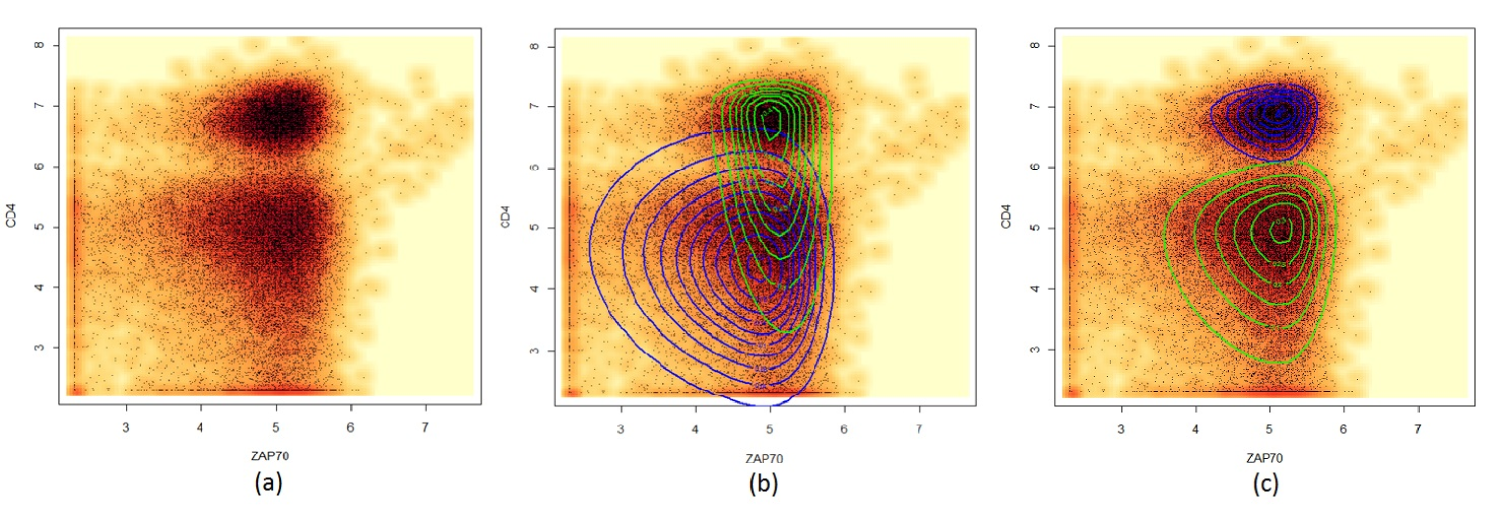
We consider a subset of the T-cell phosphorylation data collected by Maier et al. (2007). In the original data, blood samples from 30 subjects were stained with four fluorophore-labeled antibodies against CD4, CD45RA, SLP76(pY128), and ZAP70(pY292) before and after an anti-CD3 stimulation. In this example, we focus on a reduced subset of the data in two variables – CD4 and ZAP70. This bivariate sample (Figure 1) is apparently bimodal and exhibits asymmetric pattern. Hence we fit a two-component FM-MST model to the data. More specifically, the fitted model can be written as

f_{2}\left(\boldsymbol{y}_{j};\boldsymbol{\Psi}\right)=\pi_{1}f_{2}\left(\boldsymbol{y}_{j};\boldsymbol{\mu}_{1},\boldsymbol{\Sigma}_{1},\boldsymbol{\delta}_{1},\nu_{1}\right)+\left(1-\pi_{1}\right)f_{2}\left(\boldsymbol{y}_{j};\boldsymbol{\mu}_{2},\boldsymbol{\Sigma}_{2},\boldsymbol{\delta}_{2},\nu_{2}\right),

where

\boldsymbol{\mu}_{i}=\left(\mu_{i,1},\mu_{i,2}\right)^{T},\;\boldsymbol{\Sigma}_{i}=\left(\begin{array}[]{cc}\sigma_{i,11}&\sigma_{i,12}\\ \sigma_{i,12}&\sigma_{i,22}\end{array}\right),\boldsymbol{\delta}_{i}=\left(\delta_{i,1},\delta_{i,2}\right)^{T}(i=1,2).

For comparison, we include the fitting of a two-component mixture of skew $t$ -distributions from the skew-normal independent (SNI) family (Lachos, Ghosh, and Arellano-Valle, (2010)), hereafter named the FM-SNI-ST model. The estimated FM-SNI-ST density can be computed from the R package mixsmsn (Cabral, Lachos, and Prates, (2012)). Note that the MST distribution is different to the SNI-ST distribution since the skewing function is not of dimension one. Note also that the SNI-ST distribution is equivalent to the restricted MST distribution (5) after reparametrization. Moreover, under the FM-SNI-ST settings, the correlation structure of $\boldsymbol{Y}$ will also be dependent on the skewness parameter, whereas for the FM-MST distributions the covariance structure is not affected by $\boldsymbol{\delta}$ . The contours of the fitted SNI-ST and MST component densities are depicted in Fig 1(b) and Fig 1(c), respectively. To better visualize the shape of the fitted models, we display the estimated densities of each component instead of the mixture contours. It can be seen that the FM-MST model provides a noticeably better fit. From a clustering point of view, the FM-MST model also shows better performance as it is able to separate the two clusters correctly. Moreover, it adapts to the asymmetric shape of each cluster more adequately. Thus the superiority of FM-MST model is evident in dealing with asymmetric and heavily tailed data in this data set.

Refer to caption — Figure 1: Mixture modelling of a reduced subset of prephosphorylation T cell population. Bivariate skew $t$ -mixtures were fitted to the data restricted in two dimensions CD45 and ZAP70. (a) Hue intensity plot of the Lymphoma data set; (b) the contours of the component densities in the fitted two-component skew $t$ -mixture model FM-SNI-ST using the R package mixsmsn; (c) the fitted component contours of the two-component FM-MST model.

7.2 GvHD Data

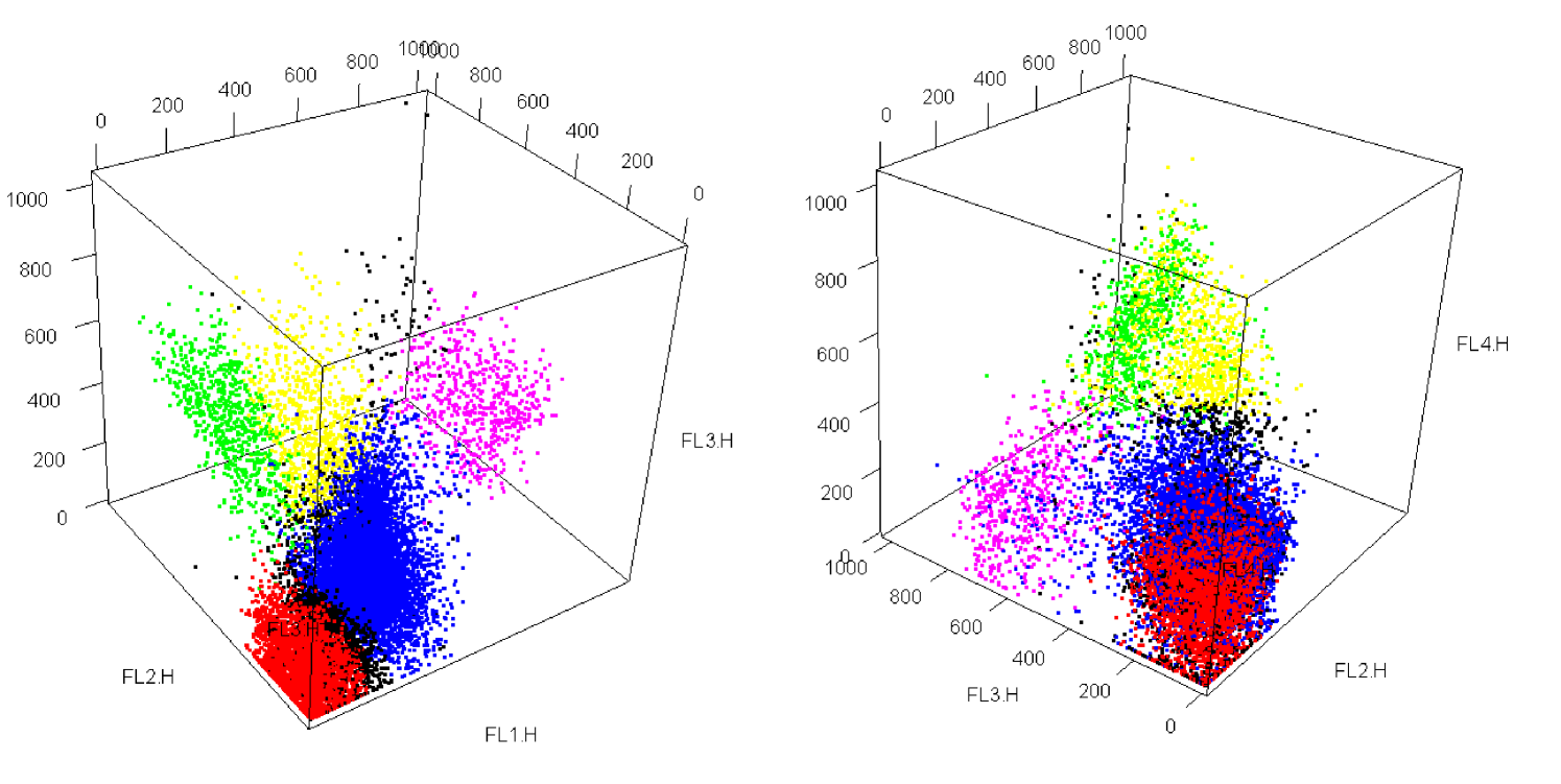
Our second example concerns a data set collected by Brinkman et al. (2007), where peripheral blood samples were collected weekly from patients following blood and bone marrow transplant. The original goal was to identify cellular signatures that can predict or assist in early detection of Graft versus Host Disease (GvHD), a common post-transplantation complication in which the recipient’s bone marrow was attacked by the new donor material. Samples were stained with four fluorescence reagents: CD4 FITC, CD8 $\beta$ PE, CD3 PerCP, and CD8 APC. Hence we fit a 4-variate FM-MST model to a case sample with a population of 13773 cells. The data set is shown in Figure 2, where cells are displayed in five different colours according to a manual expert clustering into five clusters. In addition, we include the results for the FM-SNI-ST model and the restricted MST mixture model introduced in Section 2.1 (equation 5), hereafter denoted by FM-RMST.

We compare the performance of the three models FM-MST, FM-SNI-ST, and FM-RMST in assigning cells to the expert clusters. Manual gating suggests there are five clusters in this case sample. Hence we applied the algorithm for the fitting of each model with $g$ predefined as $5$ . For a fair comparison, we started the three algorithms using the same initial values. The initial clustering is based on $k$ -means.The degrees of freedom are set to be identical for all components for the first iteration and assigned a relatively large value. A similar strategy was described in Lin (2010).

To assess the performance of these three algorithms, we take the manual expert clustering as being the ‘true’ class membership and we calculated the error rate of classification against this benchmark result with dead cells removed, measured by choosing among the possible permutations of class labels the one that gives the highest value.

As anticipated, the optimal clustering result was given by the FM-MST model. It achieved the lowest misclassification rate. The FM-SNI-ST model has a higher number of misallocations. The FM-RMST model has a disappointing performance in terms of clustering. Its error rate is almost double that of its competitors. It is worth pointing out that both the FM-MST and FM-RMST models have 99 free parameters, while the FM-SNI-ST model has 95 parameters. It is evident that these two restricted models have inferior performance. This reveals some evidence of the extra flexibility offered by the more general FM-MST model.

Table 1: Clustering error rates for various multivariate skew

t

mixture models on the GvHD data set.

Model	Error rate	Number of free parameters
FM-MST	0.0875	99
FM-SNI-ST	0.13078	95
FM-RMST	0.20700	99

7.3 AIS Data

We now illustrate the computational efficiency of our exact implementation of the E-step of the EM algorithm as in Section 5. We denote this version of the EM algorithm with the exact E-step as EM-exact. In addition, we consider the EM alternative with a Monte Carlo (MC) E-step as given by Lin (2010), which is denoted by EM-MC. Since both models are based on the same characterization of the multivariate skew $t$ -distribution defined by Sahu et al. (2003), it is appropriate to compare their computation time. We assess their time performance on the well-analyzed Australian Institute of Sport (AIS) data, which consists of $p=13$ measurements made on $n=202$ athletes. As in Lin (2010), we limit this illustration to a bivariate subset of two variables – body mass index (BMI) and the percentage of body fat (Bfat). As noted by Lin (2010), these data are apparently bimodal. Hence a two-component mixture model is fitted to the data set.

A summary of the results are listed in Table 2. Also reported there are the values of the log-likelihood, the Akaike information criterion (AIC) (Akaike, 1974) and the Bayesian information criterion (BIC) (Schwarz, 1978) defined by

\mbox{AIC}=2m-2L\left(\boldsymbol{\Psi}\right)\;\mbox{and}\;\mbox{BIC}=m\log n-2L\left(\boldsymbol{\Psi}\right),

(41)

respectively, where $L\left(\boldsymbol{\Psi}\right)$ is the value of the log likelihood at $\boldsymbol{\Psi}$ , $m$ is the number of free parameters, and $n$ is the sample size. Models with smaller AIC and BIC values are preferred when comparing different fitted results. The best value from each criterion are highlighted in bold font in Table 2. For this illustration, the EM-MC E-step is undertaken with $50$ random draws as recommended by Lin (2010). Note that the degrees of freedom is not restricted to be the same for the two components. The gender of each individual in this data set is also recorded, thus enabling us to evaluate the error rate of binary classification for the two methods.

Not surprisingly, the model selection criteria favour the EM-exact algorithm. Not only did it achieve lower AIC and BIC values, the computation time is remarkably lower than its competitor. It is more than five times faster than the EM-MC alternative.

Table 2: Computation time and clustering error rates for two different implementations of the EM algorithm for the multivariate skew

t

mixture models on the AIS data set. For EM-exact, the E-step is implemented exactly as described in Section 5. As an alternative, the EM algorithm was implemented with a Monte Carlo E-step, EM-MC, as in Lin (2010). Time is measured in seconds.

Model	EM-exact		EM-MC
Component	1	2	1	2
$\pi$	0.44	0.56	0.59	0.41
$\mu_{i1}$	19.74	21.83	19.89	22.47
$\mu_{i2}$	15.99	5.89	15.50	7.30
$\Sigma_{i,11}$	3.03	3.16	2.96	3.23
$\Sigma_{i,12}$	7.71	0.54	6.17	1.34
$\Sigma_{i,22}$	2.36	0.11	25.80	2.14
$\delta_{i1}$	3.34	1.44	2.72	0.71
$\delta_{i2}$	3.15	3.76	2.22	1.13
$\nu$	42.05	3.82	23.98	25.93
$L\left(\boldsymbol{\Psi}\right)$	-1077.257		-1088.066
AIC	2188.514		2207.956
BIC	2244.755		2264.197
error rate	0.0792		0.0891
time	64.63		349.9

8 Computation Time and Accuracy for E-step

We now proceed to two interesting experiments for evaluating the computational cost and accuracy of using the EM-exact and EM-MC algorithms on high-dimensional data. As pointed out previously, the main computational cost for EM-exact is evaluating the multivariate $t$ -distribution function. Calculation of the first two moments of a $p$ -variate truncated $t$ -distribution requires the evaluation of two $T_{p}(\cdot)$ functions, $p$ evaluations of $T_{p-1}(\cdot)$ , and $\textstyle\frac{1}{2}p(p-1)$ evaluations of $T_{p-2}(\cdot)$ . Hence, the computation time will increase substantially with the number of dimensions. However, with the EM-exact algorithm, accuracy can be compromised for time.

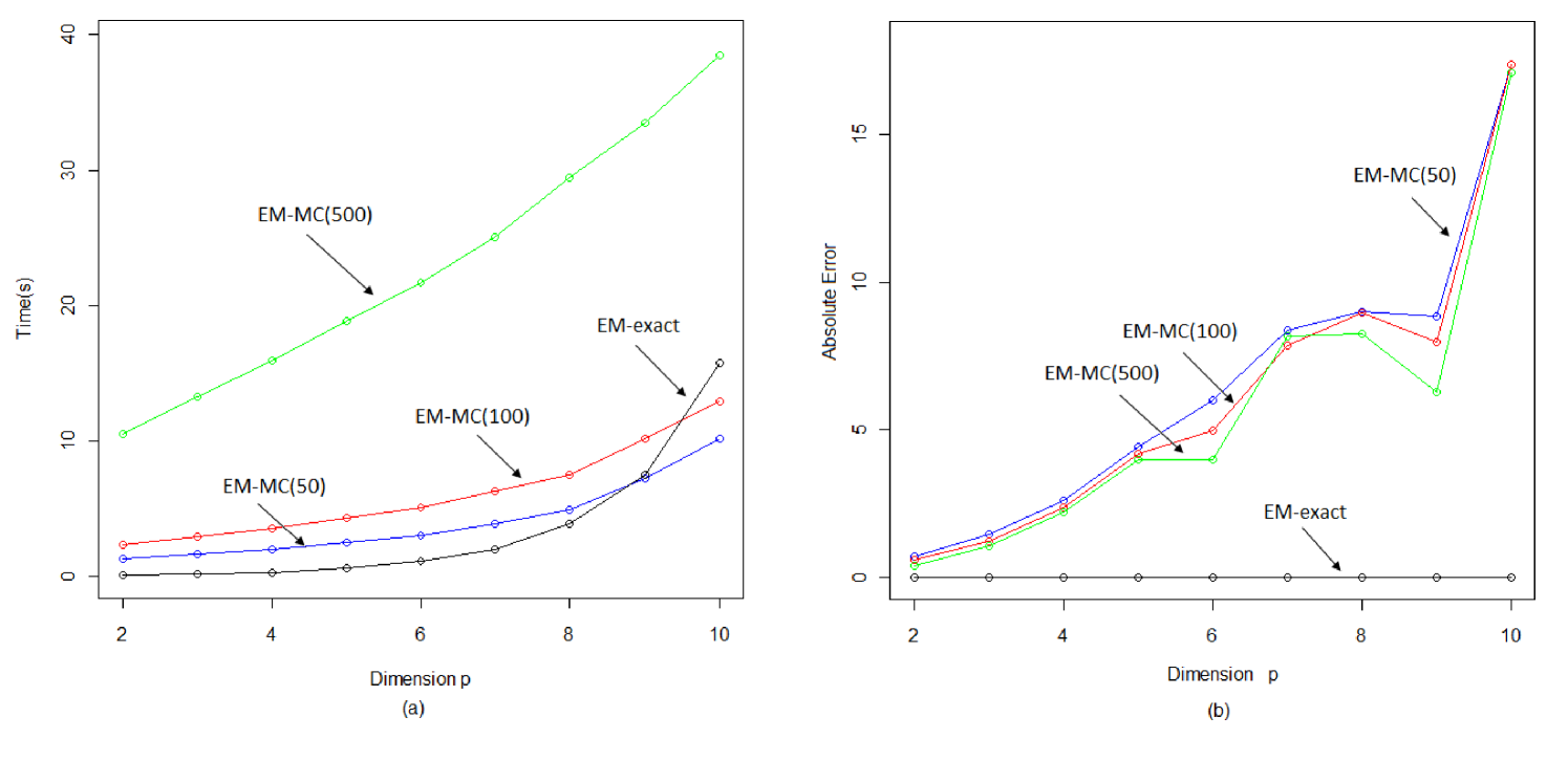
We sampled 100 data from a Brain Tumor dataset supplied by Geoff Osborne from the Queensland Brain Institute at the University of Queensland. In both experiments we varied the dimension $p$ of the sample. The graph in Figure 3(a) shows the typical CPU time per each E-step iteration for various dimensions $p$ of the data; EM-MC $(m)$ represents the EM-MC algorithm with $m$ random draws using the Gibbs sampling approach described in Lin (2010). It is worth noting that in both experiments EM-exact is evaluated with a default tolerance of at least $10^{-6}$ . As seen in Figure 3, EM-exact is the fastest among the four versions of the E-step for low dimensions. For example, at $p=2$ , EM-exact at least 25 times faster than EM-MC(50). It is important to note that although EM-MC(50) is slightly faster than EM-exact at higher dimensions, EM-exact produces results to a significantly higher accuracy, while EM-MC requires a large number of draws to achieve comparable results. We note that in our simulations, for example, at $p=7$ , 50 draws is insufficient to achieve acceptable estimates. Preliminary results suggests that at least 500 draws is required to generate reasonable approximations when $p$ is greater than 6. In this case, EM-exact is at least ten times quicker. Furthermore, EM-exact also has an additional advantage over the EM-MC alternative in that its results are reproducible.

To compare the accuracy of the EM-exact and EM-MC algorithms, we compute the total absolute error against the baseline EM-exact with a maximum tolerance of $10^{-18}$ . For each of the EM-MC $(m)$ algorithms, the average total absolute error of 100 trials is used. For EM-exact, the default tolerance is set to $10^{-6}$ . The results are shown in Figure 3(b). Not surprisingly, the absolute error of the EM-MC algorithm is significantly higher than that of the EM-exact algorithm. It can be observed that the absolute error is very high even for EM-MC(500). At $p=10$ , for example, EM-exact is at least 30000 times more accurate and takes less than half the time required for EM-MC(500).

It is important to emphasize that as the dimension $p$ of the data increases, EM-MC requires considerably more draws to provide a comparable (and acceptable) level of accuracy as EM-exact, which can be computationally intensive. Hence we advocate the use of EM-exact, especially for applications involving high dimensional data.

9 Concluding Remarks

We have described an exact EM algorithm for evaluating the parameters of a general multivariate skew $t$ -mixture model. This model has a more general characterization than various alternative versions of the skew $t$ -distribution available in the literature and hence offers greater flexibility in capturing the asymmetric shape of skewed data.

Our proposed method is based on reduced analytical expressions for the E-step conditional expectations, which can be formulated in terms of the first and second moments of a multivariate truncated $t$ -distribution. The latter can then be expressed further in terms of the distribution function of the multivariate central $t$ -distribution for which fast algorithms capable of producing highly accurate results already exist. It is demonstrated to have a marked advantage over the EM algorithm with a Monte Carlo E-step. To achieve comparable accuracy to that of the EM algorithm with the E-step implemented using the above numerical approach, the version of the algorithm with a Monte Carlo E-step would require a large number of draws, which would be computationally expensive.

Acknowledgments

This work is supported by a grant from the Australian Research Council. Also, we would like to thank Professor Seung-Gu Kim for comments and corrections, and Dr Kui (Sam) Wang for his helpful discussions on this topic.

References

[1] H. Akaike. A new look at the statistical model identification. Automatic Control, 19:716–723, 1974.
[2] R.B. Arellano-Valle, H. Bolfarine, and V.H. Lachos. Bayesian inference for skew-normal linear mixed models. Journal of Applied Statistics, 34(6):663–682, 2007.
[3] A. Azzalini. A class of distributions which includes the normal ones. Scandinavian Journal of Statistics, 12:171–178, 1985.
[4] A. Azzalini and A Dalla Valle. The multivariate skew-normal distribution. Biometrika, 83(4):715–726, 1996.
[5] J. D. Banfield and A. Raftery. Model-based gaussian and non-gaussian clustering. Biometrics, 49:803–821, 1993.
[6] K. E. Basford, D. R. Greenway, G. J. McLachlan, and D. Peel. Standard errors of fitted means under normal mixture. Computational Statistics, 12:1–17, 1997.
[7] R. M. Basso, V. H. Lachos, C. R. B. Cabral, and P. Ghosh. Robust mixture modeling based on scale mixtures of skew-normal distributions. Computational Statistics and Data Analysis, 54:2926–2941, 2010.
[8] M. D. Branco and D. K. Dey. A general class of multivariate skew-elliptical distributions. Journal of Multivariate Analysis, 79:99–113, 2001.
[9] R. Brinkman, M. Gaspareto, S.-J. Lee, A. Ribickas, J. Perkins, W. Janssen, R. Smiley, and C. Smith. High content flow cytometry and temporal data analysis for defining a cellular signature of graft versus host disease. Biological of Blood and Marrow Transplantation, 13:691–700, 2007.
[10] C.S. Cabral, V.H. Lachos, and M.O. Prates. Multivariate mixture modeling using skew-normal independent distributions. Computational Statistics and Data Analysis, 56:126–142, 2012.
[11] A.P. Dempster, N. M. Laird, and D. Rubin. Maximum likelihood from incomplete data via the em algorithm. Journal of Royal Statistical Society , Series B, 39:1–38, 1977.
[12] B. S. Everitt and D. J. Hand. Finite Mixture Distributions. Chapman and Hall, London, 1981.
[13] C. Fraley and A. E. Raftery. How many clusters? which clustering methods? answers via model-based cluster analysis. Computer Journal, 41:578–588, 1999.
[14] A Genz and F. Bretz. Methods for the computation of multivariate t-probabilities. Journal of Computational and Graphical Statistics, 11:950–971, 2002.
[15] P. J. Green. On use of the em algorithm for penalized likelihood estimation. Journal of the Royal Statistical Society B, 52:443–452, 1990.
[16] A. K. Gupta. Multivariate skew- $t$ distribution. Statistics, 37:359–363, 2003.
[17] S. Kotz and S. Nadarajah. Multivariate t Distributions and Their Applications. Cambridge University Press, Cambridge, 2004.
[18] V. H. Lachos, P. Ghosh, and R. B. Arellano-Valle. Likelihood based inference for skew normal independent linear mixed models. Statistica Sinica, 20:303–322, 2010.
[19] T. I. Lin. Robust mixture modeling using multivariate skew $t$ distribution. Statistics and Computing, 20:343–356, 2010.
[20] T. I. Lin, J. C. Lee, and W. J. Hsieh. Robust mixture modeling using the skew- $t$ distribution. Statistics and Computing, 17:81–92, 2007.
[21] T. I. Lin, J. C. Lee, and S. Y. Yen. Finite mixture modelling using the skew normal distribution. Statistica Sinica, 17:909–927, 2007.
[22] B. G. Lindsay. Mixture Models: Theory, Geometry, and Applications. NSF-CBMS Regional Conference Series in probability and Statistics, Volume 5, Institute of Mathematical Statistics, Hayward, CA, 1995.
[23] L. M. Maier, D. E. Anderson, P. L. De Jager, L.S. Wicker, and D. A. Hafler. Allelic variant in ctla4 alters t cell phosphorylation patterns. Proceedings of the National Academy of Sciences of the United States of America, 104:18607–18612, 2007.
[24] G. J. McLachlan and K. E. Basford. Mixture Models: Inference and Applications. Marcel Dekker, New York, 1988.
[25] G. J. McLachlan and T. Krishnan. The EM Algorithm and Extensions. Wiley-Interscience, Hokoben, N. J., 2nd edition, 2008.
[26] G. J. McLachlan and D. Peel. Finite Mixture Models. Wiley Series in Probability and Statistics, 2000.
[27] G.J. McLachlan and D. Peel. Robust cluster analysis via mixtures of multivariate $t$ -distributions. In A. Amin, D. Dori, P. Pudil, and H. Freeman, editors, Lecture Notes in Computer Science, volume 1451, pages 658–666. Springer-Verlag, Berlin, 1998.
[28] A. O’Hagan. Bayes estimation of a convex quadratic. Biometrika, 60:565–571, 1973.
[29] A. O’Hagan. Moments of the truncated multivariate- $t$ distribution. 1976.
[30] S. Pyne, X. Hu, K. Wang, E. Rossin, T.-I. Lin, L. M. Maier, C. Baecher-Allan, G. J. McLachlan, P. Tamayo, D. A. Hafler, P. L. De Jager, and J. P. Mesirow. Automated high-dimensional flow cytometric data analysis. PNAS, 106:8519–8524, 2009.
[31] S.K. Sahu, D.K. Dey, and M.D. Branco. A new class of multivariate skew distributions with applications to bayesian regression models. The Canadian Journal of Statistics, 31:129–150, 2003.
[32] G. Schwarz. Estimating the dimension of a model. Annals of Statistics, 6:461–464, 1978.
[33] D. M. Titterington, A. F. M. Smith, and U. E. Markov. Statistical Analysis of Finite Mixture Distributions. Wiley, New York, 1985.

On the fitting of mixtures of multivariate skew tt-distributions via the EM algorithm

Abstract

1 Introduction

2 Preliminaries

2.1 The Multivariate Skew tt-Distribution

2.2 The truncated multivariate tt-distribution

3 ML Estimation for the MST Distribution

3.1 M-step

4 The Multivariate Skew tt-Mixture Model

5 ML Estimation for FM-MST Distributions

6 The Empirical Information Matrix

7 Examples

7.1 Lymphoma Data

7.2 GvHD Data

7.3 AIS Data

8 Computation Time and Accuracy for E-step

9 Concluding Remarks

Acknowledgments

References

On the fitting of mixtures of multivariate skew $t$ -distributions via the EM algorithm

2.1 The Multivariate Skew $t$ -Distribution

2.2 The truncated multivariate $t$ -distribution

4 The Multivariate Skew $t$ -Mixture Model