On the implied volatility of Inverse options under stochastic volatility models
Abstract
In this paper, we study the short-time behavior of at-the-money implied volatility for inverse European options with a fixed strike price. The asset price is assumed to follow a general stochastic volatility process. Using techniques from Malliavin calculus, such as the anticipating Itô’s formula, we first compute the implied volatility of the option as its maturity approaches zero. Next, we derive a short-maturity asymptotic formula for the skew of the implied volatility, which depends on the roughness of the volatility model. We also demonstrate that our results can be easily extended to Quanto-Inverse options. We apply our general findings to the SABR and fractional Bergomi models and provide numerical simulations that confirm the accuracy of the asymptotic formula for the skew. Finally, we present an empirical application using Bitcoin options traded on Deribit, showing how our theoretical formulas can be applied to model real market data for such options.
Keywords: Inverse European options, stochastic volatility, crypto derivatives, Malliavin calculus, implied volatility
1 Introduction
Over the last several decades, option pricing models have been developed for conventional assets such as stocks, bonds, interest rates, and foreign currencies. Today, cryptocurrency derivatives, financial contracts whose value depends on an underlying cryptocurrency asset, have emerged as a new class of securities that have garnered significant attention. A key peculiarity of crypto derivatives is how one defines a cryptocurrency: Is it a security, a currency, or a commodity? With regard to options, the answer to this question affects the pricing methodology. A detailed discussion on this topic can be found in Alexander et al. [1]. Unfortunately, there is no clear legal answer to this question; see Bolotaeva et al. [12]. However, a closer examination of the issue leads to the following conclusions.
Cryptocurrency (at least Bitcoin and Ethereum) cannot be considered a security, as it is fully decentralized, and no central authority controls its issuance, whereas securities are issued by a central authority. Furthermore, cryptocurrencies cannot be treated as conventional (fiat) currencies. A key question is whether they preserve the fundamental characteristics of money. Although cryptocurrencies can occasionally be used to buy and sell goods, they are not widely accepted as a means of payment. Furthermore, historical data shows the extreme volatility of cryptocurrencies, leading to the conclusion that their purchasing power is not stable enough over time, and therefore they cannot serve as a store of value. In contrast, Central Bank Digital Currency addresses the volatility issue by controlling the issuance. Finally, although some companies may accept cryptocurrencies as payment, most still use traditional currencies to measure the value of goods and services. For further discussion on the similarities between cryptocurrencies and regular currencies, see Hazlett and Luther [20] and Ammous [10].
On the other hand, if we consider the classical Garman and Kohlhagen [16] foreign exchange (FX) pricing model, the construction of the delta-hedged portfolio for FX options is conceptually different from regular options, as we cannot buy and sell units of the FX spot rate. Instead, hedging is done by buying and selling units of the underlying foreign bond. This difference fundamentally undermines the idea of pricing crypto options using FX models, as cryptocurrencies can be bought and sold in a manner similar to regular tradable assets.
Alternatively, some people consider Bitcoin to be digital gold, but how similar is it to the actual commodity? In Goutteet al. [17], the authors define the following characteristics of hard commodities: they are costly to mine or extract, storable, not controlled by any single government or institution in terms of global supply, demand, or price, and they have intrinsic value, which means that they can be consumed or used as inputs in the production of other goods. The first three properties are naturally satisfied by Bitcoin, but the fourth remains debatable. As a result, we cannot conclusively classify crypto as a commodity. For a more detailed discussion, see Ankenbrand and Bieri [11] and Gronwald [18]. Finally, Dyhrberg [15] provides an empirical analysis using GARCH models for Bitcoin volatility to explore whether Bitcoin is more similar to gold or the US dollar.
The aim of this paper is to solve the pricing problem of crypto options using only the payoff function. A natural way to define the payoff of crypto options is through Inverse options, which are settled in cryptocurrency rather than fiat currency. We will focus on the case of an Inverse European call, whose payoff is given by:
where , denotes the price of Bitcoin in US dollars at maturity and is a fixed strike. In simple terms, if the option becomes in-the-money, the payoff is made in cryptocurrency rather than fiat currency.
Inverse European options are the only type of options traded on the Deribit exchange, which controls over 80 percent of the global crypto options market. For example, on June 10, 2023, the open interest in Bitcoin options on Deribit was 7.5 billion, while the closest competitors, OKX and Binance, had open interest of 0.5 billion and 0.17 billion, respectively. As a result, accurately pricing and hedging Inverse European options is crucial from a practical standpoint. However, this is quite challenging due to the mechanics of the Deribit exchange. Deribit does not allow fiat currency, and all options are margined in cryptocurrency. This is particularly beneficial for professional crypto traders. For instance, consider a crypto hedge fund or a crypto market maker, businesses that deal exclusively with crypto assets. It is natural for them to manage their trading books in cryptocurrency rather than fiat currency. While they are exposed to cryptocurrency depreciation risk, it is easier to manage this risk at the book level rather than on a trade-by-trade basis. This is one of the key reasons for the development of Inverse European options.
The literature on crypto derivatives is still relatively new but has been gaining increasing attention from researchers. For example, Alexander et al. [1] price Inverse European options under the constant volatility Black-Scholes model. Matic et al. [23] study empirical hedging of Inverse options under different stochastic volatility models. Alexander et al. [2] use a delta adjusted for skew to hedge Inverse options under constant and local volatility. Hou et al. [21] price Inverse options under stochastic volatility models with correlated jumps. Finally, Siu and Elliott [27] use the SETAR-GARCH model to model Bitcoin return dynamics.
In this paper, we study the behavior of implied volatility for Inverse European options under general stochastic volatility models. Specifically, we provide general sufficient conditions on a stochastic volatility model to derive short-time maturity asymptotic formulas for the at-the-money level and the skew of the implied volatility of Inverse options. We then apply these results to two well-known models: the SABR and fractional Bergomi models.
The main tool for proving these results is the anticipating Itô’s formula from Malliavin calculus; see Appendix A for an introduction to this topic. The first step is to apply this formula using a similar approach to Alòs [3], in order to derive a decomposition formula for the option price; see Theorem 2. This approach is also used in Alòs et al. [7] for jump-diffusions with stochastic volatility. In that paper, the short-time limit of the implied volatility skew for European calls is also derived, which corresponds to the second step of our paper. This approach has been further developed in other contexts. Recently, Alòs et al. [5] applied this methodology to VIX options, and Alòs et al. [8] extended it to Asian options. These two papers demonstrate how studying Asian or VIX options under stochastic volatility reduces to studying European-type options, where the underlying is represented by a stochastic volatility model with a modified volatility process that depends on maturity.
In the present paper, we extend the methodology outlined above to Inverse European calls. The main novelty, compared to the papers mentioned, is the following.
-
•
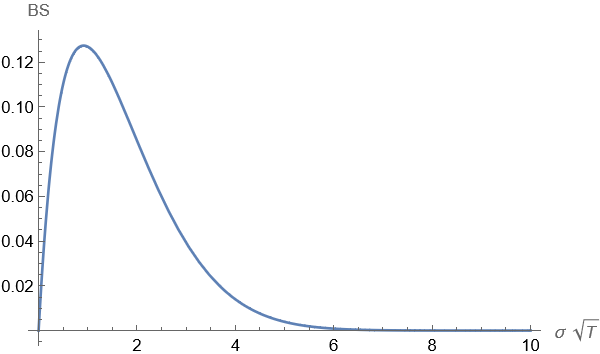
To the best of our knowledge, we are the first to provide a rigorous analytical study of the asymptotic behavior of the implied volatility of Inverse European options under fractional and stochastic volatility models. When dealing with Inverse options, the Black-Scholes formula differs from the classical one, so our results cannot be directly derived from existing literature. Instead, we work with the Black-Scholes formula for Inverse European calls under constant volatility, as obtained in Alexander et al. [1]. This formula turns out to be a non-monotonic function (see Figure 8), meaning its inverse is not uniquely defined, which complicates computations since implied volatility is defined as the inverse of the Black-Scholes formula. We overcome this challenge by noting that for sufficiently small maturities, which is the case studied in this paper, the function is strictly monotonic. However, the inverse is not explicit as in the classical Black-Scholes case, so a careful study of its behavior and derivatives is required, as shown in Appendix B.
-
•
Our formulas can be applied to general stochastic and fractional volatility models. We provide numerical simulations using the SABR and fractional Bergomi models. Additionally, we present an empirical example with Bitcoin options to demonstrate how the results of this paper can be used to model real market data for such options, which have become increasingly popular in financial markets, as discussed at the beginning of this introduction.
Understanding the behavior of the implied volatility of Inverse options is crucial for hedging purposes and can also be used to derive approximation formulas for their price, as mentioned at the end of Section 2. In a world with a flat implied volatility surface, one could simply use the Black-Scholes delta to replicate the derivative payoff. However, in the presence of implied volatility skew, the classical Black-Scholes hedge will not be accurate. The correct approach is to use the Black-Scholes delta with a correction based on the implied volatility skew. In our empirical example, we focus on the fractional Bergomi model.
One of the key parameters in this model is the Hurst exponent . Its value determines the skew that can be reproduced from market data. Since different markets exhibit different behaviors, we expect to see varying values of that best fit the observed data. For example, in equity markets, the implied volatility skew exhibits a blow-up, which can be reproduced with , corresponding to rough volatility See, for instance, Cont and Das [14]. In our case, we find that best fits our market data and produces zero skew.
Additionally, our analysis allows us to derive the same formulas for Quanto-Inverse European options, whose payoff is given by:
where is a fixed exchange rate. From a mathematical perspective, Quanto-Inverse options do not differ significantly from Inverse options. In particular, as shown in Section 2, the implied volatility level and skew of both options are equal up to a factor of , so it is sufficient to study Inverse options. However, from a practical perspective, Inverse and Quanto-Inverse options differ, as they are traded on different markets. Unlike Inverse options, which are available to the general public, Quanto-Inverse options are over-the-counter derivatives.
The paper is organized as follows: Section 2 presents the problem statement and the main result, Theorem 1, where the at-the-money implied volatility level is derived in (6) and the skew in (7). The intermediate steps leading to the proof of this theorem are provided in Section 3. Specifically, Theorem 2 enables us to obtain (6), and Propositions 1 and 2 are crucial for deriving (7). Note that Proposition 1 relies on (6). The proof of Theorem 1 is provided in Section 4. Section 5 presents a numerical study for the SABR and fractional Bergomi models, along with an empirical application to the implied volatility of Bitcoin options.
2 Statement of the problem and main results
Consider the following model for the asset price on the time interval
| (1) |
where is fixed and , , and are three standard Brownian motions on defined on the same risk-neutral complete probability space . We denote by the expectation with respect to . For simplicity, we assume that the interest rate is zero, see for instance in Alòs et al. [5]. We assume that and are independent and is the correlation coefficient between and .
We consider the following hypotheses on the volatility process :
Hypothesis 1.
The process is square integrable, adapted to the filtration generated by , a.s. positive and continuous, and satisfies that for all ,
for some positive constants and .
Hypothesis 2.
For all there exist and such that for all ,
Hypothesis 3.
For all , (see Appendix A for the definition of this space).
Hypothesis 4.
There exists and for all there exist constants such that for a.e.,
| (2) |
and
| (3) |
where denotes the Malliavin derivative defined in Appendix A.
We observe that when the volatility is constant, the model (1) is the usual Black-Scholes model. We also observe that although the volatility can be driven by a fractional Brownian motion (see Section 5.2), we are assuming that the volatility is not a traded asset. Thus, there exists a risk-neutral probability and there are no arbitrage opportunities (see Comte and Renault [13]). Moreover, if and denote the values of an Inverse European call and a Quanto Inverse European call options with fixed strike , respectively, we have that
and
where is a fixed exchange rate. Recall that denotes the expectation under a risk-neutral probability . Note that as in [7], we assume that the market selects a unique risk-neutral measure under which these derivative contracts are priced.
Notice that the difference between and arises from the currency in which the options are quoted. In our case, represents the crypto price of the option, while represents the dollar value of the option.
We denote by the Black-Scholes price of an Inverse European call option with time to maturity , log-underlying price , log-strike price and volatility . Then, it is well-known that (see Alexander et al. [1]),
where is the cumulative distribution function of a standard normal random variable. Moreover, the Black-Scholes price for a Quanto Inverse European call is given by .
One can easily check that the Black-Scholes price satisfies the following PDE
| (4) |
Moreover, one can also check that the classical relationship between the Gamma, the Vega and the Delta holds, that is,
| (5) |
As in Alòs [3], we consider the log price , which satisfies
Next, we observe that, as , the price of an Inverse call option can be written as
and by continuity we have . In particular, . Notice that . This implies that the implied volatility level and skew of Inverse and Quanto Inverse European call options are equal up to the factor . Hence, we will only state the main results of this paper for the Inverse options.
We define the at-the-money implied volatility (ATMIV) of an Inverse European call option as the quantity satisfying
where . That is, . As it is shown in Appendix B, this inverse is only well-defined for sufficiently small, which is the case we are studying in this paper. Precisely, the aim of this paper is to apply the Malliavin calculus techniques developed in Alòs [3] in order to obtain formulas for
under the general stochastic volatility model (1).
The main results of this paper are given in the following theorem.
Theorem 1.
Assume Hypotheses 1-4. Then,
| (6) |
Moreover,
| (7) | ||||
provided that both limits exist.
We observe that when prices and volatilities are uncorrelated then the short-time skew equals to zero. Observe also that since the term is of order (see Hypothesis 4), the quantity multiplying the term of the right hand side of (7) is bounded by . In particular, its limit is if . This suggests that, in the case , we need to multiply by in order to obtain a finite limit. See the examples in Section 5.
The results of Theorem 1 can be used in order to derive approximation formulas for the price of an Inverse and Quanto Inverse European call options. Notice that, as
by Taylor’s formula we can use the approximations
Of course, this approximation is only linear, and one would expect to obtain better results if one has a short maturity asymptotic formula for the curvature . The short-time maturity asymptotics for the at-the-money curvature of the implied volatility for European calls under general stochastic volatility models is computed in Alòs and León [6]. A Taylor expansion for short maturity asymptotics for Asian options when the underlying asset follows a local volatility model is obtained in Pirjol and Zhu [26]. In our setting, computing the curvature is more challenging and we leave it for further work.
3 Preliminary results
In this section, we provide closed-form decomposition formulas for the price and the ATMIV skew of an Inverse call option under the stochastic volatility model (1).
We begin with the following preliminary lemma. For the standard European call option case, see Lemma 6.3.1 in Alòs et al. [5].
Lemma 1.
Assume Hypothesis 1. Then, for all there exist positive constants , and such that for all ,
| (8) | ||||
| (9) | ||||
| (10) |
where and
.
Proof.
Using Hypothesis 1, the fact that for all and the function is bounded, and that it is easy to see that the first term is bounded by .
For the second term, we use the fact that the function Erfc is bounded and that has bounded moments of all orders by Hypothesis 1. This completes the proof of (8).
We next prove (9). Straightforward differentiation gives
Then, due to Hypothesis 1, we get that
where .
Hence, using the fact that for all and the function is bounded and , we conclude that (9) holds true.
Finally, we have that
and the same argument as above allows us to complete the proof (10), and thus the proof of the Lemma. ∎
The first result of this section is the decomposition of the price of inverse options. The proof follows exactly the same lines as Theorem 4.2 in Alòs et al. [7]. See also Theorem 6 in Alòs [3] and Theorem 26 in Alòs et al. [5]. Note that the derivatives of the Black-Scholes formula for inverse options satisfy the same equations, (4) and (5), which is the key ingredient of the proof, together with the anticipating Itô’s formula. For completeness, we provide a sketch of the proof, as the derivatives of the Black-Scholes formula are different. Thus, Lemma 1 (instead of Lemma 2 in [7]) is needed to verify that all the integrals are well-defined.
Theorem 2.
Assume Hypotheses 1-4. Then, the following relation holds
where recall that .
Proof.
Since , the law of one price leads us to the conclusion that . Then, we apply the anticipating Itô’s formula of Theorem 4 in Appendix A to the function , observing that with for . That is, . Then, we get that
By adding and subtracting to the expression above we get that
Notice that the second term in the above expression is equal to zero due to formula (4). Finally, using equation (5) and taking expectation, we complete the proof. Observe that by Lemma 1 and Hypotheses 1-4 all expectations are finite. In fact, using Cauchy-Schwarz inequality, and Hypotheses 1 and (2), we get that
We also observe that since the function and its derivatives are not bounded, exactly the same truncation argument of Theorem 4.2 in [7] can be used here in order to apply Theorem 4 in Appendix A. ∎
We next derive an expression for the ATMIV skew of an Inverse European call option under the stochastic volatility model (1). The proof follows similarly to Theorem 4.2 in Alòs et al. [7], but with the use of properties (12) and (13) of the Black-Scholes function for Inverse options, which differ from the standard Black-Scholes function.
Proposition 1.
Assume Hypotheses 1-4. Then,
| (11) | ||||
where , provided that both limits exist.
Proof.
Since , the following equation holds
On the other hand, using Theorem 2, we get that
Notice that by dominated convergence, we have that
where
| (12) |
Combining the above equations, we find that the volatility skew is equal to
Furthermore, using (12) and Theorem 2 we obtain that
Straightforward differentiation gives us the following expression
| (13) |
By (6), . Moreover, by continuity, we have that . Thus, . Thus, since , we conclude that
which completes the proof. ∎
To compute the limit of the skew slope of the ATMIV, we need to identify the leading-order terms of the numerator in equation (11). The following decomposition formula will be crucial in achieving this goal. The proof follows similarly to that in Alòs et al. [7]. For completeness, we provide a sketch of the proof.
Proposition 2.
Assume Hypotheses 1-4. Then,
where and .
Proof.
Applying Theorem 4 to the function and recalling that , we obtain
By adding and subtracting the term to the expression above we get that
Next, equations (4) and (5) imply that
Finally, taking expectations and noticing that by Lemma 1 and Hypotheses 1-4 all expectations are finite, we complete the desired proof. Remark that as for Theorem 2, the same truncation argument as in [7] can be used in order to apply Theorem 4 in Appendix A. ∎
4 Proof of Theorem 1
4.1 Proof of (6) in Theorem 1: ATMIV level
This section is devoted to the proof of (6) in Theorem 1. The proof follows similar ideas to those in Alòs and Shiraya [9], but a detailed study of the inverse of the Black-Scholes function for Inverse options is required, which is provided in Appendix B.
4.1.1 The uncorrelated case
We observe that as , the two Brownian motions and are independent. Thus, and is a martingale under the probability measure with respect to filtration . By the martingale representation theorem, there exists a square integrable and -adapted process such that
Clark-Ocone-Haussman formula (Theorem 3) gives us the following representation,
Then, a direct application of the classical Itô’s formula implies that
where and denote, respectively, the first and second derivatives of with respect to .
4.1.2 The correlated case
Using similar ideas as in the uncorrelated case we get that
where .
Then, a direct application of Itô’s formula gives us
By (8), we have that . Moreover, using the Lemma 2 in Appendix B we have that for sufficiently small . Therefore, using Hypotheses 1 and 4 and Cauchy-Schwarz inequality, we get that
Thus, . Finally, using (14) we conclude the proof of (6) in the correlated case.
4.2 Proof of (7) in Theorem 1: ATM implied volatility skew
We start by analysing the second term in (15). Using Hypotheses 1 and 4, (10) and Cauchy-Schwarz inequality, we get that
Hypothesis 1 implies that
Next, Hypotheses 1 and 4 together with Cauchy-Schwarz inequality yield to
Then, using the computations above together with (9), we get that
Finally, using the expression (13), we conclude that the limits of the two terms on the right-hand side of (15) are zero. Therefore, appealing again to (13), we conclude that
where
and
Notice that
Hence, using Hypotheses 1-4 and Cauchy-Schwarz inequality, we get that
Therefore, appealing to the Lebesgue dominated convergence theorem, we conclude the proof of (7).
5 Numerical analysis
In this section, we justify Theorem 1 with numerical simulations. Note that the SABR and fractional Bergomi models do not satisfy Hypothesis 1. However, a truncation argument justifies the application of Theorem 1, similar to the approach in Alòs and Shiraya [9] and Alòset al. [8]. See Appendix C for the details.
5.1 The SABR model
We consider the SABR stochastic volatility model (see Haganet al. [19]) with a skewness parameter equal to 1, which is the most common case from a practical point of view. This corresponds to equation (1), where denotes the forward price of the underlying asset and
where is the volatility of volatility.
For , we have and . Therefore, applying Theorem 1 we conclude that (see Appendix C)
| (16) | ||||
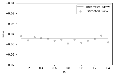
Observe that from equation (16), we can infer how the parameters of the SABR model influence the value of the ATM implied volatility skew. Firstly, the skew has a finite value, and its behavior depends on , the correlation between the underlying asset and its volatility, and , the volatility of volatility. Therefore, the sign of the skew is fully determined by the sign of . Furthermore, the magnitude of the skew is directly proportional to the parameters of the SABR model.
We next proceed with some numerical simulations using the following parameters
Observe that the maturity chosen for the simulations, , is equivalent to half a day, which is realistic, as the shortest maturity options on crypto exchanges are typically daily options.
To estimate the price of the Inverse European call option, we use antithetic variates. The price estimate is calculated as follows:
| (17) | ||||
where and the subscript denotes the value of the call option computed on the antithetic trajectory of a Monte Carlo path.
To recover the implied volatility, we use Brent’s method, which combines the bisection, secant, and inverse quadratic interpolation methods, ensuring guaranteed convergence to a root. This method is efficient and does not require derivatives, making it robust for functions that are difficult to differentiate. Striking a balance between reliability and speed is particularly useful for finding roots of continuous functions in challenging situations.
For estimating the skew, we use the following expression, which allows us to avoid the finite difference approximation of the first-order derivative:
| (18) | ||||
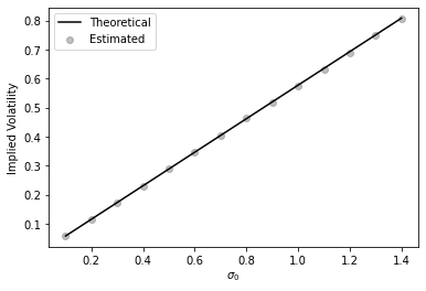
In Figures 1 and 2, we present the results of a Monte Carlo simulation aimed at numerically estimating the skew and the level of the at-the-money implied volatility of the Inverse European call option under the SABR model. We conclude that the numerical results match the theoretical ones.
 |
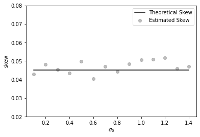 |
| (a) =-0.3 | (b) =0.3 |
5.2 The fractional Bergomi model
The fractional Bergomi stochastic volatility model (see Alòs et al. [4, Chapter 5]) asssumes equation (1) with
where and . For , we have
Then, applying Theorem 1 we obtain that (see Appendix C for the details)
| (19) |
and for
| (20) |
In contrast to the SABR model, the fractional Bergomi model introduces the parameter into the analytical expression for the skew. Note that equation (19) relies on condition . In this case, the ATM implied volatility skew is either zero or depends solely on the product of and . Therefore, the sign of the skew is fully determined by the sign of .
We observe that in the case of rough volatility, i.e., , the skew behaves as , which causes it to diverge. However, as shown in (20), a properly scaled skew takes a finite value, and its sign remains determined by the sign of , with the skew being an increasing function of vol-of-vol. The dependence on is fully non-linear.
The blow-up of the ATM skew limit in the case of rough volatility is the same phenomenon observed in vanilla options, as discussed in [7]. The intuitive explanation is that ATM options are highly uncertain, with a 50/50 chance of becoming in- or out-of-the-money. As the option’s maturity shrinks, this uncertainty increases because there is less time for the price to rebound if it moves in favour of the option. This increases the risk of significant losses if unexpected market changes occur. To hedge against this risk, market makers widen spreads in terms of volatility points, which explains the observed IV skew in real market data. Mathematically, the rough volatility model captures the idea that volatility itself has volatility. Driven by fractional Brownian motion, this model accounts for abrupt shifts in volatility, which are reflected in the adjustment of the IV skew in the Black-Scholes model.
The parameters used for the Monte Carlo simulation are as follows:
and .
To estimate the price of the Inverse European call option under the fractional Bergomi model, we use antithetic variates as presented in equations (17). For the estimation of the skew, we use equation (18).
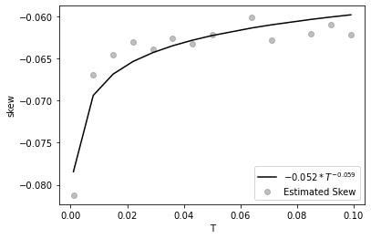
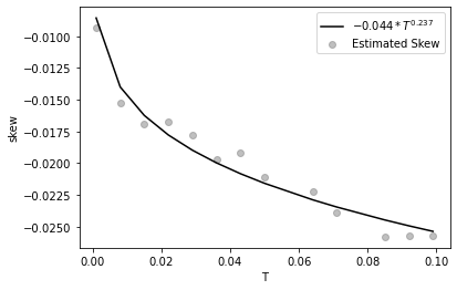
In Figure 3, we present the ATM implied volatility skew as a function of maturity for the Inverse European call option, considering two different values of . We observe the blow-up to for the case . To demonstrate that the fractional Bergomi model captures the power-law structure of the ATM implied volatility skew, we fit the estimated skew to a power-law function , where . Recall that this power-law structure depends on . According to Theorem 1, when , the skew should diverge as , and when , it should approach zero as . However, in Figure 3, we obtain fits of and , respectively. This difference is attributed to the numerical instability of the finite-difference estimation at short maturities in the presence of rough noise. This issue could be improved by significantly increasing the number of Monte Carlo samples or applying a variance reduction technique.
 |
 |
| (a) H=0.4, | (b) H=0.7, |
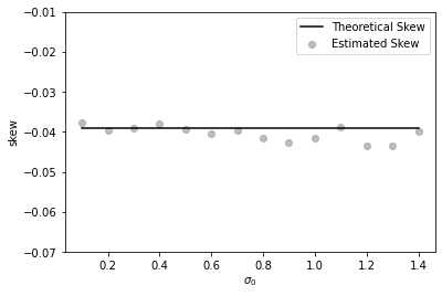
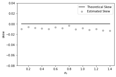
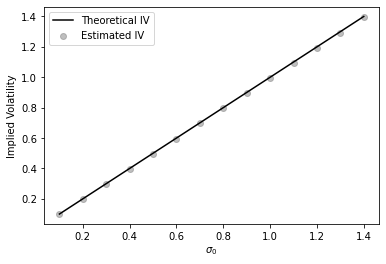
Due to the blow-up of the at-the-money implied volatility skew of the Inverse European call option when , we also plot the quantities for and for in Figure 4. In Figure 5, we present the estimates of the ATM IV level. We conclude that the theoretical results are in line with the values provided by Theorem 1.
 |
 |
| (a) H=0.4 | (b) H=0.7 |
 |
 |
| (a) H=0.4 | (b) H=0.7 |
5.3 Empirical Application
In this section, we demonstrate how the results of Theorem 1 can be applied to empirical data. We consider Bitcoin options traded on Deribit111https://www.deribit.com/options/BTC on 7 May 2024. The spot price is US dollars, and we use 10 different maturities expressed in years, given by the following set of values:
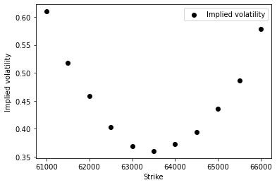
Since our theoretical results are stated as an asymptotic limit, we plot in Figure 6 the implied volatility as a function of the strike for the shortest available maturity, which is 1 day. Recall that the first part of Theorem 1 states . Hence, we conclude that the market estimate of is approximately 0.36.
The second part of Theorem 1 says that
To estimate the implied roughness of the volatility process and identify a class of models that can capture the observed market structure, we begin by estimating the at-the-money implied volatility skew using a standard market approach.
Note that the crypto derivatives market is sufficiently liquid, allowing us to obtain current market quotes for a wide region of the implied volatility surface. In particular, the most liquid part of the market corresponds to delta options, which is exactly the region on which we focus. For a detailed discussion on this topic, see Mixon [24].
More specifically, for each available maturity, we set
Where and represent the market implied volatility of a put and call option with a delta of 0.25, respectively.
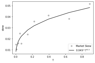
Next, we check whether the power-law structure holds for the at-the-money implied volatility skew as a function of maturity. We fit the function , where , to the estimated ATMIV skew using a standard ordinary least squares (OLS) estimator. The result is presented in Figure 7. We observe that the power-law fits the market at-the-money skew adequately, with , which implies that the market estimation of the Hurst parameter from our data is approximately 0.8.
It is important to note that we are not estimating from the underlying asset’s trajectories but rather from the skew values obtained from the market (see, for instance, Itkin [22]). Furthermore, the market ATMIV skew for the shortest maturity is 0.014, which is consistent with our theoretical formula (19).
Recall that a zero skew means that 0.25 delta calls and puts are priced at the same level of implied volatility, indicating that there is no extra risk premium associated with put options. In contrast to regular markets, where put options are considered insurance against downside movement and are thus in greater demand, leading to elevated implied volatility in comparison to equivalent call options.
We also observe that the SABR model is not suitable for modeling our observed market implied volatility. There are two main reasons for this. First, it is well-known that the SABR implied volatility surface, along with its approximation through Hagan’s formula, cannot accurately reproduce the power-law term structure of the at-the-money skew. Second, formula (16) implies that in order to fit a positive short-end skew, we must force to be positive. However, the assumption that the underlying spot price is positively correlated with volatility contradicts observed data in regular markets and warrants further investigation.
In summary, through Theorem 1, we are able to identify a class of models that can accurately model the market implied volatility surface and draw meaningful conclusions regarding the market’s implied estimates of the corresponding model parameters.
Although the scope of this analysis may seem limited due to the non-monotonicity of implied volatility, this is a common issue in derivatives pricing. For example, calibrating parametric models to the market-implied volatility surface is ill-posed, as the relationship between model parameters and implied volatility is non-unique (e.g., in the SABR, Heston, and fractional Bergomi models). In practice, this non-uniqueness is addressed by selecting the most relevant volatility level for the current market state. Moreover, short-maturity implied volatility often plays a key role in the surface and can serve as a good starting point for approximating the entire curve. While non-uniqueness complicates theoretical analysis, defined values at short maturities often provide reliable approximations for longer maturities.
In terms of trading, short-dated options are actively traded, particularly on platforms like Deribit, which has become a leader in cryptocurrency options. These options, typically expiring daily or weekly, are popular for capitalizing on short-term volatility. Deribit’s trading volume data shows a 99 year-over-year increase in 2024, reflecting the growing demand for options. Traders use short-term options to hedge or exploit event-driven market fluctuations. As a result, there is an increasing need for analytical models for crypto options. The formulas presented here are applicable to options with maturities up to six months, as demonstrated, for example, in Alòs et al.[8].
Disclosure statement
No potential conflict of interest was reported by the authors.
Appendix A A primer on Malliavin Calculus
We introduce the elementary notions of the Malliavin calculus used in this paper (see Nualart and Nualart [25]). Consider a standard Brownian motion defined on a complete probability space and the corresponding filtration generated by . Let be the set of random variables of the form
with , denotes the Wiener integral of the function , for , and (i.e., and all its partial derivatives are bounded). Then the Malliavin derivative of , , is defined as the stochastic process given by
This operator is closable from to , for all , and we denote by the closure of with respect to the norm
We also consider the iterated derivatives for all integers whose domains will be denoted by , for all . We will use the notation .
We denote by the adjoint of the derivative operator and by Dom it domain. If belongs to Dom , then is called the Skorohod integral of , since the set of -adapted processes in is included in Dom , and for such processes the Skorohod integral coincides with the Itô’s integral. We shall use the notation , for any Dom . We recall that is included in the domain of for all and that for all Dom .
One of the main results in Malliavin calculus is the Clark-Ocone-Haussman formula.
Theorem 3.
Let . Then
The following theorem is an extension of classical Ito’s lemma for the case of non-anticipating processes, see Alòs [3] for details.
Theorem 4 (Anticipating Itô’s Formula).
Consider a process of the form
where is a -measurable random variable and and are -adapted processes in .
Consider also a process , for some . Let be a function such that there exists a positive constant such that, for all , and its derivatives evaluated in are bounded by . Then it follows that for all ,
where and the integral is a Skorohod integral since the process is not adapted.
Appendix B The inverse of the ATM Inverse call option price
Recall that ATM value of an Inverse call option is given by
We plot this function in Figure 8 as a function of and observe that the function is not monotonic over its entire domain. As a result, the inverse with respect to will not be uniquely defined. However, since we are primarily interested in the behavior of the function for small values of , in this region the function is monotonically increasing, and the inverse will be well-defined within a small positive interval around zero.
Lemma 2.
Under Hypothesis 1, for all sufficiently small there exists a positive constant such that for all ,
where .
Proof.
We have that
| (21) | ||||
Recall form (13) that
| (22) | ||||
where . Therefore, we conclude that
Notice that , and for sufficiently small , the function is non-negative and monotonically decreasing on the interval . Since is continuous, it is lower bounded by a positive constant on that interval. Additionally, is also small for sufficiently small , ensuring that the inverse is well-defined in this case. This completes the proof. ∎
Lemma 3.
Under Hypothesis 1, for all sufficiently small there exists a positive constant such that for all ,
where .
Proof.
We have that
Therefore,
where . Notice that , and for sufficiently small , the function is non-negative and monotonically increasing on the interval . Since is continuous, it is upper bounded by a positive constant on that interval. Additionally, is small for sufficiently small , ensuring that the inverse is well-defined in this case. This completes the proof. ∎
Lemma 4.
Under Hypothesis 1, for all sufficiently small there exists a positive constant such that for all ,
Appendix C Truncation argument
We present here the truncation argument needed in order to apply Theorem 1 for the SABR and fractional Bergomi models introduced in Sections 5.1 and 5.2.
We start with the SABR model defined in Section 5.1. We define . For every , we consider a function satisfying that for any , for , and for . We set
It is easy to see that satisfies Hypotheses 1, 2, 3, and (2). In fact, for , we have that
which implies that (2) holds with and Hypothesis 2 is satisfied with . Therefore, appealing to Theorem 1 and using the fact that , we conclude that for all ,
| (24) |
where denotes the implied volatility under the volatility process . We then write
| (25) |
By the mean value theorem,
for some , where is the option price under and is defined in Appendix B. Thus, for sufficiently small and , appealing to Lemma 2 we get that
for some constant that changes from line to line. Then, Markov’s inequality implies that for all ,
Thus, taking and using (24) and (25), we conclude that
| (26) |
which shows the validity of (6) for the SABR model.
Next, we prove (16). For , we have
which implies that (3) holds with . Therefore, appealing to Theorem 1 we get that
Since , using dominated convergence theorem, we get that uniformly for all ,
Next, similarly as above we can write
By the mean value theorem,
for some . Then, appealing to Lemma 4 and proceeding exactly as above, we get that for sufficiently large ,
which concludes the proof of (16).
We next prove (26), (19) and (20) for the fractional Bergomi model. We define and as for the SABR model, and we set
It is easy to see that satisfies Hypotheses 1, 2, 3, and (2). In fact, for , we have that
which implies that Hypothesis (2) holds and Hypothesis 2 is satisfied with . Moreover, for , we have
which implies that (3) holds. Therefore, by Theorem 1 we get that (24) holds. We next follow the same computations as the SABR model, but using the fractional Bergomi, to get that for sufficiently small and ,
for some constant . Then, Markov’s inequality implies that for all
Thus, taking , the above shows that for sufficiently large,
which concludes the proof of (26).
Concerning the proof of (19) and (20), on one hand, appealing to Theorem 1, we get that
On the other hand, following along the same lines as above, one can easily show that for sufficiently large
| (27) |
Thus, using dominated convergence we get that uniformly for all ,
Then, computing this integral and using (27), we conclude that (19) and (20) hold true.
References
- [1] Carol Alexander, Ding Chen, and Arben Imeraj. Inverse and Quanto Inverse Options in a Black-Scholes World. Mathematical Finance, 33(4):1005–1043, 2023.
- [2] Carol Alexander and Arben Imeraj. Delta Hedging Bitcoin Options with a Smile. Quantitative Finance, 23(5):799–817, 2023.
- [3] Elisa Alòs. A generalization of the Hull and White formula with applications to option pricing approximation. Finance and Stochastics, 10(3):353–365, 2006.
- [4] Elisa Alòs, David García Lorite, and Dariusz Gatarek. Malliavin Calculus in Finance. Chapman and Hall/CRC Financial Mathematics Series, 2021.
- [5] Elisa Alòs, David García-Lorite, and Aitor Muguruza Gonzalez. On Smile Properties of Volatility Derivatives: Understanding the VIX Skew. SIAM Journal on Financial Mathematics, 13(1):32–69, 2022.
- [6] Elisa Alòs and Jorge A. León. On the curvature of the smile in stochastic volatility models. SIAM Journal on Financial Mathematics, 8:373–399, 2017.
- [7] Elisa Alòs, Jorge A. León, and Josep Vives. On the short-time behavior of the implied volatility for jump-diffusion models with stochastic volatility. Finance and Stochastics, 11(4):571–589, 2007.
- [8] Elisa Alòs, Eulalia Nualart, and Makar Pravosud. On the implied volatility of Asian options under stochastic volatility models. Applied Mathematical Finance, pages 1–26, 2024.
- [9] Elisa Alòs and Kenichiro Shiraya. Estimating the Hurst parameter from short term volatility swaps: a Malliavin calculus approach. Finance and Stochastics, 23(2):423–447, 2019.
- [10] Saifedean Ammous. Can cryptocurrencies fulfil the functions of money? The Quarterly Review of Economics and Finance, 70:38–51, 2018.
- [11] Thomas Ankenbrand and Denis Bieri. Assessment of cryptocurrencies as an asset class by their characteristics. Investment Management and Financial Innovations, 15(3):169–181, 2018.
- [12] Olyga S. Bolotaeva, Amalia A. Stepanova, and Sofia S. Alekseeva. The Legal Nature of Cryptocurrency. IOP Conference Series: Earth and Environmental Science, 272(3):032166, 2019.
- [13] Fabienne Comte and Eric Renault. Long memory in continuous-time stochastic volatility models. Mathematical finance, 8(4):291–323, 1998.
- [14] Rama Cont and Purba Das. Rough Volatility: Fact or Artefact? Sankhya B, 86:191–323, 2024.
- [15] Anne Haubo Dyhrberg. Bitcoin, gold and the dollar – A GARCH volatility analysis. Finance Research Letters, 16:85–92, 2016.
- [16] Mark B. Garman and Steven W. Kohlhagen. Foreign currency option values. Journal of International Money and Finance, 2(3):231–237, 1983.
- [17] Stéphane Goutte, Khaled Guesmi, and Samir Saadi. Cryptofinance. WORLD SCIENTIFIC, 2021.
- [18] Marc Gronwald. Is Bitcoin a Commodity? On price jumps, demand shocks, and certainty of supply. Journal of International Money and Finance, 97:86–92, 2019.
- [19] Patrik Hagan, Andrew Lesniewski, and Diana Woodward. Managing smile risk. Wilmott Magazine, 1:84–102, 2002.
- [20] Peter K. Hazlett and William J. Luther. Is bitcoin money? And what that means. The Quarterly Review of Economics and Finance, 77:144–149, 2020.
- [21] Ai Jun Hou, Weining Wang, Cathy Y. H. Chen, and Wolfgang Karl Härdle. Pricing Cryptocurrency Options. Journal of Financial Econometrics, 18(2):250–279, 2020.
- [22] Andrey Itkin. Short time behavior of the ATM implied skew in the ADO-Heston model. Frontiers of Mathematical Finance, 3(2):214–238, 2024.
- [23] Jovanka Lili Matic, Natalie Packham, and Wolfgang Karl Härdle. Hedging cryptocurrency options. Review of Derivatives Research, 26(1):91–133, 2023.
- [24] Scott Mixon. What Does Implied Volatility Skew Measure? The Journal of Derivatives, 18(4):9–25, 2011.
- [25] David Nualart and Eulalia Nualart. Introduction to Malliavin Calculus. Cambridge University Press, 2018.
- [26] Dan Pirjol and Lingjiong Zhu. Short maturity Asian options in local volatility models. SIAM Journal on Financial Mathematics, 7:947–992, 2016.
- [27] Tak Kuen Siu and Robert J. Elliott. Bitcoin option pricing with a SETAR-GARCH model. The European Journal of Finance, 27(6):564–595, 2021.