On the Interplay between Sparsity, Naturalness,
Intelligibility, and Prosody in Speech Synthesis
Abstract
Are end-to-end text-to-speech (TTS) models over-parametrized? To what extent can these models be pruned, and what happens to their synthesis capabilities? This work serves as a starting point to explore pruning both spectrogram prediction networks and vocoders. We thoroughly investigate the tradeoffs between sparsity and its subsequent effects on synthetic speech. Additionally, we explore several aspects of TTS pruning: amount of finetuning data versus sparsity, TTS-Augmentation to utilize unspoken text, and combining knowledge distillation and pruning. Our findings suggest that not only are end-to-end TTS models highly prunable, but also, perhaps surprisingly, pruned TTS models can produce synthetic speech with equal or higher naturalness and intelligibility, with similar prosody. All of our experiments are conducted on publicly available models, and findings in this work are backed by large-scale subjective tests and objective measures. Code and 200 pruned models are made available to facilitate future research on efficiency in TTS111Project webpage: https://people.csail.mit.edu/clai24/prune-tts/.
Index Terms— text-to-speech, vocoder, speech synthesis, pruning, efficiency
1 Introduction
End-to-end text-to-speech (TTS)222We refer to end-to-end TTS systems as those composed of an acoustic model (also known as text-to-spectrogram prediction network) and a separate vocoder, as there are relatively few direct text-to-waveform models; see [1]. research has focused heavily on modeling techniques and architectures, aiming to produce more natural, adaptive, and expressive speech in robust, low-resource, controllable, or online conditions [1]. We argue that an overlooked orthogonal research direction in end-to-end TTS is architectural efficiency, and in particular, there has not been any established study on pruning end-to-end TTS in a principled manner. As the body of TTS research moves toward the mature end of the spectrum, we expect a myriad of effort delving into developing efficient TTS, with direct implications such as on-device TTS or a better rudimentary understanding of training TTS models from scratch [2].
To this end, we provide analyses on the effects of pruning end-to-end TTS, utilizing basic unstructured magnitude-based weight pruning333Given that there has not been a dedicated TTS pruning study in the past, we resort to the most basic form of pruning. For more advanced pruning techniques, please refer to [3, 4].. The overarching message we aim to deliver is two-fold:
-
•
End-to-end TTS models are over-parameterized; their weights can be pruned with unstructured magnitude-based methods.
-
•
Pruned models can produce synthetic speech at equal or even better naturalness and intelligibility with similar prosody.
To introduce our work, we first review two areas of related work: Efficiency in TTS One line of work is on small-footpoint, fast, and parallelizable versions of WaveNet [5] and WaveGlow [6] vocoders; prominent examples are WaveRNN444Structured pruning was in fact employed in WaveRNN, but merely for reducing memory overhead for the vocoder. What sets this work apart is our pursuit of the scientific aspects of pruning end-to-end TTS holistically. [7], WaveFlow [8], Clarinet [9], HiFi-GAN [10], Parallel WaveNet [11], SqueezeWave [12], DiffWave [13], WaveGrad 1 [14], Parallel WaveGAN [15] etc. Another is acoustic models based on non-autoregressive generation (ParaNet [16], Flow-TTS [17], MelGAN [18], EfficientTTS [19], FastSpeech [20, 21]), neural architecture search (LightSpeech [22]), diffusion (WaveGrad 2 [23]), etc. Noticeably, efficient music generation has gathered attention too, e.g. NEWT [24] and DDSP [25].
ASR Pruning Earlier work on ASR pruning reduces the FST search space, such as [26]. More recently, the focus has shifted to pruning end-to-end ASR models [27, 28, 29, 30]. Generally speaking, pruning techniques proposed for vision models [3, 4] work decently well in prior ASR pruning work, which leads us to ask, how effective are simple pruning techniques for TTS?
This work thus builds upon a recent ASR pruning technique termed [30], with the intention of not only reducing architectural complexity for end-to-end TTS, but also demonstrating the surprising efficacy and simplicity of pruning in contrast to prior TTS efficiency work. We first review in Section 2. In Section 3, we describe our experimental and listening test setups, and in Section 4 we present results with several visualizations. Our contributions are:
- •
-
•
We extend with knowledge distillation () and TTS-Augmentation [33] for TTS pruning, demonstrating ’s applicability and effectiveness regardless of network architectures or input/output pairs.
-
•
We show that end-to-end TTS models are over-parameterized. Pruned models produce speech with similar levels of naturalness, intelligibility, and prosody to that of unpruned models.
-
•
For instance, with large-scale subjective tests and objective measures, Transformer-TTS at 30% sparsity has statistically better naturalness than its original version; for another, small footprint CNN-based vocoder has little to no synthesis degradation at up to 88 sparsity.
2 Method
2.1 Problem Formulation
Consider a sequence-to-sequence learning problem, where and represent the input and output sequences respectively. For ASR, is waveforms and is character/phone sequences; for a TTS acoustic model, is character/phone sequences and is spectrogram sequences; for a vocoder, is spectrogram sequences and is waveforms. A mapping function parametrized by a neural network is learned, where represents the network parameters and represents the number of parameters. Sequence-level log-likelihood on target dataset is maximized.
Our goal is to find a subnetwork , where is the element-wise product and a binary pruning mask is applied on the model weights . The ideal pruning method would learn at target sparsity such that achieves similar loss as after training on .
2.2 Pruning Sequence-to-Sequence Models with
Unstructured Magnitude Pruning () [2, 3] sorts the model’s weights according to their magnitudes across layers regardless of the network structure, and removes the smallest ones to meet a predefined sparsity level. Weights that are pruned out (specified by ) are zeroed out and do not receive gradient updates during training.
Iterative Magnitude Pruning () [2, 3] is based on and assumes an initial model weight and a target dataset are given. can be described as:
-
1.
Directly prune at target sparsity, and obtain an initial pruning mask . Zero out weights in given by .
-
2.
Train on until convergence. Zeroed-out weights do not receive gradient updates via backpropogation.
The above procedure can be iterated multiple times by updating with the finetuned model weight from Step 2.
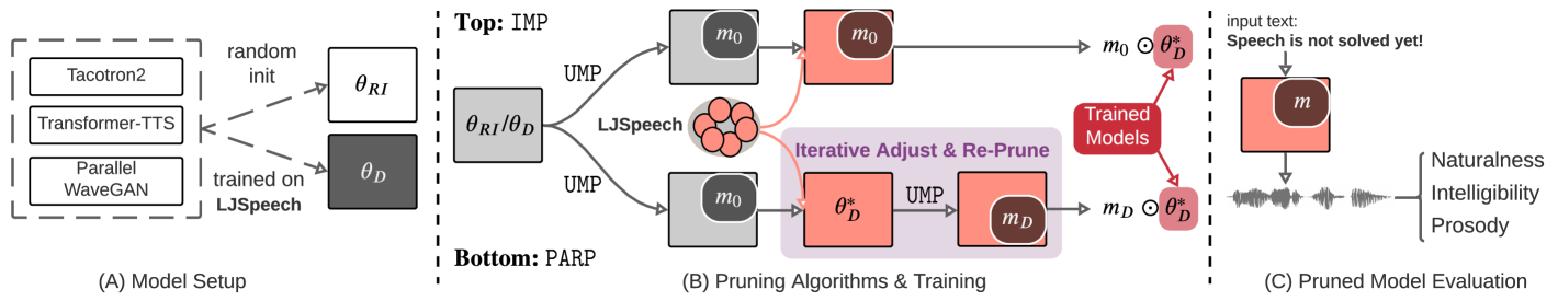
Prune-Adjust-Re-Prune () [30] is a simple modified version of recently proposed for self-supervised speech recognition, showing that pruned wav2vec 2.0 [34] attains lower WERs than the full model under low-resource conditions. Given its simplicity, here we show that can be applied to any sequence-to-sequence learning scenario. Similarly, given an initial model weight and , can be described as (See Fig 1 for visualization):
-
1.
Same as ’s Step 1.
-
2.
Train on . Zeroed-out weights in receive gradient updates via backprop. After model updates, obtain the trained model , and apply on to obtain mask . Return subnetwork .
Setting Initial Model Weight In [30], ’s can be the self-supervised pretrained initializations, or any trained model weight ( needs not be the target task ). On the other hand, ’s is target-task dependent i.e. is set to a trained weight on , denoted as . However, since the focus in this work is on the final pruning performance only, we set to by default for both and .
Progressive Pruning with - Following [30], we also experiment with progressive pruning (-), where -’s Step 1 prunes at a lower sparsity, and its Step 2 progressively prunes to the target sparsity every model updates. We show later that - is especially effective in higher sparsity regions.
3 Experimental Setup
3.1 TTS Models and Data
Model Configs Our end-to-end TTS is based on an acoustic model (phone to melspec) and a vocoder (melspec to wav). To ensure reproducibility, we used publicly available and widely adopted implementations555Checkpoints are also available at ESPnet and ParallelWaveGAN.: Transformer-TTS [31] and Tacotron2 [32] as the acoustic models, and Parallel WaveGAN [15] as the vocoder. Transformer-TTS and Tacotron2 have the same high-level structure (encoder, decoder, pre-net, post-net) and loss (l2 reconstructions before and after post-nets and stop token cross-entropy). Transformer-TTS consists of a 6-layer encoder and a 6-layer decoder. Tacotron2’s encoder consists of 3-layer convolutions and a BLSTM, and its decoder is a 2-layer LSTM with attention. Both use a standard G2P for converting text to phone sequences as the model input. Parallel WaveGAN consists of convolution-based generator and discriminator .
Datasets LJspeech [35] is used for training acoustic models and vocoders. It is a female single-speaker read speech corpus with 13k text-audio pairs, totaling 24h of recordings. We also used the transcription of Librispeech’s train-clean-100 partition [36] as additional unspoken text666Both LJspeech and Librispeech are based on audiobooks. used in TTS-Augmentation.
3.2 Implementation
is based on PyTorch’s API777PyTorch Pruning API. For all models, is set to pretrained checkpoints on LJspeech, and is set to 1 epoch of model updates. We jointly prune encoder, decoder, pre-nets, and post-nets for the acoustic model; for vocoder, since only is needed during test-time synthesis, only is pruned ( is still trainable).
3.3 Complementary Techniques for
TTS-Augmentation for unspoken transcriptions The first technique is based on TTS-Augmentation [33]. It is a form of self-training, where we take to label additional unspoken text . The newly synthesized paired data, denoted , is used together with in ’s Step 2.
Combining Knowledge-Distillation () and , with a teacher model denoted as . The training objective in ’s Step 2 is set to reconstructing both ground truth melspec and melspec synthesized by an (unpruned) teacher acoustic model .
3.4 Subjective and Objective Evaluations
We examine the following three aspects of the synthetic speech:
-
•
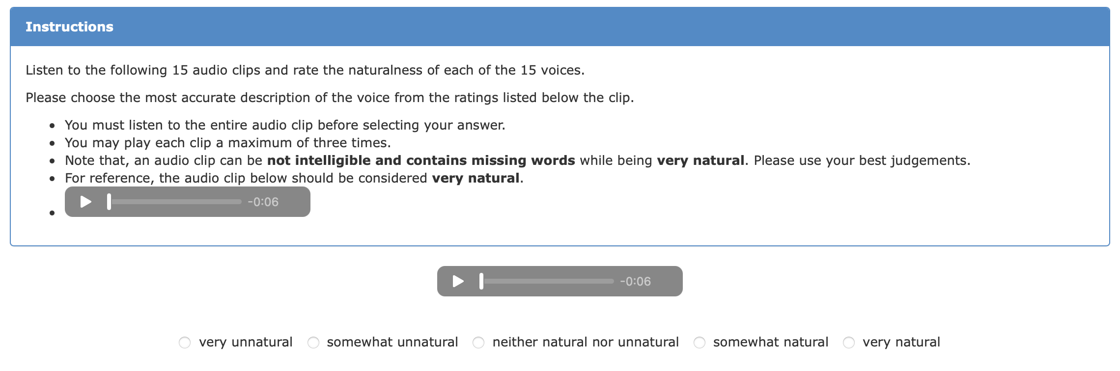
Naturalness is quantified by the 5-point (1-point increment) scale Mean Opinion Score (MOS). 20 unique utterances (with 5 repetitions) are synthesized and compared across pruned models, for a total of 100 HITs (crowdsourced tasks) per MOS test. In each HIT, the input texts to all models are the same to minimize variability.
-
•
Intelligibility is measured with Google’s ASR API888https://pypi.org/project/SpeechRecognition/.
-
•
Prosody via mean and standard deviation (std) fundamental frequency () estimations999 estimation with probabilistic YIN (pYIN) implemented in Librosa. and utterance duration, averaged over dev and eval utterances.
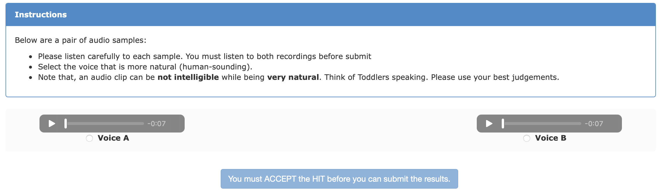
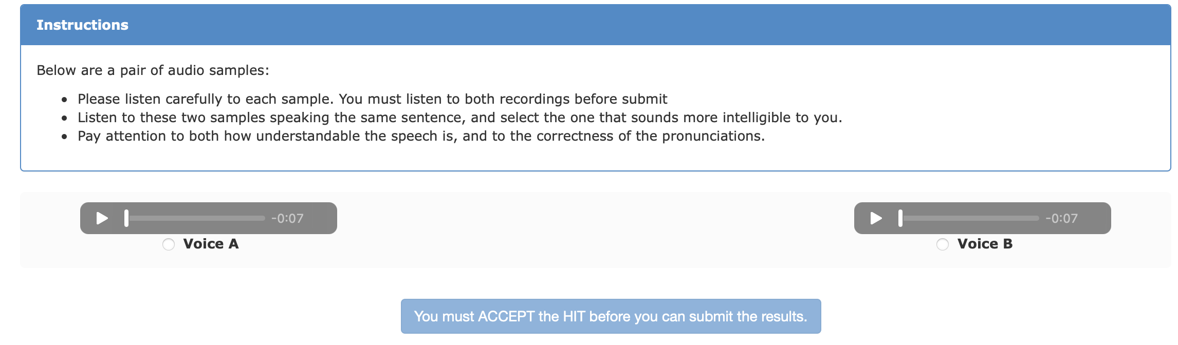
We also perform pairwise comparison (A/B) testings for naturalness and intelligibility (separately). Similar to our MOS test, we release 20 unique utterances (with 10 repetitions), for a total of 200 HITs per A/B test. In each HIT, input text to models are also the same. MOS and A/B tests are conducted in Amazon Mechanical Turk (AMT).
Statistical Testing To ensure our AMT results are statistically significant, we run Mann-Whitney U test for each MOS test, and pairwise z-test for each A/B test, both at significance level of .
4 Results
4.1 Does Sparsity improve Naturalness?
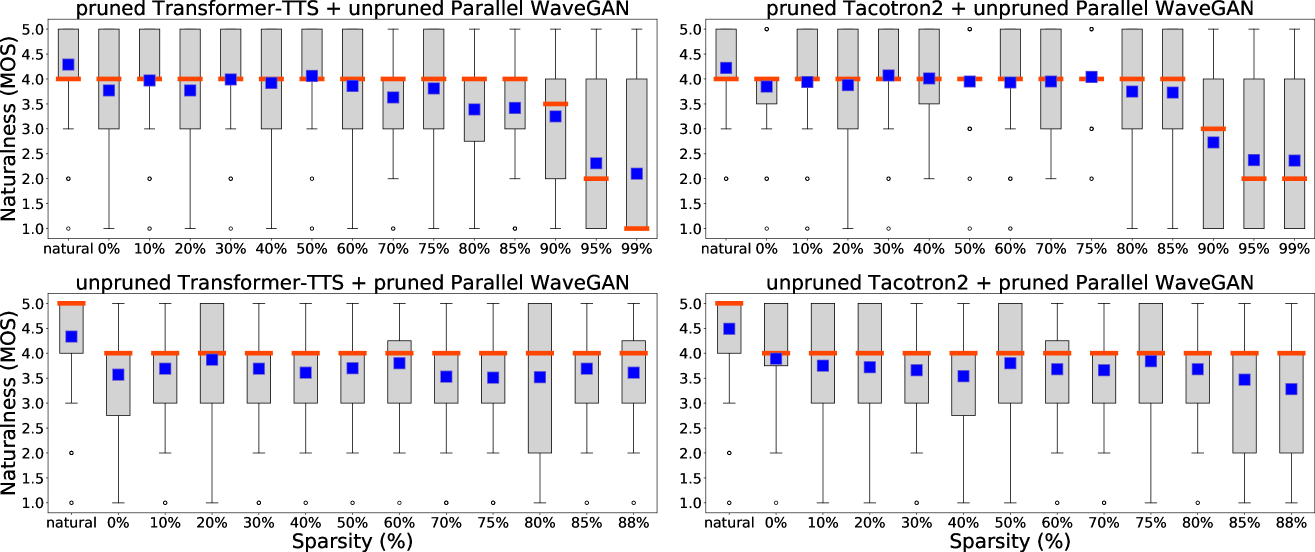
Fig 2 is the box plot of MOS scores of pruned end-to-end TTS models at 0%99% sparsities with . In each set of experiments, only one of the acoustic model or vocoder is pruned, while the other is kept intact. For either pruned Transformer-TTS or Tacotron2 acoustic models, their MOS scores are statistically not different from the unpruned ones at up to 90% sparsity. For pruned Parallel WaveGAN, pairing it with an unpruned Transformer-TTS reaches up to 88% sparsity without any statistical MOS decrease, and up to 85% if paired with an unpruned Tacotron2. Based on these results, we first conclude that end-to-end TTS models are over-parameterized across model architectures, and removing the majority of their weights does not significantly affect naturalness.
Secondly, we observe that the 30% pruned Tacotron2 has a statistically higher MOS score than unpruned Tacotron2. Although this phenomenon is not seen in Transformer-TTS, WaveGAN, or at other sparsities, it is nonetheless surprising given ’s simplicity. We can hypothesize that under the right conditions, pruned models train better, which results in higher naturalness over unpruned models.
4.2 Does Sparsity improve Intelligibility?
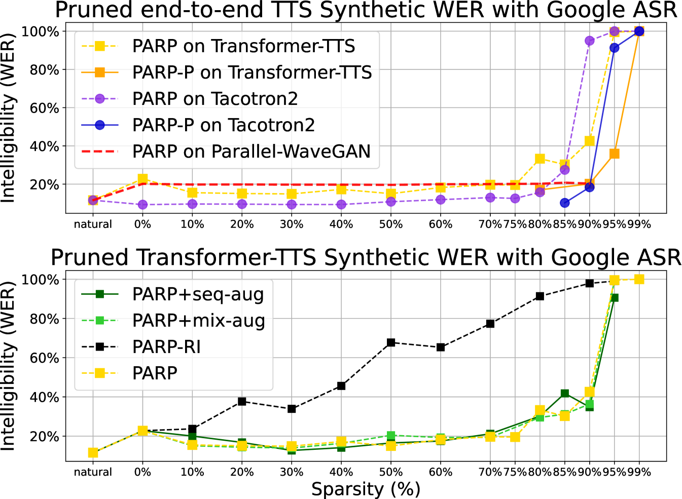
We measure intelligibility of synthetic speech via Google ASR, and Figure 3 plots synthetic speech’s WERs across sparsities over model and pruning configurations. Focusing on the top plot, we have the following two high-level impressions: (1) WER decreases at initial sparsities and increases dramatically at around 85% sparsity with (yellow and purple dotted lines). (2) pruning the vocoder does not change the WERs at all (observe the straight red dotted line).
Specifically, for Transformer-TTS, at 75% and - at 90% sparsities have lower WERs (higher intelligibility) than its unpruned version. For Tacotron2, there is no WER reduction and its WERs remain at 9% at up to 40% sparsity (no change in intelligibility). Based on (2) and Section 4.1, we can further conclude that the CNN-based vocoder is highly prunable, with little to no naturalness and intelligibility degradation at up to almost 90% sparsity.
4.3 Does Sparsity change Prosody?
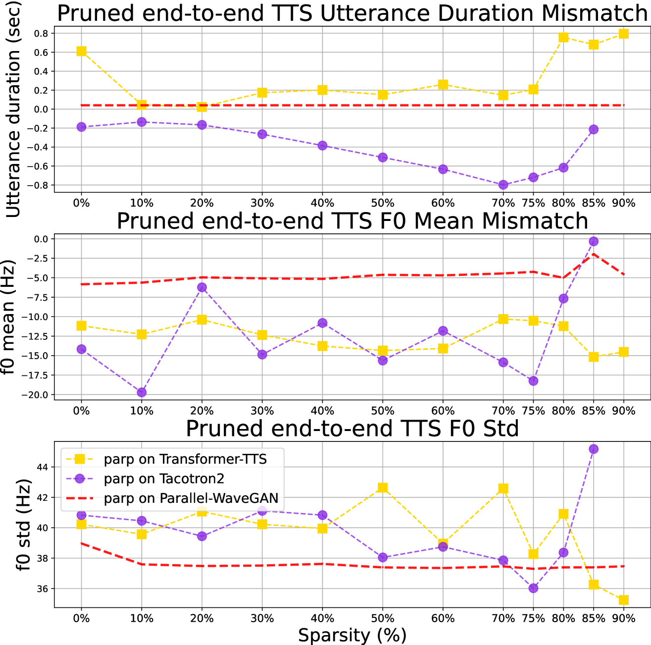
We used synthetic speech’s utterance duration and mean/std across time as three rough proxies for prosody. Fig 4 plots the prosody mismatch between pruned models and ground truth recordings across model combinations. Observe on Tacotron2 and on Transformer-TTS result in visible differences in prosody changes over sparsities. In the top plot, pruned Transformer-TTS (yellow dotted line) have the same utterance duration (+0.2 seconds over ground truth) at 10%75% sparsities, while in the same region, pruned Tacotron2 (purple dotted line) results in a linear decrease in duration (-0.2-0.8 seconds). Indeed, we confirmed by listening to synthesis samples that pruning Tacotron2 leads to shorter utterance duration as sparsity increases.
In the middle plot and up to 80% sparsity, pruned Tacotron2 models have a much large mean variation (-20-7.5 Hz) compared to that of Transformer-TTS (-10-15 Hz). We hypothesize that on RNN-based models leads to unstable gradients through time during training, while Transformer-based models are easier to prune. Further, on WaveGAN (red dotted line) has a minimal effect on both metrics across sparsities, which leads us to another hypothesis that vocoder is not responsible for prosody generation.
4.4 Does more finetuning data improve sparsity?
In [30], the authors attain pruned wav2vec 2.0 at much higher sparsity without WER increase given sufficient finetuning data (10h Librispeech split). Therefore, one question we had was, how much finetuning data is “good enough” for pruning end-to-end TTS? We did two sets of experiments, and for each, we modify the amount of data in ’s Step 2, while keeping as is (trained on full LJspeech).
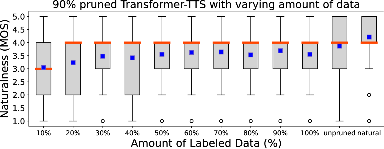
The first set of experiments result is Fig 5. Even at as high as 90% sparsity, 30% of finetuning data (7.2h) is enough for to reach the same level of naturalness as full data101010The effect of using less data to obtain remains unclear.. The other set of experiment is TTS-Augmentation for utilizing additional unspoken text (100h, no domain mismatch) for ’s Step 2. In Fig 3’s bottom plot, we see TTS-Augmentations (dark & light green lines) bear minimal effect on the synthetic speech WERs. However, Table 1 indicates that TTS-Augmentation +- does statistically improve in naturalness and intelligibility subjective testings.
4.5 Ablations
Knowledge Distillation hurts Surprisingly, we found combining knowledge distillation from teacher model with significantly reduces the synthesis quality, see + v.s. in Table 1. Perhaps more careful tuning is required to make work.
Importance of Bottom plot of Fig 3 (black dotted line) and Table 1 ( v.s. -) demonstrate the importance of setting the initial model weight . In both cases, we set to random initialization () instead of on LJspeech.
Effectiveness of Table 1 shows the clear advantage of - over at high sparsities, yet is not strictly better than .
| Proposal | Baseline | Sparsity | Preference over Baseline | |
| Level | Naturalness | Intelligibility | ||
| pruned Transformer-TTS + unpruned Parallel WaveGAN | ||||
| - | 90% | 57% | 66% | |
| 95% | 63% | 64% | ||
| + | 70% | 40% | 43% | |
| 90% | 36% | 27% | ||
| - | 90% | 53% | 51% | |
| 95% | 64% | 61% | ||
| 30% | 54% | 58% | ||
| 50% | 46% | 54% | ||
| 90% | 42% | 37% | ||
| - | 10% | 55% | 57% | |
| 30% | 55% | 53% | ||
| 50% | 56% | 67% | ||
| 70% | 53% | 53% | ||
| 90% | 60% | 56% | ||
| +- | 10% | 58% | 58% | |
| 30% | 52% | 57% | ||
| 50% | 44% | 41% | ||
| 70% | 57% | 54% | ||
| 90% | 51% | 56% | ||
5 Remarks
Significance This work is scientific in nature, as most of our results arose from analyzing pruned models via large-scale experimentation and testing. In fact, we are less interested in answering questions like “how much can Tacotron2 be reduced to?”, and more curious about inquiries along the line of, “what are patterns/properties unique to end-to-end TTS?” Continuing in this direction should allow us to understand more in depth how end-to-end TTS models are trained.
Future Work Possible extensions upon this work are 1) inclusion of an ASR loss term in PARP’s step 2 for melspec pruning, 2) multi-lingual/multi-speaker TTS pruning, 3) further study on why over-parameterization benefit end-to-end TTS, 4) showing the Lottery Ticket Hypothesis [2] exists in end-to-end TTS, and 5) determining if insights from pruning help design better TTS model architectures.
References
- [1] Xu Tan, Tao Qin, Frank Soong, and Tie-Yan Liu, “A survey on neural speech synthesis,” arXiv preprint arXiv:2106.15561, 2021.
- [2] Jonathan Frankle and Michael Carbin, “The lottery ticket hypothesis: Finding sparse, trainable neural networks,” ICLR, 2019.
- [3] Trevor Gale, Erich Elsen, and Sara Hooker, “The state of sparsity in deep neural networks,” arXiv preprint arXiv:1902.09574, 2019.
- [4] Davis Blalock, Jose Javier Gonzalez Ortiz, Jonathan Frankle, and John Guttag, “What is the state of neural network pruning?,” Conference on Machine Learning and Systems, 2020.
- [5] Aaron van den Oord, Sander Dieleman, Heiga Zen, Karen Simonyan, Oriol Vinyals, Alex Graves, Nal Kalchbrenner, Andrew Senior, and Koray Kavukcuoglu, “Wavenet: A generative model for raw audio,” arXiv preprint arXiv:1609.03499, 2016.
- [6] Ryan Prenger, Rafael Valle, and Bryan Catanzaro, “Waveglow: A flow-based generative network for speech synthesis,” in ICASSP, 2019.
- [7] Nal Kalchbrenner, Erich Elsen, Karen Simonyan, Seb Noury, Norman Casagrande, Edward Lockhart, Florian Stimberg, Aaron Oord, Sander Dieleman, and Koray Kavukcuoglu, “Efficient neural audio synthesis,” in ICML, 2018.
- [8] Wei Ping, Kainan Peng, Kexin Zhao, and Zhao Song, “Waveflow: A compact flow-based model for raw audio,” in ICML, 2020.
- [9] Wei Ping, Kainan Peng, and Jitong Chen, “Clarinet: Parallel wave generation in end-to-end text-to-speech,” ICLR, 2019.
- [10] Jungil Kong, Jaehyeon Kim, and Jaekyoung Bae, “Hifi-gan: Generative adversarial networks for efficient and high fidelity speech synthesis,” NeurIPS, 2020.
- [11] Aaron Oord, Yazhe Li, Igor Babuschkin, Karen Simonyan, Oriol Vinyals, Koray Kavukcuoglu, George Driessche, Edward Lockhart, Luis Cobo, Florian Stimberg, et al., “Parallel wavenet: Fast high-fidelity speech synthesis,” in ICML, 2018.
- [12] Bohan Zhai, Tianren Gao, Flora Xue, Daniel Rothchild, Bichen Wu, Joseph E Gonzalez, and Kurt Keutzer, “Squeezewave: Extremely lightweight vocoders for on-device speech synthesis,” arXiv preprint arXiv:2001.05685, 2020.
- [13] Zhifeng Kong, Wei Ping, Jiaji Huang, Kexin Zhao, and Bryan Catanzaro, “Diffwave: A versatile diffusion model for audio synthesis,” ICLR, 2021.
- [14] Nanxin Chen, Yu Zhang, Heiga Zen, Ron J Weiss, Mohammad Norouzi, and William Chan, “Wavegrad: Estimating gradients for waveform generation,” ICLR, 2021.
- [15] Ryuichi Yamamoto, Eunwoo Song, and Jae-Min Kim, “Parallel wavegan: A fast waveform generation model based on generative adversarial networks with multi-resolution spectrogram,” in ICASSP, 2020.
- [16] Kainan Peng, Wei Ping, Zhao Song, and Kexin Zhao, “Non-autoregressive neural text-to-speech,” in ICML, 2020.
- [17] Chenfeng Miao, Shuang Liang, Minchuan Chen, Jun Ma, Shaojun Wang, and Jing Xiao, “Flow-tts: A non-autoregressive network for text to speech based on flow,” in ICASSP, 2020.
- [18] Kundan Kumar, Rithesh Kumar, Thibault de Boissiere, Lucas Gestin, Wei Zhen Teoh, Jose Sotelo, Alexandre de Brébisson, Yoshua Bengio, and Aaron Courville, “Melgan: Generative adversarial networks for conditional waveform synthesis,” NeurIPS, 2019.
- [19] Chenfeng Miao, Liang Shuang, Zhengchen Liu, Chen Minchuan, Jun Ma, Shaojun Wang, and Jing Xiao, “Efficienttts: An efficient and high-quality text-to-speech architecture,” in ICML, 2021.
- [20] Yi Ren, Yangjun Ruan, Xu Tan, Tao Qin, Sheng Zhao, Zhou Zhao, and Tie-Yan Liu, “Fastspeech: Fast, robust and controllable text to speech,” NeurIPS, 2019.
- [21] Yi Ren, Chenxu Hu, Xu Tan, Tao Qin, Sheng Zhao, Zhou Zhao, and Tie-Yan Liu, “Fastspeech 2: Fast and high-quality end-to-end text to speech,” ICLR, 2021.
- [22] Renqian Luo, Xu Tan, Rui Wang, Tao Qin, Jinzhu Li, Sheng Zhao, Enhong Chen, and Tie-Yan Liu, “Lightspeech: Lightweight and fast text to speech with neural architecture search,” in ICASSP, 2021.
- [23] Nanxin Chen, Yu Zhang, Heiga Zen, Ron J Weiss, Mohammad Norouzi, Najim Dehak, and William Chan, “Wavegrad 2: Iterative refinement for text-to-speech synthesis,” Interspeech, 2021.
- [24] Ben Hayes, Charalampos Saitis, and György Fazekas, “Neural waveshaping synthesis,” ISMIR, 2021.
- [25] Jesse Engel, Lamtharn Hantrakul, Chenjie Gu, and Adam Roberts, “Ddsp: Differentiable digital signal processing,” ICLR, 2020.
- [26] Hainan Xu, Tongfei Chen, Dongji Gao, Yiming Wang, Ke Li, Nagendra Goel, Yishay Carmiel, Daniel Povey, and Sanjeev Khudanpur, “A pruned rnnlm lattice-rescoring algorithm for automatic speech recognition,” in ICASSP, 2018.
- [27] Dong Yu, Frank Seide, Gang Li, and Li Deng, “Exploiting sparseness in deep neural networks for large vocabulary speech recognition,” in ICASSP, 2012.
- [28] Yuan Shangguan, Jian Li, Qiao Liang, Raziel Alvarez, and Ian McGraw, “Optimizing speech recognition for the edge,” arXiv preprint arXiv:1909.12408, 2019.
- [29] Zhaofeng Wu, Ding Zhao, Qiao Liang, Jiahui Yu, Anmol Gulati, and Ruoming Pang, “Dynamic sparsity neural networks for automatic speech recognition,” in ICASSP, 2021.
- [30] Cheng-I Jeff Lai, Yang Zhang, Alexander H Liu, Shiyu Chang, Yi-Lun Liao, Yung-Sung Chuang, Kaizhi Qian, Sameer Khurana, David Cox, and James Glass, “Parp: Prune, adjust and re-prune for self-supervised speech recognition,” NeurIPS, 2021.
- [31] Naihan Li, Shujie Liu, Yanqing Liu, Sheng Zhao, and Ming Liu, “Neural speech synthesis with transformer network,” in AAAI, 2019.
- [32] Jonathan Shen, Ruoming Pang, Ron J Weiss, Mike Schuster, Navdeep Jaitly, Zongheng Yang, Zhifeng Chen, Yu Zhang, Yuxuan Wang, Rj Skerrv-Ryan, et al., “Natural tts synthesis by conditioning wavenet on mel spectrogram predictions,” in ICASSP, 2018.
- [33] Min-Jae Hwang, Ryuichi Yamamoto, Eunwoo Song, and Jae-Min Kim, “Tts-by-tts: Tts-driven data augmentation for fast and high-quality speech synthesis,” in ICASSP, 2021.
- [34] Alexei Baevski, Henry Zhou, Abdelrahman Mohamed, and Michael Auli, “wav2vec 2.0: A framework for self-supervised learning of speech representations,” NeurIPS, 2020.
- [35] Keith Ito and Linda Johnson, “The lj speech dataset,” https://keithito.com/LJ-Speech-Dataset/, 2017.
- [36] Vassil Panayotov, Guoguo Chen, Daniel Povey, and Sanjeev Khudanpur, “Librispeech: an asr corpus based on public domain audio books,” in ICASSP, 2015.
- [37] Heiga Zen, Keiichi Tokuda, and Alan W Black, “Statistical parametric speech synthesis,” speech communication, 2009.
6 Supplementary Materials
6.1 Philosophy
We clarify here again the philosophy of this piece of work – we are interested in quantifying the effects of sparsity on speech perceptions (measured via naturalness, intelligibility, and prosody), as there has not been any systematic study in this direction. The pruning methods, either or , are merely engineering “tools” to probe the underlying phenomenon. It is not too difficult to get higher sparsities or introduce fancier pruning techniques as noted in this study, yet they are less scientifically interesting at this moment.
6.2 Implementation
Normally, s are iterated many times depending on the training costs. In iteration , the mask from the previous iteration is fixed, and only the remaining weights are considered in . In other words, each iteration’s sparsity pattern is built on top of the that from the previous iteration. For simplicity, our implementation only has 1 iteration. In some literature, this is termed One-Shot Magnitude Pruning , though it is also not exactly our case due to our starting point is a fully trained model instead of a randomly initialized model.
6.3 TTS-Augmentation Implementations
We experimented with two TTS-Augmentation policies for with initial model trained on LJspeech and additional unspoken text from Librispeech :
-
•
+-: synthesize with to obtain . First, perform ’s Step 2 at target sparsity on with initial model weight . Obtain a pruned model with model weight . Next, perform ’s Step 2 at target sparsity on with initial model weight . Return .
-
•
+-: synthesize with to obtain . Directly perform ’s Step 2 on with initial model weight . Return .
Table 2 is the subjective A/B testing results comparing the two augmentation policies at different sparsities. Although there is no statistical preference between the two, we note that pruned models with different augmentation policies do subjectively sound different from one another.
| Proposal | Baseline | Sparsity | Preference over Baseline | |
| Level | Naturalness | Intelligibility | ||
| pruned Transformer-TTS + unpruned Parallel WaveGAN | ||||
| +- | +- | 10% | 53% | - |
| 30% | 55% | - | ||
| 50% | 46% | - | ||
| 70% | 47% | - | ||
| 90% | 53% | - | ||
6.4 Statistical Testing Result
Below are the results of running Mann-Whitney U test on our Naturalness MOS tests at a significance level , where indicates pair-wise statistically significant, and indicates the opposite. The order in and axes are shuffled due to our MOS test implementation. Cross reference with Figure 2, we have the following conclusions:
-
•
on Transformer-TTS + unpruned Parallel WaveGAN (Table 3): no pruned model is statistically better than the unpruned model, and pruned model is only statistically worse starting at 90% sparsity.
-
•
on Tacotron2 + unpruned Parallel WaveGAN (Table 4): 30% pruned model is statistically better than the unpruned model, and pruned model is only statistically worse starting at 90% sparsity.
-
•
Unpruned Transformer-TTS + on Parallel WaveGAN (Table 5): no pruned model is statistically better than the unpruned model, and no pruned model model is statistically worse either.
-
•
Unpruned Tacotron2 + on Parallel WaveGAN (Table 6): no pruned model is statistically better than the unpruned model, and pruned model is only statistically worse starting at 85% sparsity.
Based on the above statistical testings, we are not claiming that pruning definitely improves TTS training. Instead, at the right conditions, pruned models could perform better than the unpruned ones.
| natural | 70% | 30% | natural | 99% | 90% | 50% | 95% | full | 80% | 75% | 40% | 85% | 10% | 20% | 60% | |
| natural | - | |||||||||||||||
| 70% | - | |||||||||||||||
| 30% | - | |||||||||||||||
| natural | - | |||||||||||||||
| 99% | - | |||||||||||||||
| 90% | - | |||||||||||||||
| 50% | - | |||||||||||||||
| 95% | - | |||||||||||||||
| full | - | |||||||||||||||
| 80% | - | |||||||||||||||
| 75% | - | |||||||||||||||
| 40% | - | |||||||||||||||
| 85% | - | |||||||||||||||
| 10% | - | |||||||||||||||
| 20% | - | |||||||||||||||
| 60% | - |
| natural | 60% | 20% | natural | 85% | 40% | 88% | full | 75% | 70% | 30% | 80% | full | 10% | 50% | |
| natural | - | ||||||||||||||
| 60% | - | ||||||||||||||
| 20% | - | ||||||||||||||
| natural | - | ||||||||||||||
| 85% | - | ||||||||||||||
| 40% | - | ||||||||||||||
| 88% | - | ||||||||||||||
| full | - | ||||||||||||||
| 75% | - | ||||||||||||||
| 70% | - | ||||||||||||||
| 30% | - | ||||||||||||||
| 80% | - | ||||||||||||||
| full | - | ||||||||||||||
| 10% | - | ||||||||||||||
| 50% | - |
6.5 AMT Testing User Interface
We append our sample AMT user interfaces used in our study for naturalness MOS testing (Figure 2 and Figure 5) and naturalness & intelligibility A/B testing (Table 1 and Table 2). For MOS tests, reference natural recordings are included in the instruction. About $2800 are spent on AMT testing.