On the Kertész line:
Thermodynamic versus Geometric Criticality

The critical behaviour in certain spin systems, such as the Ising model, can be specified in two equivalent, though conceptually quite different ways. In the absence of an external magnetic field, decreasing the temperature leads eventually to the onset of spontaneous symmetry breaking and hence to the singular behaviour of derivatives of the partition function. On the other hand, the average size of clusters of like-sign spins also diverges at a certain temperature, i.e., there is an onset of percolation. The relation between these two distinct forms of singular behaviour has been studied extensively over the years, and it was shown that for the Ising model on the lattice $\mathbbm{Z}^{d}$, with $d\geq 2$, implemented with a suitable cluster definition using temperature dependent bond weights, the two forms lead to the same criticality: the critical temperatures $T_{c}$ as well as the corresponding critical exponents coincide in the two formulations [7, 4].

In the presence of an external field $H$, the $Z_{2}$ symmetry of the Ising model is explicitly broken and hence there is no more thermodynamic critical behaviour. Geometric critical behaviour persists, however; for $T\leq T_{p}(H)$, there is percolation, while for $T>T_{p}(H)$, the average cluster size remains finite. In the $T-H$ plane, there thus exists a line $T_{p}(H)$, the so-called Kertész line, separating a percolating from a non-percolating “phase” [11]. Given the mentioned correct cluster definition, it starts at $T_{p}(0)=T_{c}$, i.e., at the thermodynamic critical point.

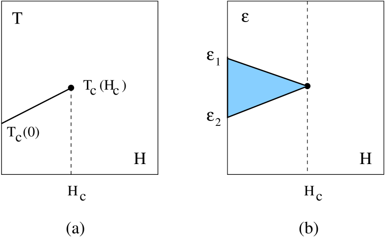
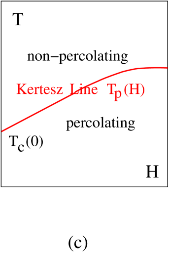
We want to show here that the equivalence of thermodynamic and geometric critical behaviour can be extended to the case $H\not=0$. Since in the case of continuous thermodynamic transitions, such as those of the Ising model, the introduction of an external field excludes singular behaviour (for the case $d=2$ this is shown analytically [9, 6]), our problem makes sense only for first order transitions, for which the discontinuity remains over a certain range of $H$, even though for $H\not=0$, the symmetry is broken. The ideal tool for such a study is the $q$-state Potts’ model on a lattice $\mathbbm{Z}^{d}$, with $q\geq 3$ and $d\geq 3$. In this case, we have a thermodynamic phase diagram of the type shown in Fig. 1a, with a line of first order transitions starting at $T_{c}(0)$ and ending at a second order point $T_{c}(H_{c})$ [10]; the transition at this endpoint is found to be in the universality class of the 3-d Ising model. In terms of the energy density $\epsilon(H)$ of the system (the energy per lattice volume), the phase diagram has the form shown in Fig. 1b; for $H=0$, the coexistence range $\epsilon_{2}\leq\epsilon(0)\leq\epsilon_{1}$ corresponds to the critical temperature $T_{c}(0)$. The average spin $m(\epsilon)$ as order parameter vanishes for $\epsilon\geq\epsilon_{1}$ and becomes finite for smaller $\epsilon$. We want to show that in the temperature range $T_{c}(0)\leq T(H)\leq T_{c}(H_{c})$, the corresponding Kertész line $T_{p}(H)$ (see Fig. 1c) coincides with that of the thermal discontinuity and that it also leads to the same first order/second order phase structure. Let us begin with a conceptual discussion of the situation.

The $q$-state Potts’ model in the absence of an external field provides $q+1$ phases: the disordered phase at high temperature and $q$ degenerate ordered low-temperature phases. Spontaneous symmetry breaking has the system fall into one of these as the temperature is decreased. Turning on a small external field $H$ aligns the spins in its direction and thus effectively removes the $q-1$ “orthogonal” low-temperature phases. Hence now only two phases remain: the ordered low-temperature state of spins aligned in the direction of $H$, and the disordered high-temperature phase. The two are for $T<T_{c}(H_{c})$ separated by a mixed-phase coexistence regime. At the endpoint $T=T_{c}(H_{c})$, there is a continuous transition from a system in one (symmetry broken) ordered phase to the corresponding (symmetric) disordered phase. The behaviour at $H=H_{c}$ in Fig. 1b is thus just that of the Ising model, and hence the endpoint transition is in its universality class.

In the geometric formulation for $H=0$, with decreasing temperature or energy density there is formation of finite clusters of $q$ different orientations; the clusters here are defined using the temperature-dependent F-K bond weights. At $\epsilon(0)=\epsilon_{1}$, the $Z_{q}$ symmetry is spontaneously broken: for one of the $q$ directions, there now are percolating clusters, and the percolation strength $P(\epsilon)$ becomes finite for $\epsilon<\epsilon_{1}$. However, the disordered phase also still forms a percolating medium (for $d\geq 3$). A further decrease of the energy density reduces the fraction of space in disordered state, and for $\epsilon(0)\leq\epsilon_{2}$, there is no more disordered percolation. Embedded in the disordered phase are at all times finite clusters of a spin orientation “orthogonal” to the one chosen by spontaneous symmetry breaking. In our treatment, we will therefore divide the set of clusters into three classes: disordered, ordered in the direction of symmetry breaking, and ordered orthogonal to the latter. While for $H=0$, any of the $q$ directions could be the given orientation, for $H\not=0$, the external field specifies the alignment direction, making the $q-1$ sets of “orthogonal” clusters essentially irrelevant. It is for this reason that at the endpoint of a line of first order transitions one generally encounters the universality class of the Ising model. Whatever the original symmetry of the system was, at the endpoint there remains only the aligned and the disordered ground states.

The plan of the paper is as follows. In the next section, we recall the cluster treatment of the Potts’ model and specify our method to identify the different cluster types. This will be followed by an analytic study valid for small external fields and by numerical calculations for different $q$ up to asymptotic values of $H$. Formal details of the analytic calculation are given in the appendix.

We consider a finite–volume $q$–state Potts model on the lattice $\mathbbm{Z}^{d}$ ($d\geq 2$), at inverse temperature $\beta=1/T$ and subject to an external ordering field $h$. It is defined by the Boltzmann weight

$$\omega_{\operatorname{Potts}}(\boldsymbol{\sigma})=\prod_{\langle i,j\rangle}e^{\beta(\delta_{\sigma_{i},\sigma_{j}}-1)}\prod_{i}e^{h\delta_{\sigma_{i},1}},$$

(1)

where the spins $\sigma_{i}$ take on the values of the set $\{1,\ldots,q\}$, and where the first product is over nearest neighbour pairs (n,n). If we want to study the behaviour of clusters, in the sense of F-K clusters, we turn to the corresponding Edwards–Sokal formulation [5], given by the Boltzmann weight

$$\omega_{\operatorname{ES}}(\boldsymbol{\sigma},\boldsymbol{\eta})=\prod_{\langle i,j\rangle}[e^{-\beta}\delta_{\eta_{ij},0}+(1-e^{-\beta})\delta_{\eta_{ij},1}\delta_{\sigma_{i},\sigma_{j}}]\prod_{i}e^{h\delta_{\sigma_{i},1}},$$

(2)

where the edge variables $\eta_{ij}$ belong to $\{0,1\}$. This “site-bond” model can be thought of as follows. Given a certain spin configuration, one puts between two neighbouring sites $\sigma_{i}=\sigma_{j}$ an edge or bond with the probability $1-e^{-\beta}$, and no edge with the probability $e^{-\beta}$; for $\sigma_{i}\neq\sigma_{j}$, no bond is present. When the field is infinite, all $\sigma_{i}=1$, and we are left with a classical bond percolation problem, while for finite field, one has a random bond percolation model in the random media given by the spin configuration.

In the presence of an external field, we find it convenient for the study of the Kertész’s line to consider a modified version of the Edwards–Sokal formulation. We have three different types of spin combination: (0) two adjacent spins $i,j$ are not equal, (1) two adjacent spins $i,j$ are equal and parallel to $h$ (we denote this direction as 1), or (2) two adjacent spins $i,j$ are equal but not parallel to $h$. Correspondingly, we “color” the edge between $i$ and $j$ in three different colors $n_{i,j}$, where the edge variables $n_{ij}$ belong to $\{0,1,2\}$. The resulting Boltzmann weight becomes

$$\omega_{\operatorname{CES}}(\boldsymbol{\sigma},\boldsymbol{n})=\prod_{\langle i,j\rangle}[e^{-\beta}\delta_{n_{ij},0}+(1-e^{-\beta})\delta_{n_{ij},1}\chi_{(\sigma_{i}=\sigma_{j}=1)}\\ +(1-e^{-\beta})\delta_{n_{ij},2}\chi_{(\sigma_{i}=\sigma_{j}\neq 1)}]\prod_{i}e^{h\delta_{\sigma_{i},1}},$$

(3)

where the characteristic function $\chi(\sigma_{i}=\sigma_{j}=1)$ is unity for $\sigma_{i}=\sigma_{j}=1$ (parallel spins in the direction of $h$) and zero otherwise, while $\chi(\sigma_{i}=\sigma_{j}\neq 1)$ is unity for parallel spins not in the direction of $h$ and zero otherwise. The summation over the spin variables then leads to the following Tricolor–Edge–Representation

$$\omega_{\operatorname{TER}}(\boldsymbol{n})=\prod_{\langle i,j\rangle}e^{-\beta\delta_{n_{ij},0}}(1-e^{-\beta})^{(\delta_{n_{ij},1}+\delta_{n_{ij},2})}\times\\ e^{hS_{1}(\boldsymbol{n})}(q-1)^{C_{2}(\boldsymbol{n})}(q-1+e^{h})^{|\Lambda|-S_{1}(\boldsymbol{n})-S_{2}(\boldsymbol{n})}.$$

(4)

Here, $S_{1}(\boldsymbol{n})$ and $S_{2}(\boldsymbol{n})$ denote the number of sites that belong to edges of color $1$ and color $2$, respectively, while $C_{2}(\boldsymbol{n})$ denotes the number of connected components of the set of edges of color $2$, and $|\Lambda|$ is the number of sites of the lattice under consideration.

Let us mention that such kind of graphical representation has already been considered for various spin models in presence of an external field [3].

Let $p_{\Lambda}(i\leftrightarrow j)$ be the probability that the site $i$ is connected to $j$ by a path of edges of color $1$. As (geometric) order parameter we will consider the following mass–gap (inverse correlation length)

$$m(\beta,h)=-\lim_{|i-j|\rightarrow\infty}\frac{1}{|i-j|}\ln\lim_{\Lambda\uparrow\mathbbm{Z}^{d}}p_{\Lambda}(i\leftrightarrow j)$$

(5)

where $i$ and $j$ belong to some line parallel to an axis of the lattice. As (thermodynamic) order parameter, we shall consider the mean energy $E(\beta,h)=-\frac{1}{\beta}\frac{\partial}{\partial\beta}f(\beta,h)$, where $f(\beta,h)$ is the free energy of the model ⁴⁴4 Note that all partitions functions, and hence the free energies, of models (1 )–(4 ) coincide .

Let us first have a look at the diagram of ground state configurations of the TER representation which are the translation invariant configurations maximizing the Boltzmann weight (4).

For the color $a=0,1,2$, let $b_{a}$ be the value of the Boltzmann weight of the ground state configuration of color $a$ per unit site. One finds $b_{0}=e^{-\beta d}(q-1+e^{h}),b_{1}=(1-e^{-\beta})^{d}e^{h},b_{2}=(1-e^{-\beta})^{d}$.

Notice that $b_{0}=b_{1}$ on the line

$$\beta_{0}(h)=\ln[1+(1+(q-1)e^{-h})^{1/d}]$$

(6)

and that $b_{0}=b_{1}=b_{2}$ at the point $\beta_{0}(0)$.

The diagram of ground state configurations, inferred from the values of the weights $b_{0},b_{1},b_{2}$ is shown in Fig. 2 (in the $(h,\beta)$ plane).

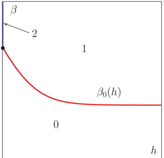
When $q$ is large enough and $h$ not too large, the TER representation (4) can be analyzed rigorously by a perturbative approach. Namely, by using the standard machinery of Pirogov–Sinai theory, we will show that the model undergoes a thermodynamic first order phase transition in the sense that the mean energy (as well as the magnetization) is discontinuous at some $\beta_{c}(h)\sim\beta_{0}(h)$. We also find for these values of the parameters, that the phase diagram of this model reproduces the diagram of ground state configurations (Fig. 2), see Appendix for more details.

In addition, the model exhibits a geometric (first order) transition, in the sense that, on the same critical line, the mass gap is discontinuous.

The proof is given in the appendix.

Let us recall that it has already been shown that the Potts model (1) undergoes, for $q$ large and $h$ small, a first order phase transition on a critical line [1], where both the mean energy and the magnetization are discontinuous. Since, as already mentioned, the free energies of models (1) and (4) are the same, this critical line coincides with the one mentioned in the theorem.

In the absence of an external magnetic field, the statements of the theorem have been shown previously [13, 14, 12].

Condition (7) restricts the range of values of parameters to which our rigorous analysis applies. Moreover, we do not expect thermodynamic first order transitions when $h$ is sufficiently enhanced. In the next section, we turn to numerical study on a wider range of values.

We have implemented a generalization of the Swendsen–Wang algorithm for our colored Edwards–Sokal model (3).

First, given a spin configuration, we put between any two neighbouring spins of the same color, an edge colored $0$ with probability (w.p.) $e^{-\beta}$, and w.p. $1-e^{-\beta}$, an edge colored $1$ if these spins are of color $1$, and colored $2$ otherwise. When two neighbouring spins disagree, the corresponding edge is colored $0$.

Then, starting from an edge configuration, a spin configuration is constructed as follows. Isolated sites (endpoints of $0$–bonds only) are colored $1$ w.p. $e^{h}/(q-1+e^{h})$ and colored $c\in\{2,...,q\}$ w.p. $1/(q-1+e^{h})$. Non–isolated sites are colored $1$ (w.p. 1) if they are endpoints of $1$–bonds and colored $c\in\{2,...,q\}$ w.p. $1/(q-1)$.

This algorithm allows us two compute both quantities associated to spins configurations and those associated to edges configurations.

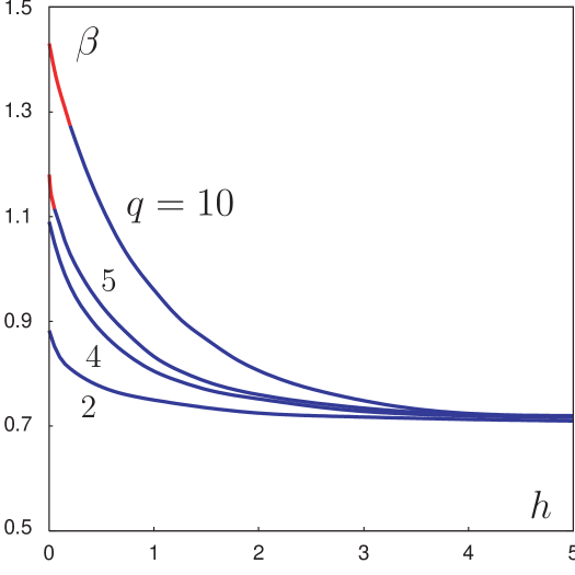
The numerical results for $d=2$ are presented in Fig. 3. For $q\leq 4$, we found a whole geometric transition line $\beta_{c}(h)$ for which $m(\beta,h)>0$ when $\beta<\beta_{c}(h)$, and $m(\beta,h)=0$ when $\beta\geq\beta_{c}(h)$. The mass gap is continuous at $\beta_{c}(h)$. For $\beta<\beta_{c}(h)$, the mean cluster sizes remain finite, while for $\beta\geq\beta_{c}(h)$ the size of $1$–edge clusters diverges. The energy density as well as the magnetization do not show any singular behavior.

For $q\geq 5$, some critical $h_{c}$ appears for which the geometric transition line $\beta_{c}(h)$ becomes first order when $h<h_{c}$, i.e. $m(\beta,h)>0$ for $\beta\leq\beta_{c}(h)$ and $m(\beta,h)=0$ for $\beta>\beta_{c}(h)$. In addition, on this part of the line, we find that the mean energy is discontinuous ⁵⁵5The Swendsen-Wang algorithm allows to compute both associated order parameters (mass-gap and mean energy).. When $h\geq h_{c}$, only a geometric transition occurs and the scenario is the same as for $q\leq 4$. Thus our numerics show that the geometric and thermodynamic transitions coincide up to $h_{c}$, similarly to what we got analytically but only at (very) small field (and large $q$), see Fig. 3.

Let us mention that the numerics are in accordance with the theory for vanishing and infinite fields: $\beta_{c}(0)=\ln(1+\sqrt{q})$ and $\beta_{c}(\infty)=\ln 2$.

The system size in these calculations was $L=50$, $d=2$. The “first order” part of the transition lines has been determined via Binder cumulants [2]. The Hoshen-Kopelman algorithm [8] was used to study cluster statistics. For each value of $q$, more than $2\times 10^{5}$ iterations were performed. Data have been binned in order to control errors in measurements.

For the Potts model in the presence of an external magnetic field, we have shown that when the Kertész line is first order, it coincides with the usual thermodynamic critical line. This property holds up to some critical point $(h_{c},\beta_{c}(h_{c}))$, beyond which the thermodynamic transition disappears. Such behavior may well appear also for a broader class of models exhibiting first order transition in the presence of an external field. We believe that the behavior at the above critical point also belongs to the universality class of the Ising model, as it is the case in the $3$–state Potts model in three dimensions [10].

It is a pleasure to thank János Kertész for interesting comments. The BIBOS research center (Bielefeld) and the Centre de Physique Théorique (CNRS Marseille) are gratefully acknowledged for warm hospitality and financial support. The authors are indebted to an anonymous referee for constructive remarks.

We first introduce the partition function of the TER representation with boundary conditions $a\in\{0,1,2\}$ in a box $\Lambda$ ⁶⁶6The reader should not be confused by the fact that (8), called diluted partition function in PS–theory, differs from the usual one by an unimportant boundary term which makes the expansions (10) and (11) easier to write.:

$$Z_{a}(\Lambda)=\sum_{\boldsymbol{n}}\prod_{i\in\Lambda}\omega_{i}(\boldsymbol{n})q^{C_{2}(\boldsymbol{n})-\delta_{a,2}}\prod_{i\in\partial\Lambda}\prod_{j\sim i}\delta_{n_{ij},a}$$

(8)

where the sum is over all configurations $\boldsymbol{n}=\{n_{ij}\}_{ij\cap\Lambda\emptyset}$, $\partial\Lambda$ is the boundary of $\Lambda$ (set of sites of $\Lambda$ with a n.n. in $\mathbbm{Z}^{d}\setminus\Lambda$), the notation $i\sim j$ means that $i$ and $j$ are n.n., and

$$\omega_{i}(\boldsymbol{n})=(1-e^{-\beta})^{(\delta_{n_{ij},1}+\delta_{n_{ij},2})/2}e^{-\beta\delta_{n_{ij},0}/2}e^{h\chi(i\in``1^{\prime\prime})}(q-1+e^{h})^{\prod_{j\sim i}\delta_{n_{ij},0}}$$

(9)

where $\chi(i\in``1^{\prime\prime})$ means that the site $i$ belongs to some edge of color $1$. Next, consider a configuration$\boldsymbol{n}$ on the envelope of $\Lambda$: $E(\Lambda)=\{\langle i,j\rangle\cap\Lambda\neq\emptyset\}$. A site $i\in\Lambda$ is called correct if for all $j\sim i$, $n_{ij}$ takes the same value, and called incorrect otherwise. Denote $I(\boldsymbol{n})$ the set of incorrect sites of the configuration $\boldsymbol{n}$. A couple $\Gamma=\{\operatorname{Supp}\Gamma,\boldsymbol{n}(\Gamma)\}$ where the support of $\Gamma$ ($\operatorname{Supp}\Gamma$) is a maximal connected subset of $I(\boldsymbol{n})$, and $\boldsymbol{n}(\Gamma)$ the restriction of $\boldsymbol{n}$ to the envelope of $\Lambda$ is called contour of the configuration $\boldsymbol{n}$ (here, a set of sites is called connected if the graph that joins all the sites of this set at distance $d(i,j)=\max_{k=1,\ldots,d}|i_{k}-j_{k}|\leq 1$ is connected). A couple $\Gamma=\{\operatorname{Supp}\Gamma,\boldsymbol{n}(\Gamma)\}$ where $\operatorname{Supp}\Gamma$ is a connected set of sites is called contour if there exists a configuration $\boldsymbol{n}$ such that $\Gamma$ is a contour of $\boldsymbol{n}$. For a contour $\Gamma$, let $\boldsymbol{n}_{\Gamma}$ denote the configuration having $\Gamma$ as unique contour, $\operatorname{Ext}\Gamma$ denotes the unique infinite component of $\mathbbm{Z}^{d}\setminus(\operatorname{Supp}\Gamma)$, $\operatorname{Int}\Gamma=\mathbbm{Z}^{d}\setminus(\operatorname{Ext}\Gamma\cup\operatorname{Supp}\Gamma)$, and $\operatorname{Int}_{m}\Gamma$ denote the set of sites of $\operatorname{Int}\Gamma$ corresponding to the color $m\in\{0,1,2\}$ for the configuration $\boldsymbol{n}_{\Gamma}$. Two contours $\Gamma_{1}$ and $\Gamma_{2}$ are said to be compatible if their union is not connected and are called external contours if furthermore $\operatorname{Int}\Gamma_{1}\subset\operatorname{Ext}_{\Lambda}\Gamma_{2}$ and $\operatorname{Int}\Gamma_{2}\subset\operatorname{Ext}_{\Lambda}\Gamma_{1}$. For a family $\theta=\{\Gamma_{1},\ldots,\Gamma_{n}\}_{\operatorname{ext}}$ of external contours, let $\operatorname{Ext}_{\Lambda}\theta$ denote the intersection $\Lambda\cap_{k=1}^{n}\operatorname{Ext}_{\Lambda}\Gamma_{k}$. With these definitions and notations, one gets the following expansion of the partition functions over families of external contours,

$$Z_{a}(\Lambda)=\sum_{\theta=\{\Gamma_{1},\ldots,\Gamma_{n}\}_{\operatorname{ext}}}b_{a}^{|\operatorname{Ext}_{\Lambda}\theta|}\prod_{k=1}^{n}\rho(\Gamma_{k})\prod_{\text{$m=0,1,2$}}Z_{m}(\operatorname{Int}_{{}_{m}}\Gamma_{k}),$$

(10)

where $\rho(\Gamma)=\prod_{i\in\operatorname{supp}\Gamma}\omega_{i}(\boldsymbol{n}_{\Gamma})q^{C(\boldsymbol{n}_{\Gamma})-\delta_{a,2}}$. From (10), we get

$$Z_{a}(\Lambda)=b_{a}^{|\Lambda|}\sum_{\{\Gamma_{1},\ldots,\Gamma_{n}\}_{\operatorname{comp}}}\prod_{k=1}^{n}z_{a}(\Gamma_{k}),$$

(11)

where the sum is now over families of compatible contours and the activities $z_{a}(\Gamma)$ of contours are given by $z_{a}(\Gamma)=\rho(\Gamma)b_{a}^{-|\operatorname{supp}\Gamma|}\prod_{m\neq a}\frac{Z_{m}(\operatorname{Int}_{{}_{m}}\Gamma)}{Z_{a}(\operatorname{Int}_{{}_{m}}\Gamma)}$.

It is easy to prove the following Peierls’ estimate,

$$\rho(\Gamma)(\max_{a=0,1,2}b_{a})^{-|\operatorname{Supp}\Gamma|}\leq e^{-\tau|\operatorname{Supp}\Gamma|},$$

(12)

where $e^{-\tau}=(1+(q-1)e^{-h})^{-1/2d}$. Indeed, first notice that an incorrect site $i$ is either of color $1$ or of color $2$. In the first case one has $\sum_{j\sim i}(\delta_{n_{ij},0}+\delta_{n_{ij},1})=2d$, so that $\omega_{i}(\boldsymbol{n}_{\Gamma})/b_{1}=(e^{\beta}-1)^{-(\sum_{j\sim i}\delta_{n_{ij},0})/2}$, implying

$$\omega_{i}(\boldsymbol{n}_{\Gamma})/\max_{a=0,1,2}b_{a}\leq(1+(q-1)e^{-h})^{-(\sum_{j\sim i}\delta_{n_{ij},0})/2d}.$$

Thus since $1\leq\sum_{j\sim i}\delta_{n_{ij},0}\leq 2d-1$, each incorrect site of color $1$ gives at most a contribution $e^{-\tau}$ to the L.H.S. of (12). In the second case, one has $\sum_{j\sim i}(\delta_{n_{ij},0}+\delta_{n_{ij},2})=2d$, so that $w_{i}(\boldsymbol{n}_{\Gamma})/b_{2}=(e^{\beta}-1)^{-(\sum_{j\sim i}\delta_{n_{ij},0})/2},$ implying

$$\omega_{i}(\boldsymbol{n}_{\Gamma})/\max_{a=0,1,2}b_{a}\leq(q-1+e^{h})^{-(\sum_{j\sim i}\delta_{n_{ij},0})/2d}.$$

We then use again that $1\leq\sum_{j\sim i}\delta_{n_{ij},0}\leq 2d-1$ and that $C_{2}(\boldsymbol{n}_{\Gamma})\leq\sum_{i\in\operatorname{Supp}\Gamma}\chi(1\leq\delta_{n_{ij},2})/2^{\sum_{j\sim i}\delta_{n_{ij},2}}$ (see [12]) to obtain that each incorrect site of color $2$ gives at most a contribution $(e^{h}+q-1)^{-1/2+1/2d}\leq e^{-\tau}$ to the L.H.S. of (12).

When the assumptions of the theorem are satisfied, the Peierls’ estimate (12) provides a good control of the system by using Pirogov–Sinai theory [15]. We introduce the truncated activity

$$z_{a}^{\prime}(\Gamma)=\left\{\begin{array}[]{l}z_{a}(\Gamma)\operatorname{if}z_{a}(\Gamma)\leq(c_{0}e^{-\tau})^{|\operatorname{Supp}\Gamma|}\\ (c_{0}e^{-\tau})^{|\operatorname{Supp}\Gamma|}\operatorname{otherwise,}\end{array}\right.$$

where $c_{0}$ is a numerical constant, and we call a contour stable if $z_{a}(\Gamma)=z_{a}^{\prime}(\Gamma)$. Let $Z_{a}^{\prime}(\Lambda)$ be the partition function obtained from (11) by leaving out unstable contours, i.e., by taking the activities $z_{a}^{\prime}(\Gamma)$ in (11), and let us introduce the metastable free energies $f^{\operatorname{met}}_{a}(\beta,h)=-\lim_{\Lambda\uparrow\mathbbm{Z}^{d}}(1/|\Lambda|)\ln Z_{a}^{\prime}(\Lambda)$. The leading term of these metastable free energies equals $-\ln b_{a}$. The corrections can be expressed by free energies of contour models which can be controlled by convergent cluster expansions. As a standard result of Pirogov-Sinai theory, one gets that the phase diagram of the system is a small perturbation of the diagram of ground state configurations. Namely, there exits a unique point $\beta_{c}(0)$ given by the solution of $f_{0}^{\operatorname{met}}(\beta,h)=f_{1}^{\operatorname{met}}(\beta,h)=f_{2}^{\operatorname{met}}(\beta,h)$ for which all contours are stable and such that $Z_{a}(\Lambda)=Z_{a}^{\prime}(\Lambda)$ for $a=0,1,2$. There exists a line $\beta_{c}(h)$ given by the solution of $f_{0}^{\operatorname{met}}(\beta,h)=f_{1}^{\operatorname{met}}(\beta,h)$ when $h>0$ and such that, $Z_{a}(\Lambda)=Z_{a}^{\prime}(\Lambda)$ for $a=0,1$. For $\beta<\beta_{c}(h)$ one has $Z_{0}(\Lambda)=Z_{0}^{\prime}(\Lambda)$, and for $\beta>\beta_{c}(h)$ one has $Z_{1}(\Lambda)=Z_{1}^{\prime}(\Lambda)$. For $h=0$ and $\beta\geq\beta_{c}(0)$, one has in addition $Z_{2}(\Lambda)=Z_{2}^{\prime}(\Lambda)$.

For the color $a=0,1,2$, denote by $\langle\cdot\rangle^{a}(\beta,h)$ the expectation value under the $a$–boundary condition. As a consequence of the above expansions and analysis, we obtain by standard Peierls’ estimates that for $h\geq 0$

	$\displaystyle\langle\delta_{n_{ij},1}\rangle^{1}(\beta,h)$	$\displaystyle\geq$	$\displaystyle 1-O(e^{-\tau})\quad\text{for}\quad\beta\geq\beta_{c}(h)$		(13)
	$\displaystyle\langle\delta_{n_{ij},0}\rangle^{0}(\beta,h)$	$\displaystyle\geq$	$\displaystyle 1-O(e^{-\tau})\quad\text{for}\quad\beta\leq\beta_{c}(h)$		(14)

while in addition we also get for $h=0$:

$$\langle\delta_{n_{ij},2}\rangle^{2}(\beta,0)\geq 1-O(e^{-\tau})\quad\text{for}\quad\beta\geq\beta_{c}(0)$$

(15)

By definition of the mean energy, one has that $\Delta E=E(\beta^{-},h)-E(\beta^{+},h)$ is proportional to the difference $\langle\delta_{n_{ij},0}\rangle^{0}(\beta^{-},h)-\langle\delta_{n_{ij},0}\rangle^{1}(\beta,h)$, and the first statement of the theorem follows immediately from these properties.

To prove the second statement, we remark that if one imposes that the site $i$ is connected to $j$ by a path made up of edges of color $1$, then under the boundary condition $0$, there exists necessarily an external contour that encloses both the sites $i$ and $j$. As a consequence of the above analysis the probability of external contours $\Gamma$ decays like $(c_{0}e)^{-\tau|\operatorname{Supp}\Gamma|}$ when the $0$–contours are stable, i.e. when $Z_{0}(\Lambda)=Z_{0}^{\prime}(\Lambda)$. One thus gets $p_{\Lambda}(i\leftrightarrow j)\leq(\operatorname{Cte}e^{-\tau})^{|i-j|}$ when $\beta\leq\beta_{c}(h)$ from which the first statement of the theorem follows. On the other hand under the boundary condition $1$, the probability that the site $i$ is not connected to $j$ can be bounded from above by a small number $O(e^{-\tau})$ when $Z_{1}(\Lambda)=Z_{1}^{\prime}(\Lambda)$. This follows also from a Peierls type arguments and implies that the probability that the site $i$ is connected to $j$ under the boundary condition $1$ is greater than $1-0(e^{-\tau})$ for $\beta\geq\beta_{c}(h)$. It gives also that the probability $p_{\Lambda}(i\leftrightarrow j)$ for the site $i$ to be connected with $j$ under the boundary condition $0$ is also greater than $1-0(e^{-\tau})$ for $\beta>\beta_{c}(h)$, implying the second statement.

References

- [1] A. Bakchich, A. Benyoussef, and L. Laanait, Ann. Inst. Henri Poincaré, 50:17, 1989.
- [2] K. Binder and D. P. Landau, Phys. Rev., B30,3:1477, 1984; M.S.S. Challa, K. Binder, and D. P. Landau, Phys. Rev., B34,3:1841, 1986;
- [3] L. Chayes and J. Machta, Physica A, 239:542, 1997.
- [4] A. Coniglio, W. Klein, J. Phys. A 13, 2775 (1980).
- [5] R.G. Edwards and A.D. Sokal, Phys. Rev. D, 38:2009, 1988.
- [6] S. Friedli and C.–E. Pfister, Phys. Rev. Lett. 92, 015702 (2004), Comm. Math. Phys. 245, 69 (2004).
-
[7]
C. M. Fortuin, P. W. Kasteleyn,
J. Phys. Soc. Japan 26 (Suppl.), 11 (1969);
Physica 57, 536 (1972). - [8] J. Hoshen and R. Kopelman Phys. Rev., B14,8:3438, 1976.
- [9] S. N. Isakov, Comm. Math. Phys. 95, 427 (1984).
- [10] F. Karsch and S. Stickan, Phys. Lett. B 488 (2000) 319.
- [11] J. Kertész, Physica A 161, 58 (1989).
- [12] R. Kotecký, L. Laanait, A. Messager, and J. Ruiz. J. Stat. Phys., 58:199, 1990.
- [13] L. Laanait, A. Messager, S. Miracle–Solé, J. Ruiz, and S. Shlosman, Commun. Math. Phys., 140:81, 1991.
- [14] L. Laanait, A. Messager, and J. Ruiz, Commun. Math. Phys., 105:527, 1986.
- [15] Ya. G. Sinai, Theory of Phase Transitions: Rigorous Results, Pergamon Press, London, 1982; M. Zahradník, Commun. Math. Phys., 93:359, 1984;