On the Laplacian spectrum of $k$-symmetric graphs

A simple graph $G=(V,E)$ is a combinatorial object consisting of a finite set $V$ and a set $E$ of unordered pairs of different elements of $V$. The elements of $V$ and $E$ are called the vertices and the edges of the graph $G$, respectively. For a given graph $G$, the vertex set and the edge set of $G$ are denoted by $V(G)$ and $E(G)$, respectively.

Let $G$ be a graph with enumerated vertices. The Laplacian matrix $L(G)$ of $G$ is defined as $L(G)=D(G)-A(G)$, where $D(G)$ is the diagonal matrix of vertex degrees and $A(G)$ is the adjacency matrix of $G$. Thus the Laplacian matrix is symmetric. Note that the Laplacian matrix can be considered a positive-semidefinite quadratic form on the Hilbert space generated by $V(G)$. Since the Laplacian matrix contains information on the structure of the graph, it has been studied importantly in various applied fields including artificial neural network research using graph shaped data [13, 14].

Let $G$ be a graph with $n$ vertices. For a square matrix $M$, we denote the characteristic polynomial of $M$ by $\mu(M,x)$. A root of the characteristic polynomial of Laplacian matrix $L(G)$ is called a Laplacian eigenvalue of $G$. Denote the all eigenvalues of $L(G)$ by $\lambda_{n}(G)\leq\lambda_{n-1}(G)\leq\cdots\leq\lambda_{1}(G)$. It is well-known that $\lambda_{n}(G)=0$ and $\lambda_{1}(G)\leq n$. The multiset of Laplacian eigenvalues of $G$ is called the Laplacian spectrum of $G$. The Laplacian spectrum of the complement graph $\overline{G}$ of $G$ is satisfying

The Laplacian spectrum shows us several properties of the graph. For instance, Kirchhoff [15] proved that the number of spanning tree of a connected graph $G$ with $n$ vertices is $\frac{1}{n}\lambda_{1}(G)\cdots\lambda_{n-1}(G)$. Let $m_{G}(\lambda)$ denote the multiplicity of $\lambda$ as a Laplacian eigenvalue of $G$. Note that the multiplcity of 0 is equal to the number of connected components of $G$.

The connectivity $\kappa(G)$ of a graph $G$ is the minimum number of vertices whose removal results in a disconnected or trivial graph. A graph $G$ is said to be $t$-connected if $\kappa(G)\geq t$. If a graph is $t$-connected, then it is $(t\!-\!1)$-connected. Fiedler [9] proved that the second smallest Laplacian eigenvalue of $G$ is less than or equal to $\kappa(G)$.

A pendant vertex of $G$ is a vertex of degree $1$. A quasi-pendant of $G$ is a vertex adjacent to a pendant. We denote the number of pendants of $G$ by $p(G)$, and the number of quasi-pendant vertices by $q(G)$. In [8], Faria showed that for any graph $G$,

It implies that if $p(G)$ is greater than $q(G)$, then $G$ has a Laplacian eigenvalue 1. Also, such graph $G$ is at most 1-connected. In [1], Barik et al. found trees with a Laplacian eigenvalue 1 even though the right-hand side of the above inequality is 0. Since a tree has connectivity 1, we focus on 2-connected graph with a Laplacian eigenvalue 1.

The simplest way to obtain a 2-connected graph with a Laplacian eigenvalue 1 is the Cartesian product. The Cartesian product $G\square H$ of graphs $G$ and $H$ is the graph with the vertex set $V(G)\times V(H)$ such that two vertices $(v,v^{\prime})$ and $(w,w^{\prime})$ are adjacent if $v=w$ and $v^{\prime}$ is adjacent to $w^{\prime}$ in $H$, or if $v^{\prime}=w^{\prime}$ and $v$ is adjacent to $w$ in $G$. Fiedler [9] showed that the Laplacian eigenvalues of the Cartesian product $G\square H$ are all possible sums of Laplacian eigenvalues of $G$ and $H$. If either $G$ or $H$ has a Laplacian eigenvalue 1, then 1 is a Laplacian eigenvalue of $G\square H$. Špacapan [20] showed that the connectivity of $G\square H$ is

where $\delta(G\square H)$ is the minimum degree of $G\square H$. Remark that if $G$ and $H$ are connected graphs, then $G\square H$ is 2-connected. Thus we concentrate a 2-connected graph that does not decompose nontrivial graphs under the Cartesian product. If a graph does not admit the nontrivial Cartesian product decomposition, then the graph is called prime with respect to the Cartesian product. In this paper, we prove the following theorem.

Meanwhile, integral spectra of Laplacian matrix or adjacency matrix are studied in various application fields including physics and chemistry [3, 4, 5]. A graph with integral Laplacian spectrum is called a Laplacian integral graph. If a graph does not include the path $P_{4}$ as an induced subgraph, then it is called a cograph. In [19], Merris showed that a cograph is a Laplacian integral graph. Many researchers [7, 10, 16, 17] have investigated infinitely many classes of Laplacian integral graphs that are not cographs. In section 5, we introduce a new graph $\mathcal{C}(n,m)$ for some positive integers $n$ and $m$. The graph $\mathcal{C}(n,m)$ is obtained by connecting several set of vertices for $m$ parallel copies of $n$-complete graph $K_{n}$ to the corresponding vertex of $\overline{K}_{n}$. Later, we examine that if $n\geq 2$, then $\mathcal{C}(n,m)$ has the path $P_{4}$ as the induced subgraph, that is, it is not a cograph. In this paper, we also prove the following theorem.

This paper is organized as follows. In Section 2, We provide some linear algebra results needed for proof of main theorems. In Section 3, We define the $k$-symmetric graph by relaxing the condition of symmetric graph, and examine its properties. In Section 4 and Section 5, we prove the main theorems and related properties.

In this section, we introduce some definitions and properties that will be used in this paper. The set of all $m\times n$ matrices over a field $\mathbb{F}$ is denoted by $M_{m\times n}(\mathbb{F})$. Denote $M_{n\times n}(\mathbb{F})$ by $M_{n}(\mathbb{F})$. We denote by $I_{n}$ and $J_{n}$ the $n\times n$ identity matrix and the $n\times n$ matrix whose entries are ones. Also, $1_{n}$ is the $n$-vector of all ones.

Let $A\in M_{n}(\mathbb{F})$ be a block matrix of the form

where $A_{11}\in M_{m}(\mathbb{F})$, $A_{12}\in M_{m\times(n-m)}(\mathbb{F})$, $A_{21}\in M_{(n-m)\times m}(\mathbb{F})$ and $A_{22}\in M_{n-m}(\mathbb{F})$. It is well known that if $A_{22}$ is invertible, then $\det{A}=\det{A_{22}}\det(A_{11}-A_{12}A_{22}^{-1}A_{21})$ (see [12, Chapter 0]).

For two matrices $A=(a_{ij})\in M_{m\times n}(\mathbb{F})$ and $B\in M_{p\times q}(\mathbb{F})$, the Kronecker product of $A$ and $B$, denoted by $A\otimes B$, is defined as

We state some basic properties of the Kronecker product (for more details, see [11, Chapter 4]):

• (a)

  $A\otimes(B+C)=A\otimes B+A\otimes C$.

• (b)

  $(B+C)\otimes A=B\otimes A+C\otimes A$.

• (c)

  $(A\otimes B)(C\otimes D)=AC\otimes BD$.

• (d)

  If $A\in M_{m}(\mathbb{F})$ and $B\in M_{n}(\mathbb{F})$ are invertible, then $(A\otimes B)^{-1}=A^{-1}\otimes B^{-1}$.

• (e)

  $\det(A\otimes B)=(\det{A})^{n}(\det{B})^{m}$ for $A\in M_{m}(\mathbb{F})$ and $B\in M_{n}(\mathbb{F})$.

A matrix $T\in M_{n}(\mathbb{F})$ of the form

is called a Toeplitz matrix. In [18], the authors gave a Toeplitz matrix inversion formula.

Symmetry is an important property of graphs. We deal with graphs that has symmetric property. Let $G$ be a graph. An automorphism $\varphi$ of a graph $G$ is a permutation of $V(G)$ such that $\varphi(v)$ and $\varphi(w)$ are adjacent if and only if $v$ and $w$ are adjacent where $v$ and $w$ are vertices of $G$. The set of all automorphisms of $G$ is called an automorphism group of $G$ and denoted by $\text{Aut}(G)$. A graph $G$ is symmetric if $\text{Aut}(G)$ acts transitively on both vertices of $G$ and ordered pairs of adjacent vertices. This implies that $G$ is regular, that is, all vertices have the same degree. However, it is a very difficult problem to determine whether a given graph is a symmetric graph. Thus we concentrate the cyclic part of $\text{Aut}(G)$. In this section, we define $k$-symmetric graphs and give some their properties. Also, we construct a $k$-symmetric graph from other $k$-symmetric graphs.

The above definition tells us that all graphs are 1-symmetric because the trivial group freely acts on any graph. If a graph $G$ with $n$ vertices is $n$-symmetric, then the automorphism group $\text{Aut}(G)$ has a cyclic subgroup $\mathcal{H}$ which transitively acts on vertices. Thus $G$ is regular. However, the converse is not true even though $G$ is a symmetric graph. Before examining this, we check the following proposition.

For example, the Petersen graph in Figure 1 is 5-symmetric because the 5-fold rotation satisfies the 5-symmetric automorphism condition. The Petersen graph is a symmetric graph with 10 vertices. But since the Petersen graph is not Hamiltonian, it is not 10-symmetric. For any positive integer $k$, $k$-symmetric graphs are satisfying the following properties.

Let $\varphi$ be a $k$-symmetric automorphism of a graph $G$ and let $\operatorname{id}_{H}$ be the identity automorphism of a graph $H$. Then the automorphism $\varphi\times\operatorname{id}_{H}$ of $G\square H$ is $k$-symmetric. Thus we obtain the following proposition.

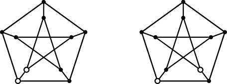
Let $G$ be a graph with a $k$-symmetric automorphism $\varphi$. Then $\mathbb{Z}_{k}$ acts on $V(G)$ as follows. For any $i\in\mathbb{Z}_{k}$ and $v\in V(G)$, we define $i\cdot v=\varphi^{i}(v)$. For any vertex $v$, the orbit of $v$ is denoted by $\mathbb{Z}_{k}\cdot v$. Let $B_{\varphi}$ be a minimal subset of $V(G)$ such that

Alternatively, $B_{\varphi}$ is a minimal subset of $V(G)$ such that

The set $B_{\varphi}$ is called a base of $\varphi$. Since $k$ choices are possible for each orbit, $B_{\varphi}$ is not unique as drawn in Figure 1. Note that the size of the base $B_{\varphi}$ is $\frac{|V(G)|}{k}$.

Now we introduce how to construct a $k$-symmetric graph from other $k$-symmetric graphs for any positive integer $k$. First we observe a graph join. Let $H_{1}$ and $H_{2}$ be graphs. The graph join $H_{1}\!\vee\!H_{2}$ of $H_{1}$ and $H_{2}$ is a graph obtained by joining each vertex of $H_{1}$ to all vertices of $H_{2}$. Since every graph is 1-symmetric with respect to identity map, we can understand graph join $H_{1}\!\vee\!H_{2}$ as a join of the bases $V(H_{1})$ and $V(H_{2})$ of $\operatorname{id}_{H_{1}}$ and $\operatorname{id}_{H_{2}}$. From this fact, we generalize graph join.

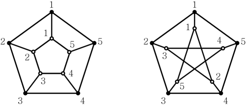
The $k$-symmetric join preserves the $k$-symmetry. Because the $k$-symmetric automorphism of $G_{1}\vee_{k}G_{2}$ is $\varphi_{1}+\varphi_{2}$ and its base is $B_{1}\cup B_{2}$. Definition 3.6 derives that the graph join is the 1-symmetric join. Note that, $n$-symmetric joins are not unique even if the base of each $G_{i}$ is unique. For instance, the Cartesian product of 5-cycle $C_{5}$ with $K_{2}$ and the Petersen graph are both 5-symmetric joins of two 5-cycles, but they are not isomorphic as drawn in Figure 2.

In this section, we prove Theorem 1.1. First we consider the multiplicity of an integral Laplacian eigenvalue. Recall that for a given graph $G$, the partition $\pi=(V_{1},V_{2},\cdots,V_{k})$ of $V(G)$ is an equitable partition if for all $i,j\in\{1,2,\ldots,k\}$ and for any $v\in V_{i}$ the number $d_{ij}=|N_{G}(v)\cap V_{j}|$ depends only on $i$ and $j$. The $k\times k$ matrix $L^{\pi}(G)=(b_{ij})$ defined by

is called the divisor matrix of $G$ with respect to $\pi$.

In the following theorem, we obtain the multiplicity of $n$ of $k$-symmetric join of graphs where $n$ is the size of a base.

If each $G_{i}$ in the above theorem is $n$-symmetric graph with $n$ vertices, then the size of a base of $G$ is $l$.

Let $G$ be an $n$-symmetric graph with $n$ vertices. Take an $n$-symmetric automorphism $\varphi$ of $G$. Let $G^{\prime}$ be a graph that $n$-symmetric join of $m$ copies of $G$ along $\varphi$. Then since each base of the copy of $G$ is a vertex, the base of $G^{\prime}$ induces the $m$ complete graph $K_{m}$. Since $G^{\prime}$ is constructed by same $n$-symmetric automorphism, $G^{\prime}$ becomes the Cartesian product of $G$ and $K_{m}$.

By the Špacapan’s result [20] about the connectivity of the Cartesian product in Section 1, we realize that for any positive integer $m$, there is a $m$-connected graph $G$ with $m_{G}(m)\geq m-1$.

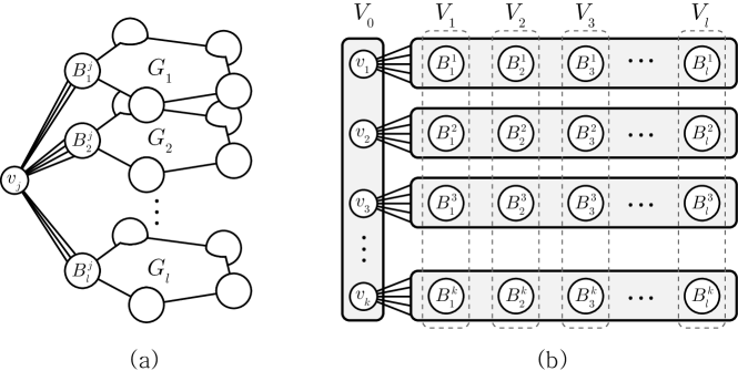
Now consider a special case of $k$-symmetric join. For any $i\in\{1,\dots,l\}$, let $G_{i}$ be a $k$-symmetric graph for some positive integer $k$ and let $\varphi_{i}$ be an associated $k$-symmetric automorphism. Let $B^{1}_{i}$ be a base of $G_{i}$, and let $B^{j}_{i}=\varphi^{j}_{i}(B^{1}_{i})$. Racall that the union of $G_{1},\dots G_{l}$ is also $k$-symmetric with the $k$-symmetric automorphism $\varphi_{1}+\cdots+\varphi_{l}$ and the base $B^{1}_{1}\cup\cdots\cup B^{1}_{l}$. Define a graph $G$ by $k$-symmetric joining $\overline{K}_{k}$ and $G_{1}\cup\cdots\cup G_{l}$. Then the subgraph induced by a base of $G$ has a cut-vertex as drawn in Figure 3 (a). From this fact, we can take an equitable partition $\pi=(V_{0},V_{1},\ldots,V_{l})$ where $V_{0}=V(\overline{K}_{k})$ and $V_{i}=V(G_{i})$ for any $i\in\{1,\dots,l\}$ as drawn in Figure 3 (b). Remark that for any distinct $i$ and $i^{\prime}$, there is no edge connecting two subgraphs $G_{i}$ and $G_{i^{\prime}}$ in $G$. To prove Theorem 1.1, we need the following two theorems.

Theorems 4.5 and 4.6 imply Theorem 1.1. Note that, if one of the graphs $G_{1},\ldots,G_{l}$ is disconnected, then there is a counterexample. For example, if $G_{1}$ is $\overline{K}_{k}$, then $G=\overline{K}_{k}\vee_{k}\left(G_{1}\cup\cdots\cup G_{l}\right)$ has a cut vertex.

In this section, we discuss $k$-symmetric graphs with integral Laplacian spectrum. Let $n$ and $m$ be positive integers. Since the $n$-complete graph $K_{n}$ is $n$-symmetric, the disjoint union of $m$ copies of $K_{n}$, denoted by $mK_{n}$, is also $n$-symmetric. We consider the $n$-symmetric join of $\overline{K}_{n}$ and $mK_{n}$. Denote the graph $\overline{K}_{n}\vee_{n}mK_{n}$ by $\mathcal{C}(n,m)$. Now we observe that a graph $C(n,m)$ is not a cograph for $n\geq 2$. Let $v$ and $w$ be vertices in $\overline{K}_{n}$. Then there are two vertices in $K_{n}$ which are adjacent to $v$ and $w$, respectively. Thus the graph $C(n,m)$ contains the path $P_{4}$ as an induced subgraph. We will show that a graph $\mathcal{C}(n,m)$ is Laplacian integral for some positive integers $n$ and $m$. In the following theorem, we give the characteristic polynomial of $L(\mathcal{C}(n,m))$.

References

- [1] S. Barik, A.K. Lal, S. Pati, On trees with Laplacian eigenvalue one, Linear Multilinear Algebra 56 (6) (2008) 597–610.
- [2] D.M. Cardoso, C. Delorme, P. Rama, Laplacian eigenvectors and eigenvalues and almost equitable partitions, European J. Combin. 28 (3) (2007) 665–673.
- [3] M. Christandl , N. Datta, T.C. Dorlas, A. Ekert, A. Kay, A.J. Landahl, Perfect transfer of arbitrary states in quantum spin networks, Phys. Rev. A 71 (2005) 032312.
- [4] D. Cvetković, T. Davidović, Multiprocessor interconnection networks with small tightness, Internat. J. Found. Comput. Sci. 20 (5) (2009) 941–963.
- [5] D. Cvetković, I. Gutman, N. Trinajstić, Conjugated molecules having integral graph spectra, Chem. Phys. Lett. 29 (1) (1974) 65–68.
- [6] D. Cvetković, P. Rowlinson, S. Simić, An introduction to the theory of graph spectra, Cambridge University Press, Cambridge (2010).
- [7] R.R. Del-Vecchio, Á.A. Jones, Laplacian integrality in -sparse and -extendible graphs, Appl. Math. Comput. 330 (2018) 307–315.
- [8] I. Faria, Permanental roots and the star degree of a graph, Linear Algebra Appl. 64 (1985) 255–265.
- [9] M. Fiedler, Algebraic connectivity of graphs, Czechoslovak Math. J. 23 (1973), 298–305.
- [10] R. Grone, R. Merris, Indecomposable Laplacian integral graphs, Linear Algebra Appl. 428 (7) (2008) 1565–1570.
- [11] R.A. Horn, C.R. Johnson, Topics in Matrix Analysis, Cambridge University Press, Cambridge (1994).
- [12] R.A. Horn, C.R. Johnson, Matrix Analysis, second edition, Cambridge University Press, Cambridge (2013).
- [13] T.N. Kipf and M. Welling, Semi-supervised classification with graph convolutional networks, The International Conference on Learning Representations (2016).
- [14] T.N. Kipf and M. Welling, Variational graph auto-encoders, Neural Information Processing Systems Workshop on Bayesian Deep Learning (2016).
- [15] G. Kirchhoff, Ueber die Auflösung der Gleichungen, auf welche man bei der Untersuchung der linearen Vertheilung galvanischer Ströme geführt wird, Annalen der Physik 148 (12) (1847) 497–508.
- [16] S. Kirkland, Completion of Laplacian integral graphs via edge addition, Discret. Math. 295 (2005) 75–90.
- [17] S. Kirkland, Constructably Laplacian integral graphs, Linear Algebra Appl. 423 (2007) 3–21.
- [18] X.G. Lv, T.Z. Huang, A note on inversion of Toeplitz matrices, Appl. Math. Lett. 20 (12) (2007) 1189–1193.
- [19] R. Merris, Laplacian graph eigenvectors, Linear Algebra Appl. 278 (1998) 221–236.
- [20] S. Špacapan, Connectivity of Cartesian products of graphs, Appl. Math. Lett. 20 (7) (2008) 682–685.