]http://www-tkm.physik.uni-karlsruhe.de/ greiter/
On the linear dispersion–linear potential quantum oscillator
Abstract
We solve the bi-linear quantum oscillator both quasi-classically and numerically.
pacs:
03.65.Ge; 02.60.Cb; 75.10.Kt; 75.10.PqI Introduction
With the quantum theory, as it was called at the time, nearing it first centennial anniversary, it is a rare opportunity to study an one-dimensional ideal oscillator which has not been solved long ago. The motion of a (non-relativistic) quantum particle with a linear dispersion, , where is the momentum and is a parameter, in a linearly confining potential , where is the position and the constant force again a parameter, however, appears to provide an example. While the problem may look trivial at first, it is not. The usual method of quantization by replacing either or cannot be applied directly, as one cannot sensibly define the absolute value of a differential operator.
The problem is not just of academic interest, but even of relevance to a recent experiment lake-09np50 ; greiter09np5 . Spinons, the fractionally quantized and elementary excitations in antiferromagnetic spin chains, are well known to disperse linearly at low energies, with proportional to the antiferromagnetic exchange constant along the chains Giamarchi04 . Spinons carry the spin of an electron but no charge. Since the antiparticle for a spinon is just another spinon with its spin reversed, the spectrum has only a positive energy branch. An one couples two chains antiferromagnetically Dagotto-96s618 , the coupling will induce a linear confinement potential between pairs of spinons, as the rungs between two spinons become effectively decorrelated Shelton-96prb8521 ; greiter02prb054505 . To a very first approximation, the energy gap in the spin ladder is hence given by the ground state energy of the bi-linear oscillator
| (1) |
which we study in this Article. The ground state is symmetric under one-dimensional parity and corresponds to a spinon pair in the triplet channel, while the first excited state is antisymmetric under corresponds to the lowest singlet excitation in the spin ladder. It the context of this problem, it is hence desirable to know what the lowest eigenvalues of (1) are. From dimensional considerations, it is immediately clear that they must scale like .
II Quasiclassical Approach
Even though the usual method of quantization can not be applied directly, the problem can still be approached quasi-classically. Applying the Bohr-Sommerfeld quantization condition Landau3
| (2) |
where we are supposed to integrate over the entire classical orbit, results with in
| (3) |
Carrying out the integration yields
| (4) |
We expect this to constitute a reasonable approximation for the higher energy levels, but probably not for the low lying ones. Indeed, this is what we will find as we solve the problem numerically below.
III Mathematical Formulation
Before proceeding with the numerical solution, let us rewrite the eigenvalue equation as a differential (and integral) equation in position space. For convenience, we consider the dimensionless Hamiltonian
| (5) |
which is obtained from (1) by rescaling
| (6) |
Let us denote the eigenvalues of (5) by and the eigenfunctions by . With
| (7) | |||||
| (8) |
we may write
| (9) | |||||
where
is the sign function and
| (10) | |||||
where denotes the principal part, is the Fourier transform thereof. The eigenfunctions with eigenvalues of (5) are hence the solutions of
| (11) |
While (11) provides a clear mathematical formulation of the problem, we are not aware of any method to solve it analytically, nor consider it a viable starting point for numerical work.
IV Numerical Solution
To solve (5) numerically, we exactly diagonalize a finite Hamiltonian matrix we obtain through discretization of position space with a suitably chosen cutoff.
Let this discrete Hilbert space consist of sites, with the positions
| (12) |
where and is the lattice constant. The cutoff in real space implies a cutoff
| (13) |
for the potential energy in (5), which must be chosen significantly larger than the largest eigenvalue we wish to evaluate reliably. (From (4), we expect to be of order .) On the other hand, the classically allowed part of the Hilbert space will contain only of the order of sites for the ground state, which implies that we must further require .
The lattice provides us simultaneously with a cutoff in momentum space, . We may hence expand in a Fourier series,
| (14) |
with
| (15) |
as one may easily verify through integration by parts. We proceed by writing (5) in second quantized notation,
| (16) | |||||
where
| (17) |
Since
| (18) |
we obtain
| (19) |
with
| (20) |
where we have substituted for .
| numerically | quasi-classically | |||
|---|---|---|---|---|
| 0 | 1.10408 | 2.23229 | 1.2533 | 2.1708 |
| 1 | 2.77281 | 3.33002 | 2.8025 | 3.3160 |
| 2 | 3.75118 | 4.16416 | 3.7599 | 4.1568 |
| 3 | 4.51300 | 4.85855 | 4.5189 | 4.8541 |
| 4 | 5.16402 | 5.46623 | 5.1675 | 5.4631 |
| 5 | 5.74065 | 6.01303 | 5.7434 | 6.0107 |
| 6 | 6.26457 | 6.51426 | 6.2666 | 6.5124 |
| 7 | 6.74763 | 6.97965 | 6.7493 | 6.9782 |
| 8 | 7.19841 | 7.41595 | 7.1997 | 7.4147 |
| 9 | 7.62246 | 7.82800 | 7.6236 | 7.8269 |
Numerical diagonalization of yields the eigenvalues and eigenfunctions of (5), and hence the eigenvalues and eigenfunctions
| (21) |
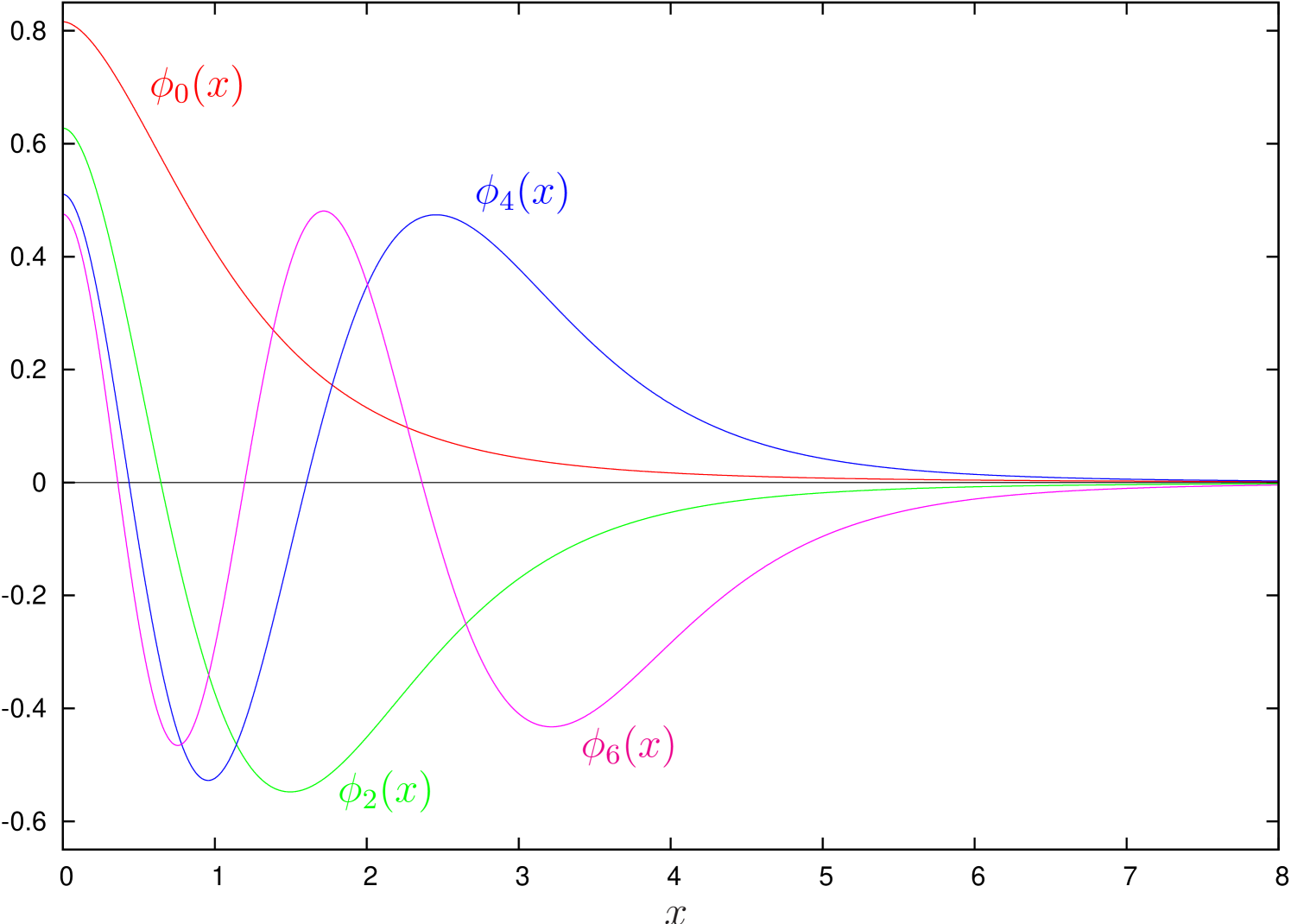
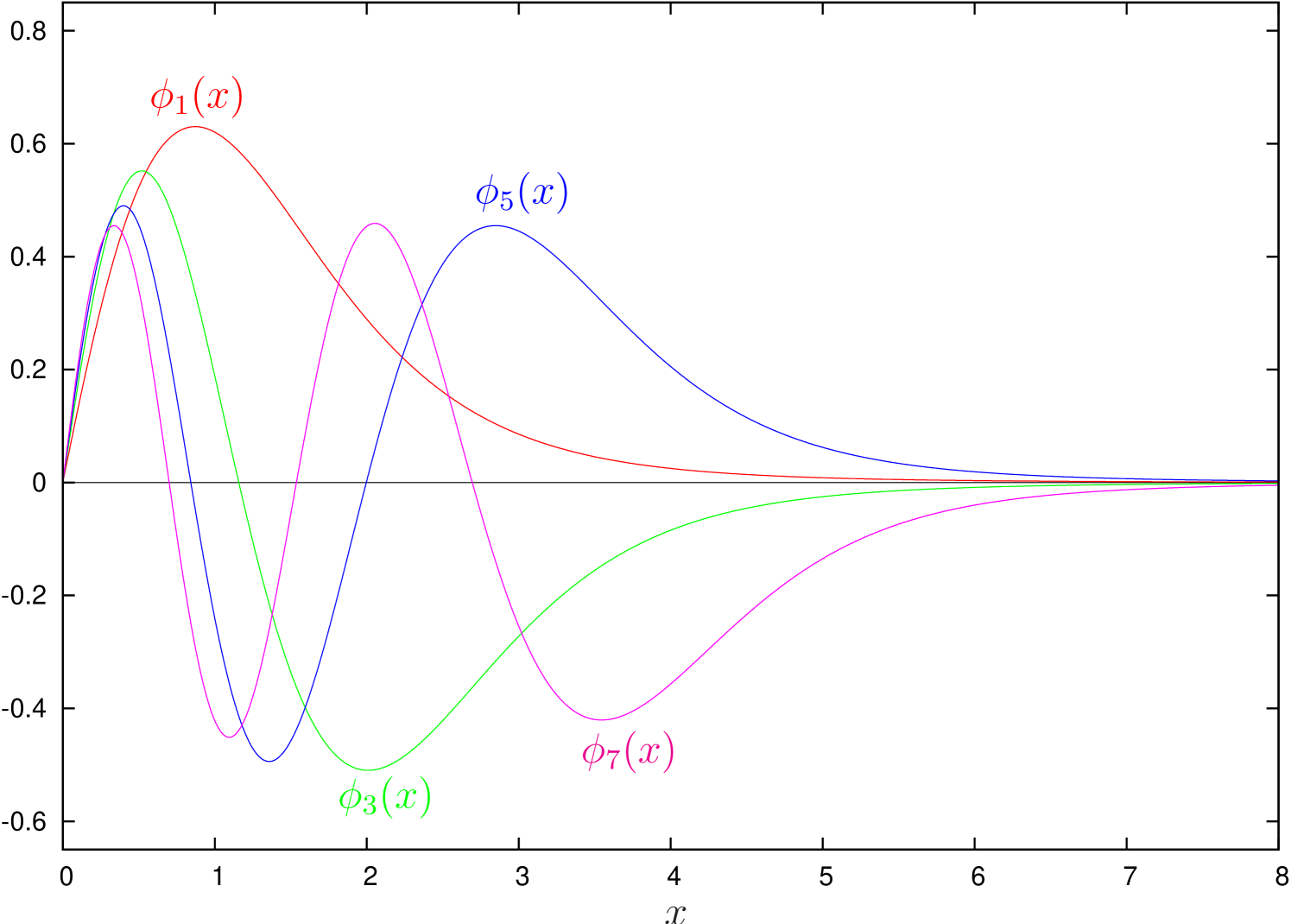
of (1). The results for , are listed in Table 1 and Figures 1 and 2. (We have chosen an odd number for , because this means that the position , where the potential is not differentiable, coincides with a lattice point. Including this point improves the convergence of the eigenvalues and functions for even.) From Table 1, we see that the quasi-classically obtained eigenvalues converge towards the numerically obtained values as is increased.
| 0 | 1.1849 | 0.57196 | 0.4681 | |
|---|---|---|---|---|
| 1 | 1.7443 | 0.96843 | 1.9494 | |
| 2 | 1.9517 | 0.94194 | 2.2398 | 0.64431 |
| 3 | 2.2842 | 1.17617 | 2.9428 | 1.15453 |
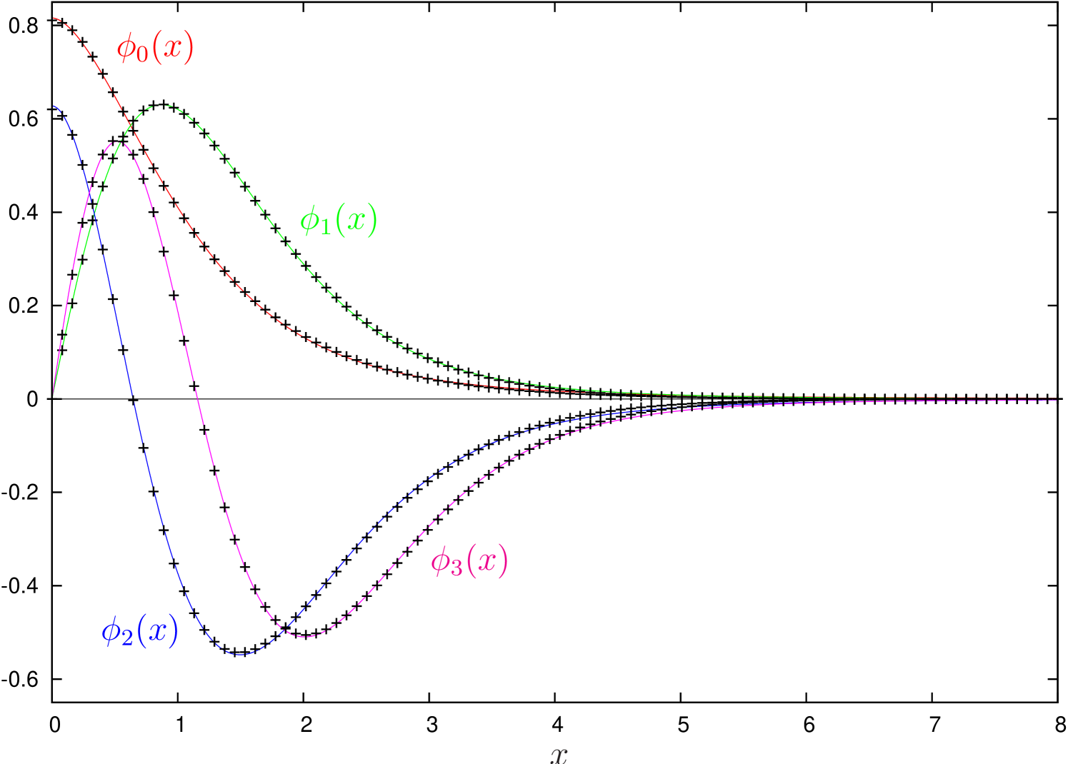
The eigenfunctions obtained numerically can be approximated by
| (22) |
for and by
| (23) |
for , with parameters , , , and listed in Table 2. Comparisons of these fits to the numerically obtained eigenfunctions are shown in Figure 3. The fits are not as good an approximation as Figure 3 may suggest, however, as they fall off as while the true eigenfunctions fall off as for even and as for odd as .
This asymptotic behavior of the eigenfunctions can be understood physically through second order perturbation theory. If we consider a small region around a point (i.e., very far away from the classically allowed region for the eigenstate with energy ), the amplitude there will be governed by scattering into this region from the classically allowed region, which contains almost the entire amplitude of the state. From (20), this scattering is proportional to
| (24) |
where is a cutoff to insure that we include the tail immediately surrounding the classically allowed region in the integral (from Figs. 1 and 2, we see that would be a reasonable choice). With the potential energy in the region we consider given by , the amplitude for finding the particle there will be proportional to for even and as for odd.
The numerical work reported here indicates that, within the limits of accuracy, the solutions are differentiable at , i.e., the expansion of around does not contain a term proportional to for even or for odd. Unfortunately, we have not been able to reach a conclusion regarding higher terms, and cannot tell whether there are terms proportional to for even or for odd.
V Further Considerations
It would be highly desirable to identify the exact eigenvalues and functions of (5). Unfortunately, we have as of yet not even succeeded in obtaining those for the ground state. A few thoughts on this problem, however, are possibly worth mentioning.
V.1 Fourier Symmetry
As the Hamiltonian (5) maps onto itself under Fourier transformation, and all the eigenstates are non-degenerate, the eigenfunctions must likewise map into itself under Fourier transformation (7),
| (25) |
This condition is directly fulfilled by certain functions, like the Gaussian eigenfunctions of the harmonic oscillator ,
or the function
The eigenfunctions of (5), however, do not need to be of any such particular form. For example, the Ansatz
| (26) |
It is conceivable that the function displays the required asymptotic behavior mentioned above, while the Fourier transform falls off more rapidly. A first guess for the ground state along these lines might be
| (27) |
with its Fourier transform given by a modified Bessel function of the second kind,
| (28) |
With , this provides a very reasonable approximation, but does not solve the problem exactly.
V.2 Asymptotic Behavior
V.3 Integral relations
We can apply some general properties of Hilbert transformations, defined asErdeyli54
| (37) |
where denotes the principle part, to rewrite (11). With
| (38) | |||||
| (39) |
we obtain
| (40) |
VI Conclusion
We have succeeded in solving the bi-linear oscillator both quasi-classically and numerically. In an attempt to solve it analytically as well, we have derived a differential and integral equation, and obtained the asymptotic behavior for large . We further formulated several conditions the solutions must satisfy. The problem of obtaining an analytical solution, however, is still open.
Acknowledgements.
I am grateful to R. von Baltz, W. Lang, A.D. Mirlin, and P. Wölfle for valuable discussions of this problem.References
- (1) B. Lake, A. M. Tsvelik, S. Notbohm, D. A. Tennant, T. G. Perring, M. Reehuis, C. Sekar, G. Krabbes, and B. Büchner, Nat. Phys. 6, 50 (2009).
- (2) M. Greiter, Nat. Phys. 6, 5 (2009).
- (3) T. Giamarchi, Quantum Physics in One Dimension (Oxford University Press, Oxford, 2004).
- (4) E. Dagotto and T. M. Rice, Science 271, 618 (1996).
- (5) D. G. Shelton, A. A. Nersesyan, and A. M. Tsvelik, Phys. Rev. B 53, 8521 (1996).
- (6) M. Greiter, Phys. Rev. B 66, 054505 (2002).
- (7) L. D. Landau and E. M. Lifshitz, Quantum Mechanics (Butterworth-Heinemann, Oxford, 1981).
- (8) Tables of Integral Transforms, edited by A. Erdélyi (McGraw-Hill, New York, 1954), Vol. II.