On the Lipschitz Saturation of Toric Singularities
Abstract
We begin the study of Lipschitz saturation for germs of toric singularities. By looking at their associated analytic algebras, we prove that if is a germ of toric singularity with smooth normalization then its Lipschitz saturation is again toric. Finally we show how to calculate the Lipschitz saturation for some families of toric singularities starting from the semigroup that defines them.
Introduction
For a germ of reduced complex analytic singularity, the algebra of germs of Lipschitz meromorphic functions is an analytic algebra that sits between and its normalization . The definition is algebraic, and was inspired by Zariski’s theory of saturation, whose objective was to establish the foundations for an algebraic theory of equisingularity as seen in [27], [28], [29] and [30]. It was first studied by Pham and Teissier in [21], where they prove that Lipschitz saturation and Zariski saturation coincide for hypersurfaces. In this paper they also introduced a relative notion of Lipschitz saturation whose algebraic treatment was further studied in [4], [5], [18]. Beyond the algebraic relevance of the construction, the associated germ is important in the study of biLipschitz equisingularity. The case of curves is pretty well understood and described in [6], [9], [12], [13], [20], [21]. However not much is known in higher dimensions. In this work we begin the study of the Lipschitz saturation for toric singularities of arbitrary dimension.
Our study is inspired by the fact that the Lipschitz saturation of a germ of irreducible curve is a toric curve, i.e., is parametrized by monomials. Moreover, there exists an explicit procedure for calculating its corresponding numerical semigroup starting from the semigroup of the curve. Although there is no reason to believe that the Lipschitz saturation of a germ of arbitrary dimension has toric structure, we may still ask the following question: starting with a toric singularity, is the Lipschitz saturation also toric? If so, is there a procedure for computing the corresponding affine semigroup from the semigroup of the toric singularity?
We answer the first question in the situation that naturally generalizes the case of toric curves, that is, toric varieties having smooth normalization. Regarding the question of the description of the corresponding semigroup, we provide an answer for some families of toric singularities.
An interesting semigroup theory aspect still lingers. The numerical semigroup of the Lipschitz saturation of a germ of toric curve can be calculated via the semigroup theoretic saturation as described in [22]. One can ask: if we start with a toric germ , is there an analogous operation on affine semigroups that calculates the affine semigroup of ? We conclude the paper by exhibiting examples showing that some properties of Lipschitz saturation of curves are no longer true in higher dimension. For instance, the embedding dimension has a different behavior.
The paper is divided as follows. In section 1 we recall the general construction of Lipschitz saturation and its main properties. We also recall some known facts in the case of curves. Furthermore, we prove that if a germ can be seen as the generic linear projection of another germ , then their Lipschitz saturations are isomorphic (proposition 1.4). This proposition has important consequences, for instance, it allows us to build examples of singularities that are not isomorphic to with toric Lipschitz saturation isomorphic to and toric normalization isomorphic to .
In section 2 we establish what we mean by a toric singularity , which is basically taking the germ at the origin of an affine toric variety. We summarize some important facts about the passage from the algebraic toric variety to the germ of analytic space. The results of this section are essentially known (see, for instance, [15]). We include them here for the sake of completeness.
In section 3 we prove our first main theorem: the Lipschitz saturation of a toric singularity whose normalization is smooth is again toric (theorem 3.2). The key idea towards this result is that for every all of its monomials are also in . We believe this result is true for toric singularities in general. However, the smooth normalization hypothesis is there for technical reasons (remark 3.4). As a first application, we show that the Whitney Umbrella singularity is Lipschitz saturated (see example 3.6).
In section 4 we use the tools previously developed to give a combinatorial description of the Lipschitz saturation for some families of toric singularities. More concretely, given the semigroup corresponding to the toric singularity , we explicitly describe the semigroup of its Lipschitz saturation (see proposition 4.1 and theorem 4.5). As a byproduct we can compute the embedding dimension of in these cases (see corollaries 4.2 and 4.6). We conclude by illustrating all these results in several examples.
1 Lipschitz saturation of complex analytic germs
The definition of Lipschitz saturation of a reduced complex analytic algebra is based on the concept of integral dependence on an ideal. Given an element and an ideal in a ring , we say that is integral over if satisfies a relation of the form
for some integer , with for . The set consisting of those elements of which are integral over is an ideal
called the integral closure of in (see [16], [19]).
Let us assume for simplicity that is irreducible and let be the integral closure of in its field of fractions. Geometrically, this corresponds to the normalization map and if we consider the holomorphic map
we get a surjective map of analytic algebras
where denotes the analytic tensor product which is the operation on the analytic algebras that corresponds to the fibre product of analytic spaces (for more details see [2] and [13]).
Definition 1.1.
Let be the kernel of the morphism above. We define the Lipschitz saturation of as the algebra
Remark 1.2.
A detailed discussion of the following facts can be found in [21, 13, 23]:
-
1.
is an analytic algebra and coincides with the ring of germs of meromorphic functions on which are locally Lipschitz with respect to the ambient metric.
-
2.
We have injective ring morphisms
-
3.
The corresponding Lipschitz saturation map
is a biLipschitz homeomorphism, induces an isomorphism outside the non-normal locus of and preserves the multiplicity, i.e.
Moreover, it can be realized as a generic linear projection in the sense of [13, Def. 8.4.2].
-
4.
and the holomorphic map induced by ,
is the normalization map of . Moreover the map
is the normalization map of .
Aside from these facts, little else is known in the general case. However, in the case of curves, the saturation has some very interesting equisingularity properties.
First, Pham and Teissier proved that for a plane curve the Lipschitz saturation determines and is determined by the characteristic
exponents of its branches and their intersection multiplicities, in particular the curve is an invariant of the equisingularity class of (See [21]
and [6, Prop. VI.3.2]).
In the irreducible case (branches) they also prove that the the curve is always a toric curve, (i.e parametrized by monomials), and if we have a parametrization of
then there is a simple procedure to calculate a parametrization of .
-
1.
Calculate the set of characteristic exponents of .
-
2.
Calculate the smallest saturated numerical semigroup containing as follows [22, Chapter 3, Section 2]:
-
3.
If is the minimal system of generators of then
is a parametrization of . Recall that in this setting is the multiplicity of and so we get that the embedding dimension of is equal to the multiplicity of .
These results extend well beyond the plane curve case: in [6, Thm VI.0.2, Prop. VI.3.1] the authors prove that for a curve , and a generic lineal projection the Lipschitz saturations of and of the plane curve are isomorphic. Even more, by [12, Thm. 4.12] we get that two germs of curves and are bi-Lipschitz equivalent if and only if their Lipschitz saturations are isomorphic. In this sense the saturated curve can be seen as a canonical representative of the bi-Lipschitz equivalence class of .
Example 1.3.
Let be the space curve with normalization map
For this curve, the projection on the first two coordinates is generic, giving us the plane curve
with characteristic exponents .
Following the procedure described above, we get the saturated numerical semigroup with minimal system of generators . This determines a parametrization of the saturated curve of the form:
Going back to the general case, we can prove that, just as in the case of curves, the Lipschitz saturation remains unchanged under generic linear projections.
Proposition 1.4.
Let be a germ of reduced and irreducible singularity, and let be a generic linear projection with respect to . Then and its image germ have isomorphic Lipschitz saturations, i.e.:
Before going through the proof, recall that the cone , constructed by taking limits of bi-secants to at , is an algebraic cone defined by H. Whitney in [25]. A linear projection with kernel is called -general (or generic) with respect to if it is transversal to the cone , meaning . When is generic, it induces a homeomorphism between and its image , and these two germs have the same multiplicity, for a detailed explanation see [13, Section 8.4].
Proof.
(of proposition 1.4)
After a linear change of coordinates we can assume that the linear projection is the projection on the first coordinates . Let denote the ideal defining the diagonal of
Denote . Then by [13, Proposition 8.5.11] the genericity of is equivalent to the equality of integral closures in .
On the other hand, since is a finite, generically 1-1 and surjective map, then the morphism
is injective, makes a finitely generated -module and induces an isomorphism of the corresponding field of fractions . All these together imply that and have isomorphic integral closures in and so if denotes the normalization of then the composition
is a normalization of .
Note that the ideal of definition 1.1 is defined by the “coordinate functions” of the normalization map
that is (see [13, Section 8.5.2]),
To prove the desired result it is enough to prove the equality of the integral closures . But the germ map:
induces a morphism of analytic algebras:
such that:
and since in the result follows. ∎
Note that in the course of the proof we have shown that the germ and its general projection have isomorphic normalizations. On the downside, it will no longer be true in general that bi-Lipschitz equivalent germs will have isomorphic Lipschitz saturations. This is because a germ and its Lipschitz saturation always have the same multiplicity, however in [3] the authors prove that in dimension bigger than two, multiplicity of singularities is not a bi-Lipschitz invariant.
2 Toric singularities
In this section we establish what we mean by a toric singularity. We also introduce the notation we use regarding toric varieties.
Let , , and . Assume that the group generated by is and that is a strongly convex cone. Consider the following homomorphism of semigroups,
and the induced algebra homomorphism,
Let . Recall that is a prime ideal and Let be the affine variety defined by . Then is a -dimensional affine toric variety containing the origin. Let be the ring of regular functions on and the -algebra of the semigroup . Recall that [7, Chapter 1].
Next we discuss some basic results on the passage from the algebraic toric variety to the germ of analytic space . Throughout this section we use the following notation.
-
•
denotes the ring of formal power series with exponents in .
-
•
denotes the subring of consisting of convergent series in a neighborhood of .
-
•
denotes the algebra of germs of holomorphic functions on .
Remark 2.1.
Notice that is indeed a ring since is contained in a strongly convex cone which implies that every element of can be written as a sum of elements of in finitely many different ways.
Lemma 2.2.
With the previous notation,
Proof.
The first isomorphism is proved in [15, Lemme 1] or [14, Lemma 1.1]. The proof given there is for normal toric varieties. However, the same proof holds in the non-normal case.
We prove the second isomorphism. Consider the following exact sequence:
Let . Taking completions with respect to we obtain the following exact sequence:
On the other hand, [1, Proposition 10.15]. Denote . In the proof of [14, Lemma 1.1], alternatively [15, Lemme 1] it is shown that . It remains to prove that .
Since , it follows that . Let be such that . We conclude that (these ideals are equal by [8, Exercise 8.1.5]). ∎
Lemma 2.3.
Let be the (algebraic) normalization of . Then is the (analytic) normalization of . Moreover,
Proof.
Let be the normalization. Recall that is the toric variety defined by the semigroup and that is induced by the inclusion of semigroups [7, Proposition 1.3.8]. In particular, is a toric morphism.
Being the normalization, is an isomorphism on dense open sets. In addition, . Indeed, let be such that . Recall that points in toric varieties correspond to homomorphisms of semigroups. Hence, the homomorphism corresponding to sends every non-zero element of to 0. On the other hand, for every there is such that . Since is induced by the inclusion , it follows that .
By the previous paragraph, the induced germ of an analytic function is finite and generically 1-1. On the other hand, it is known that normal implies that normal [17, Satz 4]. By the uniqueness of normalization we conclude that is the normalization of .
Finally, follows using lemma 2.2. ∎
Corollary 2.4.
is irreducible as a germ.
Proof.
Definition 2.5.
Let be a germ of an analytic space. We say that is a germ of a toric singularity if there exists a finitely generated semigroup contained in a strongly convex cone such that . Equivalently, let be the affine toric variety defined by . Then is a toric singularity if it is isomorphic, as germs, to .
Example 2.6.
Let be a toric variety containing the origin. Then is a germ of a toric singularity by lemma 2.2.
3 Lipschitz saturation of toric singularities
We have seen that for a toric singularity the analytic algebra is generated by monomials. With this in mind, the main idea to prove that the Lipschitz saturation of a toric singularity is again toric, consists of showing that every monomial of an element of the saturation also belongs to the saturation. The first step towards that goal is the study of the integral closure of homogeneous ideals in the ring of power series.
It is well known that the integral closure of a homogeneous ideal in a polynomial ring is again a homogeneous ideal ([24, Prop. (f), pg 38]). However we need this to be true for ideals generated by homogeneous polynomials in power series rings. That is the content of the following proposition, whose proof was kindly communicated to us by Professors Irena Swanson and Craig Huneke.
Note that an ideal is generated by homogeneous polynomials if and only if implies that every homogeneous component of is also in .
Proposition 3.1.
Let be an ideal generated by homogeneous polynomials in the ring of convergent power series. Then its integral closure is also generated by homogeneous polynomials.
Proof.
Let denote the ring of convergent power series in -variables over the field of complex numbers with maximal
ideal , and let where each is a homogeneous polynomial.
Let be the ideal generated by the ’s in the polynomial ring , so . Suppose that contains a power of , i.e. there exists such that , and let be in the integral closure of . We can write
where is a polynomial and is a series of order greater than or equal to . Note that .
Since the ring extension is faithfully flat ([11, Lemma B.3.4]) then ([16, Prop.1.6.2]), in particular . This means that in the localized polynomial ring we have an equation of integral dependence of the form:
where and . Letting and multiplying this equation by the unit of we get the following equality in :
Since A is an integral domain we get an integral dependence equation in
that is, . The inclusions imply that is an -primary ideal of and since then . Since is a homogeneous ideal in the polynomial ring then is also homogeneous ([24, Prop. (f), pg 38]) and so each homogeneous component of is also in . This implies that is also generated by homogeneous polynomials.
Now let be an arbitrary ideal generated by homogeneous polynomials, and let be in the integral closure as before. Let be the initial form of , is the non-zero homogeneous component of of lowest degree. For all , is in the integral closure of . We proved in the previous paragraph that the integral closure of in is generated by homogeneous polynomials for all . In particular, is in the integral closure for all . But by [16, Corollary 6.8.5] this implies that is in the integral closure . Now we start over with and in this way we get that all homogeneous components of are in which is what we wanted to prove. ∎
Theorem 3.2.
Let be a -dimensional toric singularity with smooth normalization. Then the Lipschitz saturated germ is also a toric singularity.
We will do this proof in several steps starting with the following lemma.
Lemma 3.3.
Let be a -dimensional toric singularity with smooth normalization and let be a homogeneous polynomial such that . Then every monomial of is also in .
Proof.
Let be the semigroup defining . Recall that is a strongly convex cone. This fact, together with the condition of smooth normalization allows us to assume, up to a change of coordinates, that and (see lemma 2.3).
Let be the minimal generating set of defining the toric singularity . The normalization map can be realized as the monomial morphism:
The ideal of definition 1.1 is a homogeneous, binomial ideal in the ring of convergent power series :
For any point we have an automorphism
defined by and , such that .
Now let be a homogeneous polynomial such that . Then and it satisfies an integral dependence equation of the form:
where . By applying the morphism to the previous equation we get:
where , and so we get that .
Since is a homogeneous polynomial, say of order , then we can write it in the form
where and . Then we have an expression for of the form
By choosing generic points in we get
where the -th row of the matrix corresponds to the image of the point of the Veronese map of degree . Since the image of the Veronese map is a nondegenerate projective variety, in the sense that it is not contained in any hyperplane, then these points are in general position. This implies that the matrix is invertible, and so we have
In particular we have that which is what we wanted to prove. ∎
Proof.
(of theorem 3.2 )
We want to prove that there exists a finitely generated semigroup such that
As we mentioned before, in this setting the ideal is a homogeneous, binomial ideal in the ring of convergent power series , and by proposition 3.1 the ideal is also generated by homogeneous polynomials. This means that if a series is in ,
then every homogeneous component of is in . But by lemma 3.3 this implies that every monomial of degree with a non-zero coefficient in is also in . Let be the semigroup defined by
We have that
We have to prove that is finitely generated and the equality .
To begin with the latter, take . For every , write where is the truncation of to degree , and since it is a finite sum of monomials of , by definition of , we have that . This means that
and since we have that
In particular,
then and we have the equality we wanted.
Now we prove that is a finitely generated semigroup. Let be a monomial order in . We order the elements of and write them as , where . Consider the following ascending chain of ideals in :
Since is Noetherian, we have , for some and for all . We claim that .
Indeed, let , for some . Since it follows that , for some and some monomial of . As before, we have . Hence, is the sum of plus an element and . Continuing this way, we obtain that . ∎
Remark 3.4.
We now know that for a germ of toric singularity with smooth normalization and associated semigroup , the Lipschitz saturated germ is again a toric singularity with associated semigroup . In this setting we have and we need to determine which elements we have to add to in order to obtain . Since many properties of a toric variety are encoded in its semigroup, we can use them to start discerning. This is the content of the following proposition.
Proposition 3.5.
Let be a germ of -dimensional toric singularity with smooth normalization. Let be the associated semigroup and the convex hull of in . If then .
Proof.
In the case of curves, this means that if is the minimal non-zero element of then , with implies that (see section 1). Recall that in this case is equal to the multiplicity of the curve.
Example 3.6.
The Whitney Umbrella.
The surface singularity defined by the equation is a toric singularity with smooth normalization
given by
and associated semigroup with minimal generating set . This translates to and a point is identified with the monomial .
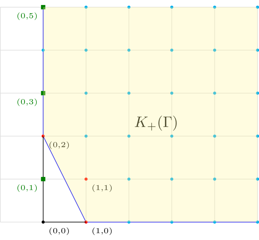
Note that . We will show that none of them are in . Hence, . In the proof of theorem 3.2 we showed that . We conclude that and so the Whitney Umbrella coincides with its Lipschitz saturation .
To begin with, the only point in is , and so by the previous proposition. For the points of the form with odd, consider the ideal
Taking the arc defined by we have the corresponding morphism of analytic algebras such that
By [19, Thm 2.1] this implies that , i.e. .
4 Some examples.
In this section we will show how to calculate the Lipschitz saturation of some families of toric singularities, starting with products of curves.
Let and be two germs of toric singularities of dimension defined by the semigroups and with corresponding minimal generating sets and . The germ is a toric surface singularity with semigroup generated by , that is . Note that the normalization of is smooth and the normalization map can be written as
Proposition 4.1.
For a germ of surface singularity defined by a product of toric curves, the Lipschitz saturation is a toric surface singularity with semigroup
where and are the semigroups of the Lipschitz saturated curves and described in section 1.
Proof.
We know that is an analytic algebra generated by monomials, so we need to characterize them. A monomial defines a meromorphic function on a neighborhood of the origin in which is locally Lipschitz with respect to the ambient metric. If we consider the normalization of as before
then for any sufficiently small the restriction of to tells us that defines a meromorphic locally Lipschitz function on and so ; equivalently . The same reasoning with the restriction to tells us that and so .
On the other hand, in this setting we have the ideal defined by
Let then by definition we have
In particular, and so . Analogously for every we have . Since is an analytic algebra, this implies that for every and the monomial which finishes the proof. ∎
Corollary 4.2.
Let be a product of toric curves. Then . In addition, .
Proof.
First, recall that the embedding dimension of the origin of a toric variety i.e., the dimension of its Zariski tangent space, coincides with the cardinality of the minimal generating set of the correspondig semigroup. On the other hand, the multiplicity at the origin of a toric variety is also described combinatorially in terms of the semigroup (see proposition 3.5). Hence, both assertions follow from proposition 4.1. ∎
Remark 4.3.
Example 4.4.
Starting from the space curves and parametrized respectively by
we get the toric surface of multiplicity and embedding dimension defined by the ideal
The normalization map is given by:
Following the procedure described in section 1 we obtain that the semigroup is generated by and the semigroup is generated by . By proposition 4.1 the Lipschitz saturation is the toric singularity defined by the semigroup generated by the set
and with normalization map given by:
is a toric germ of multiplicity and embedding dimension .
Since is a germ of singular surface, we have that the cone is of dimension or and so almost every linear projection
is generic, in the sense that it is transversal to this cone (see [13, Prop. 8.4.3]). Using proposition 1.4, for each such we get a germ of singular surface of multiplicity and embedding dimension at most , with normalization map (see the proof of proposition 1.4)
This gives us a family of surfaces that are not isomorphic to whose Lipschitz saturation is toric and isomorphic to .
We will now a consider a family of hypersurfaces with equation of the form
where and . It is a family of toric surface singularities with semigroup generated by .
Theorem 4.5.
Let be the toric hypersurface singularity with normalization map given by
where and . Let be the numerical semigroup generated by , and be its saturation as in section 1. The monomial is in the Lipschitz saturation if and only if for some or and .
Proof.
In this setting the semigroup is generated by , and by the proof of theorem 3.2
is equivalent to .
We first show that if for some or and then . Suppose first that . Since , it follows that for all .
Now suppose that and . Since we have that and so it is enough to prove the statement for . By definition if and only if where
The assumption means that , which can be rephrased in terms of integral closure of ideals by
And so if we denote by we have an integral dependence equation in of the form:
with . Each will then be of the form
Multiplying the integral dependence equation by we obtain:
| (1) |
But now
Note that implies that . In particular we get
and so . This implies that equation (1) is an integral dependence equation for
over . Finally and
imply which is what we wanted to prove.
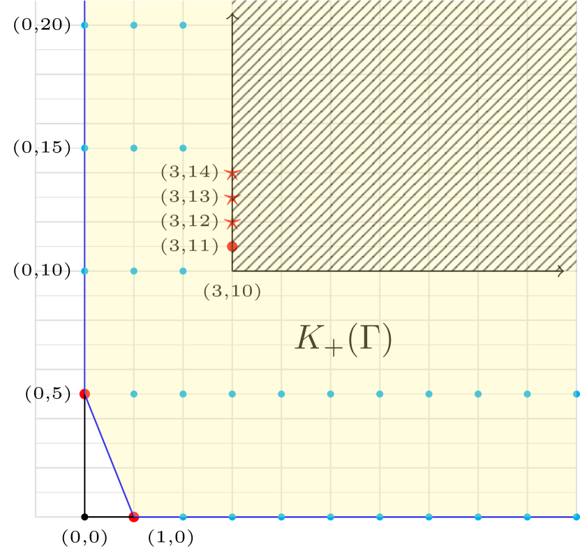
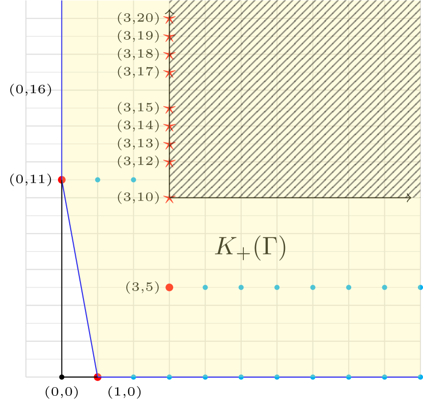
Now we prove that implies for some or and .
If for some , we are done. Assume that for all . We show that and .
Note that for any we have an embedding of the plane toric curve , with semigroup generated by and defined by , via the map
By remark 1.2 a monomial defines a locally Lipschitz meromorphic function on a small enough neighborhood of in . For any small enough it restricts to a locally Lipschitz meromorphic function on a neighborhood of in the embedded curve . In particular , or equivalently .
To show that we prove that and implies . We consider two cases: and .
Following example 3.6, note that all points of the form with are in and so they are not in by proposition 3.5. For the points of the form with , , consider the ideal
Let be a primitive -th root of unity and consider the arc
We have the corresponding morphism of analytic algebras such that
In particular,
By [19, Thm 2.1] this impliest that , i.e. .
All that is left to prove is that for and the monomial is not in . We will once again use the arc criterion for integral dependence, but this time with the arc
where is a primitive -th root of unity. In this setting the image of by the morphism in is of the form:
On the other hand we have
Using that it is straightforward to verify that for every
and so , i.e. .
∎
Corollary 4.6.
Let be a germ of toric hypersurface singularity as in theorem 4.5. Then is a toric surface singularity of multiplicity and embedding dimension .
Proof.
By the combinatorial description of multiplicity in toric geometry, it follows that . Similarly, the embedding dimension of corresponds to the cardinality of the minimal set of generators of . We exhibit this minimal set of generators and show that it has cardinality .
Theorem 4.5 states that if and only if for some or and . We divide the proof in two cases.
Case . Write , and . By the algorithm for computing we obtain (see section 1). Consider the sets
We claim that . Firstly observe that . Now let . If then . In particular, this holds for the element . Now assume that and . Since it is enough to consider .
-
•
Suppose . Then for some . Hence .
-
•
Suppose . Then .
-
•
Suppose , . Then .
-
•
Suppose . Write , , . Then .
Now we show that is minimal as a generating set. Indeed, first notice that no element of can be generated by and viceversa (because of the second entry of the vectors). Similarly, for each it follows that (because of the first entry of the vectors). Hence is the minimal generating set of and has cardinality .
Case . Write , and . We compute as before: . Consider the sets
We claim that . Firstly observe that . Now let . If then . Now assume that and . As before, it is enough to consider .
-
•
For each we have .
-
•
Suppose . Then for some . Hence .
-
•
Suppose . Then .
-
•
Suppose , , . Then .
-
•
Suppose . Write , , . Then .
A similar analysis as in the previous case shows that is the minimal generating set of and has cardinality . ∎
Example 4.7.
Consider the toric hypersurface singularity with normalization map
It is defined by the equation and so it has multiplicity . Following the notation of theorem 4.5 we have the semigroup generated by and its saturation with minimal generating set .
From the previous corollary we have the semigroup associated to the Lipschitz saturation with minimal generating set
normalization map
and embedding dimension .
Interchanging the roles of and we get the following example.
Example 4.8.
Consider the toric hypersurface singularity with normalization map
It is defined by the equation and so it has multiplicity . Following the notation of theorem 4.5 we have again the semigroup generated by and its saturation with minimal generating set .
From the previous corollary we have the semigroup associated to the Lipschitz saturation with minimal generating set
normalization map
and embedding dimension .
Note that in both examples we have .
Remark 4.9.
Recall from section 1 that the Lipschitz saturation of an irreducible curve has multiplicity equal to its embedding dimension. The results and examples from this section shows that there is no general relation among the embedding dimension and the multiplicity of the Lipschitz saturation in higher dimensions.
Remark 4.10.
Contrary to the case of curves, for the moment it is not clear that there exists an explicit algorithm to compute the semigroup from the semigroup , in general. We proved in theorem 3.2 that is finitely generated by Noetherian arguments, hence we do not have a constructive procedure to obtain a set of generators. However, the same theorem shows that the toric structure is preserved under Lipschitz saturation so, in principle, there should be a semigroup operation that provides . It remains an open question to find an algorithm that produces generators for in general.
Acknowledgements
The authors would like to thank professors P. Gonzalez Perez, C. Huneke and I. Swanson for the fruitful e-mail exchanges that greatly helped in the preparation of this work. They also acknowledge support by PAPIIT grant IN117523 and CONAHCYT grant CF-2023-G-33. A. Giles Flores acknowledges support by UAA grants PIM21-1 and PIM24-7.
References
- [1] Atiyah, M. F., Macdonald, I. G.; Introduction to Commutative Algebra, Addison-Wesly, 1969.
- [2] J. Adamus, in Topics in Complex Analytic Geometry Part II. Lecture notes https://www.uwo.ca/math/faculty/adamus/adamus_publications/AGII.pdf
- [3] L. Birbrair, A. Fernandes, J.E. Sampaio, M. Verbitsky; Multiplicity of singularities is not a bi-Lipschitz invariant, in Mathematische Annalen 377, pp. 115-121, Springer 2020.
- [4] E. Böger; Zur Theorie des Saturation bei analytischen Algebren, Math. Ann. 211 (1974), pp. 119-143.
- [5] E. Böger; Über die Gleicheit von absoluter und relativer Lipschitz Saturation bei analytischen Algebren, Manuscripta Math. 16 (1975), pp. 229-249.
- [6] J. Briancon, A. Galligo, M. Granger; Déformations équisinguliéres des germes de courbes gauches réduites. Mém. Soc. Math. France, 2éme serie (1), 69, 1980.
- [7] D. Cox, J. Little, H. Schenck; Toric Varieties, Graduate Studies in Mathematics, Vol. 124, AMS, 2011.
- [8] de Jong, T., Pfister, G.; Local Analytic Geometry, Vieweg, 2000.
- [9] A. Fernandes; Topological equivalence of complex curves and bi-Lipschitz maps, Michigan Math. J, Vol 51, pp 593-606, 2003.
- [10] I.M. Gelfand, M.M. Kapranov, A.V. Zelevinsky; Discriminants, Resultants and Multidimensional Determinants, Modern Birkhäuser Classics, 2008.
- [11] G.M. Greuel, C. Lossen, E. Shustin; Introduction to Singularities and Deformations, Springer Monographs in Mathematics, 2007.
- [12] A. Giles Flores, O.N. Silva, J. Snoussi; On the fifth Whitney cone of a complex analytic curve, Journal of Singularities, vol 24, pp. 96-118, 2022.
- [13] A. Giles Flores, O.N. Silva, B. Teissier; The biLipschitz Geometry of Complex Curves: an algebraic approach, in Introduction to Lipschitz Geometry of Singularities, ed. by W. Neumann, A. Pichon. Lecture Notes in Mathematics, vol 2280, pp 217-271, Springer International Publishing, 2020.
- [14] P. D. González Perez; Quasi-ordinary singularities via toric geometry, Ph. D. Thesis, Universidad de la Laguna, 2000.
- [15] P. D. González Perez; Singularités quasi-ordinaires toriques et polyèdre de Newton du discriminant., in Canadian Journal of Mathematics, 52(2), 348-368. doi:10.4153/CJM-2000-016-8
- [16] C. Huneke, I. Swanson, Integral Closure of Ideals, Rings and Modules, London Mathematical Society Lecture Note Series, no 336, Cambridge University Press, 2006.
- [17] N. Kuhlmann; Die Normalisierung komplexer Räume, Math. Ann. 144 (1961), pp 110-125.
- [18] J. Lipman; Relative Lipschitz saturation, Am. J. Math 98-2 (1975), pp 791-813.
- [19] M. Lejeune-Jalabert, B. Teissier; Clôture intégrale des idéaux et equisingularité, Ann. Fac. Sci. Tolouse Math. (6) 4, 781-859, 2008.
- [20] W.D. Neumann, A. Pichon; Lipschitz Geometry of Complex Curves, Journal of Singularities, vol 10, pp 225-234, 2014.
- [21] F. Pham, B. Teissier; Lipschitz Fractions of a Complex Analytic Algebra and Zariski Saturation, in Introduction to Lipschitz Geometry of Singularities, ed. by W. Neumann, A. Pichon. Lecture Notes in Mathematics, vol 2280, pp 309-337, Springer International Publishing, 2020.
- [22] J.C. Rosales, P.A. García-Sánchez, Numerical Semigroups, Developments in Mathematics (Springer Berlin), 2009. American Mathematical Society, Providence, RI, 1996.
- [23] B.Teissier, Varétés polaires II: Multiplicités polaires, sections planes et conditions de Whitney, in Algebraic geometry, Proc. int. Conf., La Rábida/Spain 1981. Lecture Notes in Mathematics, vol. 961 (Springer Berlin, 1982), pp. 314-491.
- [24] W. Vasconcelos; Integral Closure: Rees algebras, multiplicities, algorithms, Springer Monographs in Mathematics, 2005.
- [25] H. Whitney, Local properties of analytic varieties, in Differ. and Combinat. Topology, Sympos. Marston Morse, Princeton 1965, pp. 205-244.
- [26] O. Zariski; Analytical irreducibility of normal varieties, Ann. of Math., Vol. 131, No. 2, (1948), pp 352-361.
- [27] O. Zariski; Studies in equisingularity III, Saturation of local rings and equisingularity, Am. J. Math. 90 (1968), pp 961-1023.
- [28] O. Zariski; General theory of saturation and of saturated local rings I, Am. J. Math. 93 (1971), pp. 573-648.
- [29] O. Zariski; General theory of saturation and of saturated local rings II, Am. J. Math. 93 (1971), pp. 872-964.
- [30] O. Zariski; General theory of saturation and of saturated local rings III, Am. J. Math. 97 (1975), pp. 415-502.
D. Duarte, Centro de Ciencias Matemáticas, UNAM.
E-mail: adduarte@matmor.unam.mx
A. Giles Flores, Universidad Autónoma de Aguascalientes.
Email: arturo.giles@edu.uaa.mx