On the Return Distributions of a Basket of Cryptocurrencies and Subsequent Implications
(First Draft: May 14, 2021)
Abstract
This paper evaluates and assesses the risk associated with capital allocation in cryptocurrencies (CCs). In this regard, we take a basket of 27 CCs and the CC index EWCI- into account. After considering a series of statistical tests we find the stable distribution (SDI) to be the most appropriate to model the body of CCs returns. However, as we find the SDI to possess less favorable properties in the tail area for high quantiles, the generalized Pareto distribution is adapted for a more precise risk assessment. We use a combination of both distributions to calculate the Value at Risk and the Conditional Value at Risk, indicating two subgroups of CCs with differing risk characteristics.
keywords:
Body-/Tail-Models , Cryptocurrencies , Index Construction , Market Segmentation , Statistical TestsJEL Classification: C12 , C13 , C43 , E22.
ORCID IDs: 0000-0001-5722-3086 (Christoph J. Börner), 0000-0001-7575-5537 (Ingo Hoffmann), 0000-0002-0978-6252 (Jonas Krettek), 0000-0001-5774-1983 (Lars M. Kürzinger), 0000-0001-9002-5129 (Tim Schmitz).
Acknowledgement: We thank Coinmarketcap.com for generously providing the cryptocurrency time series data for our research.
1 Introduction
Following the financial crisis of 2007 and a period of extreme uncertainty and volatility, trust in the financial system and its institutions, like central banks and their monetary policies, have been shattered (Kaya Soylu et al., 2020; Bouri et al., 2017a).
Against this background, the market for cryptocurrencies (CCs) started to emerge in 2009 with the development of the Bitcoin by Nakamoto (2008). This innovative peer-to-peer electronic cash system is not accountable to any subordinate institution, but is managed and controlled by its own community using the blockchain technology. Furthermore, the anonymity and security of transactions represent another noteworthy feature Bitcoin promises its users (Kakinaka and Umeno, 2020), resulting in increasing trading volumes and prices (Corbet et al., 2019). This development raises questions for both investors and regulators alike regarding the CC market’s characteristics and risk profile, which need to be answered in order for CCs to become an investable asset class for a broad audience (Gkillas and Katsiampa, 2018; Majoros and Zempléni, 2018; Osterrieder et al., 2017) and to provide guidance for risk management in general (Kakinaka and Umeno, 2020). In this regard, this study examines the question which class of distribution functions models CC returns most accurately. We answer this question using a novel approach to separate a distribution’s body from its tail proposed by Hoffmann and Börner (2021). By doing so we are able determine the risk and statistical properties associated with CCs and provide valuable implications for portfoliomanagement and regulators alike.
Even though the technical properties of CCs are well understood, CCs’ behavior remains to be fully comprehended and analyzed. As of today, many economic studies have focused on Bitcoin and other prominent CCs such as Ethereum and Ripple since they dominate the CC market due to their high proportion of total market capitalization (Glas, 2019). In this regard, Baur et al. (2018) and Glas (2019) find Bitcoin and other CCs to be uncorrelated to traditional assets in times of financial distress. Additionally, Gkillas et al. (2018), show CC’s behavior to differ from fiat currencies as well. Furthermore, various studies analyze certain characteristics of CCs like e.g. volatility (Polasik et al., 2015; Balcilar et al., 2017), diversification issues (see i.a. Brière et al. (2015); Selgin (2015); Corbet et al. (2018)) and safe haven properties (Bouri et al., 2017b; Urquhart, 2018)111For a more extensive literature review, see Corbet et al. (2019)..
However, in order to evaluate the corresponding market risk and to completely understand the CC market as a whole, we follow other studies in analyzing return distributions of the CC market. As numerous studies observe non gaussian behavior and heavy tails in return distributions (Osterrieder et al., 2017; Gkillas et al., 2018; Gkillas and Katsiampa, 2018), a distribution model accounting for these observed characteristics ought to be implemented. To account for these properties Majoros and Zempléni (2018) and Kakinaka and Umeno (2020) utilize the class of stable distributions (SDIs) in their recent studies. However, Kakinaka and Umeno (2020) observe the SDI to be unable to efficiently grasp the heavy tails of the analyzed return distributions in all scenarios in comparison to other possible distributions. Given this background, the generalized Pareto distribution (GPD), a statistical distribution which appears to model heavy tail properties more accurately, is used in further studies (Gkillas et al., 2018; Gkillas and Katsiampa, 2018). Following the approach presented in Hoffmann and Börner (2021), we therefore attempt to use a combination of both described distributions. Analytically discovering the beginning of the tail of the analyzed return distributions, enables us to split the given data into a body and a tail for each of which we implement a different distribution. For the first sample, containing the tail of potential losses, we implement the GPD, since literature and our conducted tests show its goodness of fit for estimating tail values. For the remaining body of our data we apply the SDI as its fit outperforms other possible distributions.
Our study aims to add to the existing literature by implementing a novel approach, which tries to reach a higher quality of modelling return distributions observed in the CC market. Furthermore, as of today most studies are merely concerned with analyzing characteristics of Bitcoin or the most prominent CCs like i.a. Ethereum, Ripple and Litecoin ((Baur et al., 2018; Bouri et al., 2017b; Osterrieder et al., 2017; Gkillas et al., 2018; Gkillas and Katsiampa, 2018; Majoros and Zempléni, 2018; Kakinaka and Umeno, 2020). Therefore, most studies do not consider the entirety of the CC market, which, as Glas (2019) points out, might lead to potential bias. Hence, we join Glas (2019) and ElBahrawy et al. (2017), in an attempt to give a broader overview of the CC market. By doing so we tackle two existing gaps in literature found by Corbet et al. (2019) in their extensive literature review. Namely, we extend the number and size of analyzed data in an attempt to analyze CCs as an asset class. Furthermore, our reserach does provide practical relevance in form of an improved risk assessment. By analytically separating a distribution’s body from its tail and implementing different distributions, we are able to estimate risk measures in form of the Value at Risk and the Conditional Value at Risk more precisely. Both of which do yield an importance for regulators and investors alike.
The remainder of this paper is structured as follows: In Sec. 2 we present and describe our data used for our following analysis. In Sec. 3 we perform a series of statistical analyses and tests which lead us to the family of SDIs as the best model choice for the body of the CCs returns distribution. Based on these findings, Sec. 4 is concerned with the assessment of the tail risk inherent in an investment in a single CC or the basket aggregated in the EWCI-. We compare both methods of the risk assessment at high quantiles. First we use the body model and second we adapt the GPD as tail model for risk assessment in terms of the Value at Risk and the Conditional Value at Risk. The last section summarizes our most import results and gives an overview of further research topics.
2 Data
As a foundation of our analysis, we follow various studies, by extracting CCs’ daily prices from the website coinmarketcap.com (i.a. (Fry and Cheah, 2016; Hayes, 2017; Brauneis and Mestel, 2018; Caporale et al., 2018; Gandal et al., 2018; Glas, 2019). For an observation period from 2014-01-01 to 2019-06-01, we take CCs from the Coinmarketcap Market Cap Ranking at the reference date of 2014-01-01 into consideration, cf. Tab. 1.
In order to depict the CC market as a whole, we aim to include as many CCs in our analysis as possible. However, as data gaps appear in the time series of most CCs considered, we exclude all CCs with five or more consecutive missing observations. By utilizing the Last Observation Carried Forward (LOCF) approach, as previously done in Schmitz and Hoffmann (2020) and Trimborn et al. (2020), we are able to include all CCs with smaller data gaps.
After taking these considerations into account, 27 CCs remain in our data set, all of which are depicted in bold letters in cf. Tab. 1. In a next step, we convert the CC prices denoted in USD to EUR prices, using the daily USD-EUR exchange rates retrieved from Thomson Reuters Eikon. For the purpose of preventing potential weekday biases, the resulting (daily) observations are converted to weekly observations in a following step. In a final step, we calculate logarithmic returns using these weekly CC EUR prices for each CC, which we will refer to as returns in the remainder of this paper.
| CC | ID | CC | ID | CC | ID |
|---|---|---|---|---|---|
| Anoncoin | ANC | Argentum | ARG | AsicCoin | ASC |
| BBQCoin | BQC | BetaCoin | BET | BitBar | BTB |
| Bitcoin | BTC | BitShares PTS | PTS | Bullion | CBX |
| ByteCoin | BTE | CasinoCoin | CSC | CatCoin | CAT |
| Copperlark | CLR | CraftCoin | CRC | Datacoin | DTC |
| Deutsche e-Mark | DEM | Devcoin | DVC | Diamond | DMD |
| Digitalcoin | DGC | Dogecoin | DOGE | Earthcoin | EAC |
| Elacoin | ELC | EZCoin | EZC | FastCoin | FST |
| Feathercoin | FTC | Fedoracoin | TIPS | FLO | FLO |
| Franko | FRK | Freicoin | FRC | Globalcoin | GLC |
| GoldCoin | GLC | GrandCoin | GDC | HoboNickels | HBN |
| I0Coin | I0C | Infinitecoin | IFC | Ixcoin | IXC |
| Joulecoin | XJO | Junkcoin | JKC | Litecoin | LTC |
| LottoCoin | LOT | Luckycoin | LKY | Megacoin | MEC |
| MemoryCoin | MMC | MinCoin | MNC | Namecoin | NMC |
| NetCoin | NET | Noirbits | NRB | Novacoin | NVC |
| Nxt | NXT | Omni | OMNI | Orbitcoin | ORB |
| Peercoin | PPC | Philosopher Stones | PHS | Phoenixcoin | PXC |
| Primecoin | XPM | Quark | QRK | Ripple | XRP |
| SexCoin | SXC | Spots | SPT | StableCoin | SBC |
| TagCoin | TAG | Terracoin | TRC | Tickets | TIX |
| TigerCoin | TGC | WorldCoin | WDC | Zetacoin | ZET |
For an aggregated perspective on CCs, we use the above-mentioned weekly CC data to calculate an Equally-Weighted CC Index (EWCI), as it is similarly done in Schmitz and Hoffmann (2020). Whereas, as we exclude more CCs in comparison to Schmitz and Hoffmann (2020), we will call this index EWCI- for a more precise distinction.
3 The return distribution of cryptocurrencies
For an initial classification of CCs simple statistical key figures from the standard repertoire of empirical statistics are used below. The description and evaluation of additional statistical properties of CCs, for example Value at Risk or lower-partial moments, are carried out using a suitable distribution function. Our results show that the family of SDIs is a suitable model for the examined returns of CCs. Hence, this family of distributions is used in Sec. 4 for a more in-depth analysis of the statistical properties of CCs.
3.1 Determination of basic statistical key figures of the cryptocurrencies
Standard procedures lead us to estimates of the set of basic statistical key figures: mean , variance and the bandwidth (Tab. 2.).
| Crypto | Mean | Variance | Bandwidth | HDS-Test | SIG-Test | |||
|---|---|---|---|---|---|---|---|---|
| ID | min | max | H0 | -Value | H0 | -Value | ||
| EWCI- | 0.3 | 1.6 | -40.8 | 37.7 | 0 | 79.2 | 0 | 10.8 |
| ANC | -1.0 | 14.3 | -241.4 | 162.9 | 0 | 99.0 | 0 | 17.1 |
| BTB | -0.7 | 11.7 | -201.2 | 150.4 | 0 | 97.4 | 0 | 37.2 |
| BTC | 0.9 | 1.0 | -30.4 | 42.2 | 0 | 99.8 | 0 | 59.2 |
| CSC | -1.2 | 30.5 | -697.9 | 169.0 | 0 | 92.2 | 0 | 51.2 |
| DEM | -1.4 | 9.3 | -100.8 | 145.8 | 0 | 99.6 | 0 | 85.8 |
| DMD | 0.0 | 4.1 | -84.7 | 102.1 | 0 | 99.0 | 0 | 43.9 |
| DGC | -1.7 | 9.0 | -217.4 | 116.2 | 0 | 96.6 | 0 | 31.1 |
| DOGE | 0.9 | 3.7 | -60.8 | 144.9 | 0 | 97.6 | 1 | 0.1 |
| FTC | -0.9 | 7.6 | -144.7 | 171.7 | 0 | 83.2 | 0 | 10.8 |
| FLO | 0.7 | 6.8 | -67.9 | 162.2 | 0 | 84.8 | 0 | 43.9 |
| FRC | -0.5 | 21.3 | -332.1 | 338.9 | 0 | 100.0 | 0 | 95.3 |
| GLC | 0.2 | 5.6 | -74.1 | 91.0 | 0 | 100.0 | 0 | 51.2 |
| IFC | -0.6 | 10.6 | -126.4 | 296.1 | 0 | 50.0 | 0 | 51.2 |
| LTC | 0.6 | 2.1 | -34.2 | 87.5 | 0 | 99.0 | 0 | 21.1 |
| MEC | -1.6 | 5.6 | -112.9 | 133.1 | 0 | 96.6 | 0 | 85.8 |
| NMC | -0.9 | 3.0 | -110.2 | 82.4 | 0 | 100.0 | 0 | 25.8 |
| NVC | -1.0 | 5.5 | -235.7 | 128.2 | 0 | 99.6 | 0 | 8.4 |
| NXT | -0.1 | 4.2 | -83.9 | 106.5 | 0 | 93.8 | 0 | 8.4 |
| OMNI | -1.4 | 5.4 | -73.1 | 116.9 | 0 | 82.6 | 0 | 43.9 |
| PPC | -0.9 | 2.7 | -60.2 | 73.8 | 0 | 86.8 | 0 | 21.1 |
| XPM | -1.0 | 4.1 | -67.7 | 117.7 | 0 | 91.2 | 1 | 4.9 |
| ORK | -1.1 | 7.2 | -94.1 | 137.9 | 0 | 96.8 | 0 | 37.2 |
| XRP | 1.1 | 3.8 | -72.9 | 109.7 | 0 | 100.0 | 1 | 0.0 |
| TAG | -1.1 | 5.3 | -63.6 | 136.3 | 0 | 100.0 | 0 | 59.2 |
| TRC | -1.0 | 6.7 | -72.7 | 162.6 | 0 | 94.6 | 0 | 17.1 |
| WDC | -1.6 | 6.8 | -121.7 | 110.3 | 0 | 99.8 | 0 | 51.2 |
| ZET | -1.0 | 6.6 | -97.7 | 131.4 | 0 | 94.8 | 0 | 95.3 |
It can be seen that the returns scatter strongly around a centre close to zero. While the variance and thus the standard deviation indicate leptokurtic behavior and therefore a concentration of returns, the sometimes considerable bandwidth indicates a strong blur of returns over a wide measurement range. This leads to the preliminary conclusion that the returns of CCs in the middle value range follow a concentrated distribution that has pronounced fat tails in the outer areas. In particular, the large variance () and the bandwidth () of CCs clearly show the completely different character of CCs compared to traditional asset classes. Comparable values on a weekly basis for the traditional asset classes (stocks, bonds, real estate, etc.) fall in the range of (variance) or (bandwidth) on average. Hence, in comparison it can be seen that there is a considerable risk associated with CCs.
Additionally, in this step we use the Hartigan dip test (Hartigan and Hartigan, 1985) to test the null hypothesis H0 that the empirical distribution is unimodal and symmetric. So for each data set the Hartigans Dip Statistics (HDS) are calculated and evaluated. To test for symmetry, the simple sign test, cf. e.g. Gibbons and Chakraborti (2011), is carried out for each data set. The last four columns in Tab. 2 show the results of the both tests.222Note that for all tests performed in this paper, the following applies: The boolean ”0” indicates that the null hypotheses cannot be rejected on a 5%-level and alternatively the boolean ”1” indicates a rejection.
The results and especially the high -values of the HDS-Test strongly suggest all data sets to obey a unimodal distribution. The CC Infinitecoin (IFC) shows the lowest -value. This indicates that the empirical distribution could be multimodal. In fact, the histogram of returns for the IFC suggests a multi-peak nature. There are no indications of a fundamental structural break, so this tends to be more of a random nature and is due to insufficient statistics (cf. theorem of Glivenko (1933); Cantelli (1933)), which might occur with short samples in particular. When adjusting a unimodal distribution function later in Sec. 3.3, we expect a lower quality of the distribution model for the returns of this currency.
Apart from three exceptions, a clear result can also be seen in the SIG-Test for symmetry of the empirical distribution of returns. For the vast majority of CCs, the assumption of a symmetrical distribution of returns at a moderately high level of significance cannot be rejected. While the assumption of a symmetrical distribution of the returns is narrowly rejected for the CC Primecoin (XPM), the rejection for the CCs Dogecoin (DOGE) and Ripple (XRP) is almost clear. We therefore assume that the distributions are slightly skewed.
Going forward, we assume the returns of the CCs to be concentrated around zero and the empirical distribution to have a fat tail due to the large bandwidth. Furthermore, we expect the empirical distribution to have a unimodal and essentially symmetrical shape. Anyway, it cannot be ruled out that the data sets in question may be (slightly) skewed. We will take this fact into account when selecting and adapting a suitable distribution function in Section 3.3.
3.2 Statistical tests to further reduce the variety of possible distributions
A large number of mathematical models are available for the statistical description of CC returns. On the basis of some characteristic features of the data set, the family of models can be narrowed down and a suitable family of functions for representing the distribution can be deduced. In the following a series of statistical tests are carried out in order to infer possible function families for the description of our data sets. The same tests are also carried out for the EWCI- defined in Sec. 2. In total, time series are considered in the tests described below.
Overall, the statistical tests in Sec. 3.1 and the following are used to examine whether the combined hypothesis that the data sets have a unimodal, symmetrical and stationary distribution must be rejected. Furthermore, it is checked whether the hypothesis of an independent, identical distribution (IID) of the individual returns must be rejected, which is an important property required to specify a distribution function.
The augmented Dickey-Fuller test (Dickey and Fuller, 1979; Wooldridge, 2020) is used to test a possible rejection of the stationarity hypothesis. Finally, the ARCH test according to Engle (Engle, 1982, 2002) is used to check whether the hypothesis of homoscedasticity of the innovation process for the individual CCs and the EWCI- must be rejected.
Augmented Dickey-Fuller Test
The augmented Dickey-Fuller test (ADF) is performed considering the autoregressive model for the CC return time series, , of each CC333 Note, the returns are calculated in this notation according to .:
| (1) |
With drift coefficient , deterministic trend coefficient , AR(1) coefficient and coefficients for the lag terms up to the order . In Eq. (1) denotes the innovation process. The aim of the test is to check the hypothesis of trend stationarity, i.e. is the null hypothesis, in the tables denoted by H0, see e.g. Wooldridge (2020).
We find the deterministic trend coefficient to be comparable to zero in all CCs considered. The results in Tab. 3 in the first four columns provide a deeper insight. For the vast majority of CCs, the -values are comfortably high, so that a rejection of the null hypothesis of trend stationarity is not indicated here. But as can be seen in the table the ADF-Test rejects the null hypothesis for the CCs FLO (FLO), Quark (QRK) and Worldcoin (WDC) on a 5% confidence level. At this point we take a closer look at the corresponding trend coefficients: e-03, e-04 and e-04. Since all the coefficients are close to zero, the influence of a possible trend is likely to be of significantly less importance. Therefore, in the following, we assume trend stationarity () for the time series of CCs.
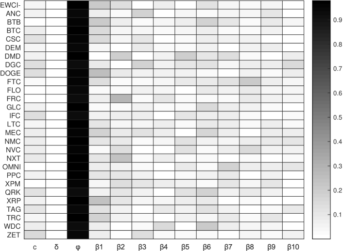
The third column in the Heatmap in Fig. 1 illustrates the value of . We find the parameter to be greater than 0.9 for all CCs and, for the most part, clearly close to 1. The latter is an important condition to be fulfilled for the assumption of a random walk ().
The augmented Dickey-Fuller test was performed for lags up to order ten. More complicated dynamics with serial correlation make themselves noticeable in the analysis by the fact that the coefficients of the terms corresponding to the lags are clearly different from zero. We find the absolute values of the coefficients (that means ) to be close to zero. In fact, the majority of the absolute coefficients are clearly smaller than 0.2 as an upper limit444By similar argumentation as in Wooldridge (2020, Chapter 11 therein) a repeated substitution causes the effectiveness of the corresponding terms to fall below the 5% mark in the next time step and thus become largely insignificant. and a basic model can be assumed (in Tab. 3 third column denoted with "G"). Only a few single coefficients exceed the value 0.2 by a small margin and in these cases a model with a slightly influencing lag structure with an average coefficient could be guessed at. By marking the corresponding CCs with "L", Tab. 3 shows for which CCs this is the case.
Due to the observed insignificance of the lag stucture, we assume a basic model "G" in these cases as well and expect statistical inaccuracies to distort the result due to the limited length of the time series. We therefore postulate a possible serial correlation in the data sets to be of minor importance. Thus, the detailed analysis of the results of the augmented Dickey-Fuller test suggests that the model cannot not be rejected for the returns . Here, denotes the individual time-constant drift term for each CC and, as above, denotes the innovation process.
Test on autoregressive conditional heteroscedasticity
The ARCH-Test is performed for time shifts up to the order of ten. Up to this lag, the null hypothesis that the innovation process of returns is homoscedastic could not be rejected for most CCs (see Tab. 3), i.e. the basic model with constant volatility and being an independent and identical distributed process with mean 0 and variance 1 could not be rejected for the majority of CCs. Note, that the results found in literature show a heterogeneous picture and we do not find ARCG effects in contrast to other related studies (Peng et al., 2018; Dyhrberg, 2016; Avital et al., 2014). After all, only 13 of 28 time series examined show ARCH effects and only in 8 cases clearly. The differences in studies may derive from different sampling frequencies or the differently chosen time period or its length and show that the design of the data collection may have an influence on the results.
| CC | ADF-Test | ARCH-Test | Distribution | |||
|---|---|---|---|---|---|---|
| ID | H0 | Model | -Value | H0 | -Value | |
| EWCI- | 0 | L | 29.4 | 1 | 0.0 | - |
| ANC | 0 | G | 11.7 | 0 | 6.6 | IID |
| BTB | 0 | L | 22.9 | 1 | 0.0 | - |
| BTC | 0 | G | 48.7 | 1 | 3.1 | IID |
| CSC | 0 | G | 49.2 | 0 | 50.8 | IID |
| DEM | 0 | G | 24.0 | 1 | 0.0 | - |
| DMD | 0 | G | 75.8 | 0 | 18.0 | IID |
| DGC | 0 | G | 11.0 | 1 | 0.0 | - |
| DOGE | 0 | L | 14.7 | 0 | 69.8 | IID |
| FTC | 0 | L | 14.9 | 1 | 0.0 | - |
| FLO | 1 | L | 4.0 | 0 | 63.2 | IID |
| FRC | 0 | L | 14.3 | 0 | 71.6 | IID |
| GLC | 0 | G | 65.2 | 0 | 16.6 | IID |
| IFC | 0 | G | 6.4 | 0 | 38.3 | IID |
| LTC | 0 | G | 34.2 | 0 | 25.2 | IID |
| MEC | 0 | G | 17.7 | 1 | 1.5 | IID |
| NMC | 0 | G | 42.0 | 0 | 38.1 | IID |
| NVC | 0 | G | 22.8 | 0 | 92.6 | IID |
| NXT | 0 | L | 50.4 | 1 | 0.0 | - |
| OMNI | 0 | G | 35.7 | 0 | 70.2 | IID |
| PPC | 0 | G | 41.5 | 1 | 0.4 | IID |
| XPM | 0 | G | 12.7 | 0 | 11.1 | IID |
| QRK | 1 | L | 2.0 | 1 | 0.3 | IID |
| XRP | 0 | L | 35.1 | 1 | 0.0 | - |
| TAG | 0 | G | 6.0 | 0 | 60.4 | IID |
| TRC | 0 | G | 46.0 | 1 | 1.9 | IID |
| WDC | 1 | L | 2.5 | 1 | 0.0 | - |
| ZET | 0 | G | 22.6 | 0 | 6.0 | IID |
The aforementioned results would justify the following calculation: and for the corresponding CCs. Estimates for the mean and the variance of the individual returns are noted in Tab. 2. Their calculation is also justified with the combined consideration of the test results described above.
Combining both tests, we have noted a characterization of the return distribution in the last column of Tab. 3. For the majority of CCs, independent and identical distributed (IID) returns can be assumed. Another part is approximately independent and identical distributed ( IID), because either the lag structure is less important in the ADF model or the rejection of homoscedasticity based on the -value is only weakly justified. For eight CCs the assumption of IID returns is clearly rejected.
Note, that the test for independently identical ditstributed returns could have been carried out with a turning point test (Bienaymé, 1874; Kendall and Stuart, 1977). However, as we are interested in a deeper analysis of the possible serial correlation in our data sets, we use a combination of the augmented Dickey-Fuller test and the ARCH-Test instead.
All tests carried out so far, do not reject the assumption that the returns obey an essentially symmetrical, unimodal distribution. Furthermore, for the majority of CCs the assumption of IID or nearly IID holds. In the first case (IID), the modeling of the empirical distribution with a distribution function is justified. In the second case ( IID), the model represents a coarser approximation. In the latter case, if the assumption of IID was to be rejected, the distribution function can only be used as a rough approximation and must be – just like the case ( IID) – examined more precisely and critically in individual cases as we show in the following section.
3.3 Determination of the appropriate return distribution function
When modeling the empirical distribution of returns, we focus on families of unimodal distribution functions that are defined over the entire axis (infinite support). Hence, a more detailed investigation of the following distribution functions suggests itself: normal distribution (N), the generalized extremvalue distribution (GED), the generalized logistic distribution type 0 and type 3 (GLD0, GLD3) and the SDI. The analysis below proves that the family of SDIs is the most promising for modeling the distribution of CC returns. Therefore, this family of functions will be introduced here in more detail. Several different parametrizations exist for the SDI. In the following formulation we follow the presentation and the SDI’s parametrization described in Nolan (2020, Def. 1.4 therein).
SDIs represent a class of distributions suitable for modeling heavy tails and skewness. A linear combination of two independent, identically and stable distributed random variables has the same distribution as the individual variables. A random variable follows the SDI if its characteristic function is given by:
| (2) |
The first parameter is called shape parameter and describes the tail of the distribution. This parameter may also be denoted as an index of stability or as a characteristic exponent. The second parameter is a skewness parameter. If , then the distribution is symmetric otherwise it is left-skewed () or right-skewed (). When is small, the skewness of is significant. As increases, the effect of decreases. Further, is called the scale parameter and is the location parameter.
For the special case the characteristic function Eq. (3.3) reduces to and becomes independent of the skewness parameter and the SDI becomes equal to N with mean and standard deviation .
Evaluation of distance measurements to compare model quality
In the following we use standard distance measures to determine and compare the model qualities of N, GED, GLD0, GLD3 and SDI for the individual CCs. There are several distance measures available which are suitable to measure the "discrepancy" between the empirical distribution function and a modelled distribution function. The distance measures from Cramér (1928) von Mises (1931) (-Distance), Anderson and Darling (1952, 1954) (-Distance) and Kolmogorov (1933) Smirnov (1936, 1948) (KS-Distance) are widely used in literature. A brief summary of the used distance measures are given in A.
In Tab. 4 we summarize the results for the Anderson Darling distance (). The results for the Kolmogorov Smirnov distance (KS) and the Cramér von Mises distance () are compiled in Tab. 11 and Tab. 10 in A.
| CC | Anderson Darling Distance | Best Choice | ||||
|---|---|---|---|---|---|---|
| ID | N | GED | GLD0 | GLD3 | SDI | |
| EWCI- | 3.41 | 147.4 | 1.76 | 0.81 | 0.79 | SDI |
| ANC | 8.65 | 22.4 | 2.53 | 1.61 | 0.39 | SDI |
| BTB | 3.36 | 12.3 | 0.76 | 0.48 | 0.22 | SDI |
| BTC | 2.07 | 224.8 | 0.88 | 0.60 | 0.97 | GLD3 |
| CSC | 21.80 | 42.6 | 3.90 | n.d. | 0.43 | SDI |
| DEM | 2.64 | 6.7 | 0.54 | 0.17 | 0.20 | GLD3 |
| DMD | 3.80 | 23.7 | 1.25 | 0.29 | 0.54 | GLD3 |
| DGC | 6.84 | 26.6 | 2.05 | 0.65 | 0.78 | GLD3 |
| DOGE | 9.56 | 9.1 | 4.10 | 1.77 | 0.53 | SDI |
| FTC | 9.41 | 14.2 | 1.77 | 1.05 | 0.17 | SDI |
| FLO | 1.74 | 1.5 | 0.54 | 0.54 | 0.32 | SDI |
| FRC | 17.36 | n.d. | 5.21 | 1.98 | 0.39 | SDI |
| GLC | 1.53 | 16.8 | 0.40 | 0.19 | 0.42 | GLD3 |
| IFC | n.d. | n.d. | 4.79 | 3.43 | 2.57 | SDI |
| LTC | 7.10 | 13.7 | 2.72 | 0.72 | 0.71 | SDI |
| MEC | 9.19 | 18.8 | 3.71 | 1.25 | 0.45 | SDI |
| NMC | 6.02 | 60.5 | 1.73 | 0.48 | 0.47 | SDI |
| NVC | 17.24 | 51.3 | 4.08 | 1.47 | 0.47 | SDI |
| NXT | 6.69 | 17.6 | 2.39 | 0.96 | 0.41 | SDI |
| OMNI | 1.25 | 4.4 | 0.25 | 0.24 | 0.24 | SDI |
| PPC | 4.93 | 31.9 | 1.63 | 0.61 | 0.48 | SDI |
| XPM | 5.66 | 5.0 | 1.53 | 0.67 | 0.27 | SDI |
| QRK | 6.32 | 9.5 | 2.12 | 0.53 | 0.52 | SDI |
| XRP | 13.90 | 13.0 | 5.71 | 2.79 | 0.62 | SDI |
| TAG | 4.85 | 5.4 | 1.23 | 0.30 | 0.64 | GLD3 |
| TRC | 4.36 | 5.5 | 0.80 | 0.45 | 0.13 | SDI |
| WDC | 9.68 | 24.1 | 3.95 | 1.35 | 0.57 | SDI |
| ZET | 5.23 | 12.3 | 1.58 | 0.41 | 0.48 | GLD3 |
The values of the various distance measures show that the GED is least suitable to model the empirical distribution function. This may derive from the fact that the GED contains a fundamental skewness, which can only be influenced slightly via a parameter selection. Further, as soon as the shape parameter becomes different from zero a fundamental change of the distribution model occurs and the definition interval on the -axis becomes restricted. Additionally, associated with a change of sign of the shape parameter there is a fundamental change of the distribution model as well and an abrupt change of the sign of the upper (or lower) bound on the -axis, see e.g. Embrechts et al. (1997). In the present case, these properties of the GED make it difficult to precisely adapt the distribution to the data set.
On closer inspection of the calculated distances, the N does not appear to be suitable as a model either, since it is neither suitable for the modeling of empirical distribution functions with fat tails nor for those with a slight skew. Overall, the GLD0 shows significantly smaller distances across all CCs, but is also not ideally suited, as it is completely symmetrical and is therefore not able to model any slight skewness. The best results in terms of the smallest distance can be achieved with the GLD3 and with the SDI. When comparing all CCs, the corresponding distances are very close to each other. If only the Cramér von Mises distance and the Kolmogorov Smirnov distance are considered, see A, it turns out that around half of the empirical distributions of CC returns can be modeled with one or the other distribution. But as soon as more attention is paid to the tail, i.e. if deviations in the tail area are to be weighted more heavily in order to account for tail risks, and the Anderson Darling distance is considered, the share of CCs, for which the SDI is the most suitable model, predominates.
This result ties in with the results of Majoros and Zempléni (2018); Kakinaka and Umeno (2020). Using intraday and daily time series for a small sample of CCs they show the SDI family to be the best choice for modeling the empirical distribution function of intraday and daily returns of CCs.
For a broader sample of CCs we found that the SDI is, on average, much better suited to model both slight skewness and pronounced tails in the empirical distribution function. Therefore we use the SDI for all CCs to model the distribution function of returns.
The stable distribution family as a model for cryptocurrencies
Tab. 5 shows the results of the parameter estimation for the SDI .
| CC | Parameter of the SDI | AD-Test | ||||||||
| ID | H0 | -Value | ||||||||
| EWCI- | 1.62 | 0.18 | 0.46 | 0.39 | 0.07 | 0.01 | -0.01 | 0.02 | 0 | 48.9 |
| ANC | 1.41 | 0.17 | 0.26 | 0.31 | 0.16 | 0.02 | -0.03 | 0.03 | 0 | 85.8 |
| BTB | 1.67 | 0.18 | 0.38 | 0.45 | 0.18 | 0.02 | -0.03 | 0.04 | 0 | 98.3 |
| BTC | 1.78 | 0.16 | -0.21 | 0.61 | 0.06 | 0.01 | 0.01 | 0.01 | 0 | 37.5 |
| CSC | 1.45 | 0.18 | 0.27 | 0.32 | 0.16 | 0.02 | -0.04 | 0.03 | 0 | 81.4 |
| DEM | 1.65 | 0.18 | -0.04 | 0.45 | 0.17 | 0.02 | -0.01 | 0.03 | 0 | 99.0 |
| DMD | 1.56 | 0.18 | 0.10 | 0.39 | 0.11 | 0.01 | -0.01 | 0.02 | 0 | 70.7 |
| DGC | 1.57 | 0.18 | 0.31 | 0.38 | 0.14 | 0.02 | -0.04 | 0.03 | 0 | 49.7 |
| DOGE | 1.33 | 0.17 | 0.35 | 0.27 | 0.08 | 0.01 | -0.02 | 0.02 | 0 | 72.0 |
| FTC | 1.63 | 0.18 | 0.54 | 0.38 | 0.12 | 0.01 | -0.05 | 0.03 | 0 | 99.7 |
| FLO | 1.88 | n.d. | 1.00 | n.d. | 0.16 | n.d. | -0.02 | n.d. | 0 | 92.3 |
| FRC | 1.24 | 0.16 | 0.06 | 0.26 | 0.13 | 0.02 | -0.02 | 0.03 | 0 | 86.0 |
| GLC | 1.80 | 0.16 | 0.43 | 0.63 | 0.15 | 0.02 | -0.02 | 0.03 | 0 | 82.5 |
| IFC | 1.47 | 0.18 | 0.25 | 0.33 | 0.12 | 0.01 | -0.04 | 0.02 | 1 | 4.6 |
| LTC | 1.37 | 0.17 | 0.06 | 0.30 | 0.06 | 0.01 | -0.01 | 0.01 | 0 | 55.2 |
| MEC | 1.25 | 0.16 | -0.01 | 0.26 | 0.09 | 0.01 | -0.02 | 0.02 | 0 | 79.9 |
| NMC | 1.48 | 0.18 | 0.07 | 0.34 | 0.08 | 0.01 | -0.01 | 0.02 | 0 | 78.0 |
| NVC | 1.42 | 0.17 | 0.28 | 0.31 | 0.08 | 0.01 | -0.03 | 0.02 | 0 | 77.5 |
| NXT | 1.48 | 0.18 | 0.37 | 0.32 | 0.10 | 0.01 | -0.03 | 0.02 | 0 | 83.8 |
| OMNI | 1.82 | 0.16 | 0.26 | 0.71 | 0.14 | 0.01 | -0.03 | 0.03 | 0 | 97.7 |
| PPC | 1.50 | 0.18 | 0.10 | 0.35 | 0.08 | 0.01 | -0.02 | 0.02 | 0 | 76.8 |
| XPM | 1.58 | 0.18 | 0.42 | 0.37 | 0.10 | 0.01 | -0.04 | 0.02 | 0 | 95.6 |
| QRK | 1.45 | 0.18 | 0.17 | 0.33 | 0.12 | 0.02 | -0.03 | 0.02 | 0 | 72.6 |
| XRP | 1.33 | 0.17 | 0.35 | 0.27 | 0.07 | 0.01 | -0.03 | 0.01 | 0 | 63.2 |
| TAG | 1.63 | 0.18 | 0.10 | 0.44 | 0.12 | 0.01 | -0.02 | 0.02 | 0 | 61.1 |
| TRC | 1.64 | 0.18 | 0.29 | 0.43 | 0.13 | 0.02 | -0.04 | 0.03 | 0 | 99.9 |
| WDC | 1.26 | 0.16 | 0.08 | 0.26 | 0.10 | 0.01 | -0.03 | 0.02 | 0 | 67.2 |
| ZET | 1.53 | 0.18 | 0.15 | 0.36 | 0.13 | 0.02 | -0.02 | 0.03 | 0 | 76.5 |
For the individual parameters of the SDI, the 95% scatter intervals are provided, as well. The latter can be determined from the covariance matrix of the estimated parameters. The covariance matrix of the parameter estimates is a matrix in which the off-diagonal element resembles the covariance between the estimates of the -th parameter and the -th parameter. For the CC FLO, these scatter intervals cannot be determined numerically using the data set at hand. This is due to the fact that the corresponding empirical distribution on the far right shows a very long, pronounced tail and is strongly skewed to the right. The estimated parameter of the SDI takes the value of 1 accordingly, see Tab. 5. It may be the case that the single right tail data point, i.e. the return in period 62, represents an outlier, which is difficult to determine and correct afterwards without any further knowledge.
On average, the estimated parameter exceeds 1.5. With parameter increasing to its limit value of 2.0, it can be seen that the distribution function becomes similar to the N and the skewness parameter () becomes increasingly insignificant. The parameters and of the SDI are mutually dependent and, as described above, the meaning of decreases when increases. So it is generally difficult to infer the skewness from the value alone. A relative comparison of the distributions with regard to the skewness is only possible if has the same value. Hence, for a more precise analysis of a distribution’s skewness, other methods are necessary. In this manner, we used the SIG-Test as an example and note the results in Tab. 2.
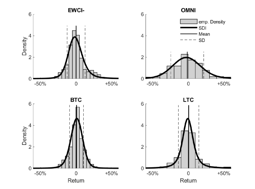
For some CCs and the EWCI- index, Fig. 2 shows the empirical densities and the density of the corresponding SDI in comparison.
In addition, the complete goodness of fit test according to Anderson Darling was carried out. The last two columns of Tab. 5 show that for almost all CCs with very high significance (high -values), the null hypothesis that the adjusted SDI models the data set cannot be rejected. Only for the CC Infinitecoin (IFC) this assumption is rejected at the 5% level. This is probably due to the fact that the empirical distribution suggests a slight bimodal distribution. This peculiarity of the CC Infinitecoin is also indicated in the results of the HDS-Test in Tab. 2.
Overall, it can be stated that the SDI family represents a suitable framework for modeling the distribution function of CC returns. We will make use of this finding for the assessment of tail risks and the comparison of our results with other modeling approaches.
4 Assessment of tail risks
4.1 Modeling of cryptocurrencies’ tail risks
Especially when considering high quantiles in the risk assessment process, separate modeling of the tail of the often unknown parent distribution is necessary. In practice, the GPD is used predominantly as a tail model (Basel Commitee on Banking Supervision, 2009). Henceforth, we briefly discuss the main steps of the tail modelling using the GPD in this section.
A theorem in extreme value theory, which goes back to Gnedenko (1943), Balkema and de Haan (1974) and Pickands III (1975), states that for a broad class of distributions, the distribution of the excesses over a threshold converges to a GPD if the threshold is sufficiently large.
The GPD is usually expressed as a two-parameter distribution and follows the distribution function:
| (3) |
where is a positive scale parameter and is a shape parameter (sometimes called the tail parameter). The density function is described as
| (4) |
with support for and when . The mean and variance are depicted as and , respectively. Thus, the mean and variance of the GPD are positive and finite only for and , respectively. For special values of , the GPD leads to various other distributions. When , the GPD translates to an exponential or a uniform distribution. For , the GPD has a long tail to the right and resembles a reparameterized version of the usual Pareto distribution. Several areas of applied statistics have used the latter range of to model data sets that exhibit this form of a long tail.
Since the GPD was introduced by Pickands III (1975), numerous theoretical advancements and applications have followed (Davison (1984), Smith (1984), Smith (1985), van Montfort and Witter (1985), Hosking and Wallis (1987), Davison and Smith (1990), Choulakian and Stephens (2001)). Its applications include the use in analysis of extreme events in hydrology, as a failure-time distribution in reliability studies and in the modeling of large insurance claims. Numerous examples of applications can be found in Embrechts et al. (1997) and the studies listed therein. The GPD is also increasingly used in financial and banking sectors. Especially in the assessment of risks based on high quantiles, the GPD is one of the proposed distributions for modeling the tail of an unknown parent distribution (Basel Commitee on Banking Supervision, 2009).
The preferred method in literature for estimating the parameters of the GPD is the standard maximum likelihood method (Davison (1984), Smith (1984), Smith (1985), Hosking and Wallis (1987)). Choulakian and Stephens (2001) state that it is theoretically possible to have data sets for which no solution to the likelihood equations exists, however this appears to be an extremly rare case in practice. In fact, in our examination of the 27 CCs and the EWCI-, maximum likelihood estimates of the parameters could be deduced in every case. Nevertheless, a plausibility check of the results is highly recommended. As we show in Sec. 4.2, when assessing tail risks, it is advisable to evaluate the results, in order to avoid possible misinterpretations in single individual cases.
For the separate modeling of the tail, solely the parameters of the GPD need to be determined from the data pertaining to the tail region of the underlying empirical distribution function, i.e. the data which belong to the area below a threshold in case of the loss tail.
Tab. 6 depicts the estimated parameters for the GPD for the different CCs. The second column gives the proportion of the whole dataset belonging to the loss tail. The proportion of the return data below the threshold is used to fit the parameters of the GPD. The threshold value lies within the bandwidth shown in Tab. 2 and when considering the loss tail closer to the lower interval limit of the bandwidth. Due to the standard goodness of fit tests according to Crámer von Mises (CvM) or Anderson Darling (AD), the null hypothesis that the GPD is a suitable model for the tail, can not be rejected on any significance level. In addition, the -values for the lower tail statistics (LT) according to Ahmad et al. (1988) are given in Tab. 6. The corresponding statistics is defined in B and used here to determine the threshold value . As can be seen in column six of Tab. 6 the lower tail statistics show high confidence levels, as well.
| CC | Prop. | GPD-Parameter | Goodness of Fit | ||||
|---|---|---|---|---|---|---|---|
| ID | -Values | ||||||
| LT | CvM | AD | |||||
| EWCI- | 45.7 | -1.7 | -0.09 | 0.09 | 88.0 | 84.9 | 92.6 |
| ANC | 4.3 | -52.0 | -0.08 | 0.61 | 98.5 | 98.1 | 93.9 |
| BTB | 4.3 | -51.0 | 0.63 | 0.13 | 99.0 | 96.1 | 98.1 |
| BTC | 24.1 | -3.9 | -0.30 | 0.10 | 93.0 | 97.5 | 98.1 |
| CSC | 9.9 | -35.5 | 0.82 | 0.11 | 96.7 | 99.7 | 94.3 |
| DEM | 51.4 | -1.3 | -0.05 | 0.22 | 54.2 | 58.2 | 60.8 |
| DMD | 4.3 | -32.5 | 0.04 | 0.13 | 94.5 | 89.0 | 93.2 |
| DGC | 10.3 | -31.7 | 0.61 | 0.08 | 99.8 | 99.6 | 99.5 |
| DOGE | 21.6 | -9.2 | 0.13 | 0.09 | 99.1 | 99.4 | 98.9 |
| FTC | 3.5 | -37.0 | 0.99 | 0.05 | 99.7 | 99.4 | 93.7 |
| FLO | 16.3 | -20.3 | -0.25 | 0.17 | 93.9 | 91.5 | 89.2 |
| FRC | 11.0 | -28.8 | 0.28 | 0.31 | 98.8 | 98.3 | 99.6 |
| GLC | 51.8 | 0.2 | -0.19 | 0.20 | 99.9 | 99.9 | 100.0 |
| IFC | 20.9 | -18.2 | 0.55 | 0.07 | 55.0 | 70.4 | 52.8 |
| LTC | 44.3 | -0.7 | -0.18 | 0.11 | 57.5 | 67.7 | 54.1 |
| MEC | 56.4 | 0.0 | 0.16 | 0.12 | 99.8 | 99.2 | 93.3 |
| NMC | 46.1 | -1.9 | 0.15 | 0.09 | 78.0 | 95.7 | 94.0 |
| NVC | 9.2 | -19.3 | 0.72 | 0.05 | 77.2 | 93.6 | 86.0 |
| NXT | 2.8 | -34.6 | 1.27 | 0.03 | 60.1 | 76.7 | 67.7 |
| OMNI | 15.2 | -23.0 | -0.11 | 0.14 | 95.9 | 96.2 | 97.1 |
| PPC | 8.5 | 21.3 | 0.00 | 0.09 | 96.7 | 97.1 | 98.8 |
| XPM | 4.6 | 29.5 | -0.08 | 0.12 | 91.4 | 93.1 | 96.7 |
| QRK | 63.5 | -1.6 | 0.05 | 0.16 | 47.7 | 60.8 | 61.1 |
| XRP | 2.8 | -25.6 | 0.76 | 0.04 | 99.2 | 98.8 | 99.1 |
| TAG | 53.2 | -0.5 | -0.13 | 0.17 | 91.2 | 92.7 | 96.8 |
| TRC | 35.5 | -9.9 | -0.06 | 0.15 | 64.2 | 70.9 | 81.0 |
| WDC | 62.8 | 0.8 | 0.18 | 0.13 | 94.8 | 94.4 | 88.9 |
| ZET | 20.9 | -17.8 | 0.27 | 0.11 | 59.8 | 83.6 | 82.5 |
4.2 Risk assessment at high quantiles
In this section, we use the SDI as the body model and the GPD as the tail model to determine the risk parameters Value at Risk (as a quantile) and the Conditional Value at Risk (as a weighted loss when the loss threshold is exceeded), see i.a. Embrechts et al. (1997); Hull (2018). The data set includes return observations for each CC, so that a comparison of the results with the empirically determined values is possible for moderately large confidence levels (). The corresponding values for the confidence level of 99.9%, which is important for regulatory purposes (Basel Commitee on Banking Supervision, 2004; European Parliament, 2009, 2013a, 2013b), can only be estimated for data records of this length using a previously fitted body or tail model. The calculation of the quantiles is also subject to a statistical spread and the estimation error increases the fatter the tail is and the higher the confidence level is selected, see e.g. Hoffmann and Börner (2020b).
Value at Risk
Tab. 7 illustrates the results of the risk assessment for the most common confidence levels found in literature and regulatory requirements. The Value at Risk for the observed CCs are shown for the various model.
| CC | Value at Risk | |||||||||||
|---|---|---|---|---|---|---|---|---|---|---|---|---|
| empirical | Tail-Modell (GPD) | Body-Modell (SDI) | ||||||||||
| ID | 95% | 97% | 99% | 99.9% | 95% | 97% | 99% | 99.9% | 95% | 97% | 99% | 99.9% |
| EWCI- | 26 | 29 | 38 | 41 | 19 | 23 | 30 | 43 | 18 | 22 | 33 | 116 |
| ANC | 101 | 133 | 212 | 241 | 42 | 73 | 136 | 252 | 46 | 60 | 119 | 582 |
| BTB | 75 | 91 | 154 | 201 | 49 | 56 | 82 | 251 | 47 | 55 | 82 | 276 |
| BTC | 21 | 24 | 28 | 30 | 16 | 19 | 24 | 31 | 15 | 18 | 28 | 91 |
| CSC | 117 | 166 | 424 | 698 | 46 | 58 | 110 | 595 | 47 | 61 | 116 | 535 |
| DEM | 72 | 84 | 100 | 101 | 51 | 61 | 82 | 122 | 48 | 60 | 100 | 367 |
| DMD | 44 | 52 | 72 | 85 | 30 | 37 | 52 | 85 | 30 | 38 | 69 | 280 |
| DGC | 65 | 82 | 153 | 217 | 39 | 46 | 71 | 229 | 40 | 49 | 81 | 314 |
| DOGE | 36 | 43 | 56 | 61 | 23 | 29 | 42 | 77 | 23 | 31 | 64 | 343 |
| FTC | 50 | 60 | 109 | 145 | 36 | 38 | 50 | 205 | 32 | 37 | 53 | 177 |
| FLO | 49 | 54 | 66 | 68 | 38 | 44 | 55 | 70 | 37 | 42 | 52 | 68 |
| FRC | 110 | 142 | 256 | 332 | 57 | 78 | 136 | 333 | 54 | 79 | 185 | 1159 |
| GLC | 49 | 55 | 68 | 74 | 38 | 44 | 56 | 74 | 36 | 42 | 56 | 140 |
| IFC | 61 | 77 | 114 | 126 | 34 | 43 | 75 | 251 | 35 | 45 | 82 | 365 |
| LTC | 27 | 31 | 34 | 34 | 20 | 24 | 31 | 41 | 21 | 30 | 62 | 321 |
| MEC | 59 | 71 | 99 | 113 | 37 | 46 | 70 | 137 | 38 | 56 | 128 | 787 |
| NMC | 42 | 50 | 92 | 110 | 27 | 34 | 51 | 97 | 25 | 33 | 63 | 284 |
| NVC | 47 | 63 | 141 | 236 | 23 | 28 | 46 | 188 | 24 | 31 | 59 | 278 |
| NXT | 42 | 48 | 78 | 84 | 33 | 34 | 42 | 210 | 27 | 33 | 59 | 258 |
| OMNI | 48 | 55 | 67 | 73 | 37 | 43 | 55 | 76 | 37 | 42 | 56 | 142 |
| PPC | 35 | 40 | 55 | 60 | 26 | 31 | 41 | 61 | 25 | 33 | 60 | 258 |
| XPM | 40 | 46 | 62 | 68 | 29 | 35 | 47 | 70 | 27 | 33 | 51 | 191 |
| QRK | 62 | 71 | 91 | 94 | 41 | 50 | 70 | 117 | 38 | 50 | 96 | 440 |
| XRP | 30 | 36 | 57 | 73 | 24 | 25 | 32 | 85 | 22 | 30 | 61 | 330 |
| TAG | 47 | 53 | 62 | 64 | 35 | 41 | 53 | 73 | 34 | 42 | 69 | 252 |
| TRC | 51 | 57 | 69 | 73 | 37 | 44 | 57 | 83 | 36 | 44 | 68 | 238 |
| WDC | 64 | 79 | 109 | 122 | 39 | 50 | 76 | 150 | 40 | 57 | 128 | 769 |
| ZET | 59 | 73 | 91 | 98 | 37 | 46 | 70 | 151 | 37 | 47 | 85 | 357 |
Overall, it can be seen that in the overwhelming number of individual cases, the assessment of risk with the tail model (GPD) is closer to the empirical Value at Risk values. This applies to the lower confidence levels in particular, but even with high confidence level of 99.9%, better estimates are possible in individual cases compared to the body model. This becomes apparent from the statistical parameters of the deviation analysis shown in Tab. 8 as well. The mean value and standard deviation over the set of CCs are shown. For this purpose, the deviation between the modeled variable and the corresponding empirical Value at Risks was determined. It turns out that, on average, adjusting the GPD as tail model leads to better risk estimates.
| VaR | Confidence levels | ||||||
|---|---|---|---|---|---|---|---|
| 95% | 97% | 99% | 99.9% | ||||
| Mean | GPD | ./. | Emp. | 0.5 | -0.2 | -4.6 | 15.5 |
| SDI | ./. | Emp. | -0.3 | 0.4 | 10.5 | 214.1 | |
| SD | GPD | ./. | Emp. | 2.4 | 2.1 | 7.3 | 43.1 |
| SDI | ./. | Emp. | 1.8 | 4.1 | 19.3 | 211.7 | |
When comparing CCs with each other, a heterogeneous picture emerges, see Tab. 7. If the empirical Value at Risk for the 99.9% confidence interval is taken as a measure, two subgroups can be defined for the cut-off value 100%. One group possesses a significantly lower tail risk ( 100%) as the corresponding values in Tab. 6 indicate. The other group ( 100 %) partly embodies a significantly higher tail risk. Correspondingly, large values can be determined for these CCs.
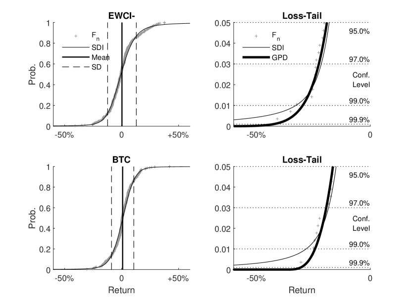
Fig. 3 shows the empirical distribution function for the EWCI- and Bitcoin (BTC), the SDI as a body model and the GPD as a tail model in comparison. The graphics on the right portray an enlargement of the loss area. Particularly in this region, the GPD models the empirical distribution function very well. Considering the afore conducted analysis, it can be stated that the GPD is ideally suited to carry out risk assessment at high quantiles. Therefore, we exclusively consider the GPD to estimate the Conditional Value at Risk as a further risk indicator in the following.
Conditional Value at Risk
The following Tab. 9 shows the Conditional Value at Risk calculated with the tail model (see Tab. 6) for the individual CCs. The calculation of the Conditional Value at Risk can be conducted using the mean excess function of the GPD:
| (5) |
with greater than the lower bound of the definition interval of the GPD considering the loss tail and the parameters of the GPD. The mean excess function is bound to the restrictions: , and , see e.g. Embrechts et al. (1997, Theorem 3.4.13). In Tab. 9 we used Eq. (5) to estimate the Conditional Value at Risk for each CCs setting .
Once more, the grouping of CCs described above can be seen. A group of CCs with a fat tail and therefore higher tail risk can be distinguished from a group with moderate risk, see Tab. 9.
| CC | Conditional Value at Risk | |||
|---|---|---|---|---|
| ID | 95% | 97% | 99% | 99.9% |
| EWCI- | 25 | 29 | 35 | 47 |
| ANC | 96 | 125 | 184 | 292 |
| BTB | 169 | 188 | 258 | 717 |
| BTC | 20 | 23 | 26 | 31 |
| CSC | 308 | 374 | 655 | 3294 |
| DEM | 70 | 79 | 99 | 138 |
| DMD | 45 | 52 | 68 | 102 |
| DGC | 118 | 136 | 200 | 600 |
| DOGE | 37 | 43 | 59 | 98 |
| FTC | 3219 | 3408 | 4343 | 16648 |
| FLO | 44 | 49 | 58 | 69 |
| FRC | 122 | 151 | 231 | 504 |
| GLC | 49 | 54 | 64 | 79 |
| IFC | 91 | 112 | 181 | 571 |
| LTC | 26 | 29 | 35 | 44 |
| MEC | 59 | 70 | 99 | 178 |
| NMC | 43 | 51 | 71 | 125 |
| NVC | 99 | 115 | 180 | 679 |
| NXT | -134 | -138 | -165 | -784 |
| OMNI | 46 | 51 | 62 | 80 |
| PPC | 35 | 40 | 49 | 70 |
| XPM | 38 | 43 | 55 | 76 |
| QRK | 59 | 69 | 90 | 140 |
| XRP | 114 | 121 | 147 | 367 |
| TAG | 46 | 52 | 62 | 80 |
| TRC | 49 | 55 | 68 | 92 |
| WDC | 63 | 76 | 107 | 197 |
| ZET | 66 | 79 | 112 | 223 |
Furthermore, two peculiarities are noticeable concerning the CCs Feathercoin (FTC) and Nxt (NXT). For both CCs, the tail is modeled on a small number of data points which have been assigned to the tail. This individual property of the data set deriving from the random distribution of the data in the tail area, is assumed to be given and, as already noted, is not corrected. In particular, when estimating the parameter , small samples lead to large statistical errors. Regrading the conspicuous CCs, it can be observed that the parameter is very close to 1 in one case (FTC) and even higher in the other case (NXT), see Tab. 6. As a result, the calculation of the Conditional Value at Risk for the CC NXT is not possible and must be discarded, cf. Eq. (5) and the restriction . On the other hand, the calculation of the FTC with has to be questioned critically. Hence, the Conditional Value at Risk may only be a rough estimate in this case.
5 Conclusion
This study aims to find a distribution which models CC returns most accurateley and does not suffer from restrictions in specific parts of the distribution. In former research the SDI and GPD have been found to model the body or the tail of the CC return distributions adequately respectively. Nevertheless both distributions prove to be unsuitable to model the entirety of the distrubition appropriately. Therefore, using a novel approach to separate of distribution’s tail from its body, we model the entire distribution by combining the model abilities of the SDI for the body and the GPD for the tail.
We select 27 CCs from the broad market of CCs according to predefined criteria and construct the representative index EWCI-. Overall, we find independent, identical distribution like the GPD and the SDI to be well suited for the most part and the family of SDIs in particular to be able to model the slightly skewed empirical distributions especially in the body region. A comparison between different distribution functions shows that the SDI has outstanding modeling properties across the entire data set. However, we show that the assessment of risks associated with fat tails can be carried out more precisely with the GPD. The analysis of tail risks in the CC market using the GPD further hints towards a certain internal structure of the CC market. It turns out that the CC market can roughly be divided into two sets: CCs with moderate risk and CCs with high risk. This finding provides valuable information for both investors and regulators alike. Hence, our results are not only relevant for scientific applications and extensions but for conceivable future regulation as well, if the asset class of CC is to become a permanent, noteworthy component of institutional investors’ portfolios in the financial sector in the future. In this regard, numerous future extensions and topics of research are conveivable. On the one hand, the SDI’s suitability to model CC returns in portfolio optimization remains to be investigated. On the other hand, further research considering the segmentation of the CC market could enrich the understanding of CCs and improve forecasts concerned with the fundamental behavior of different CCs.
Appendix A Distance measures – Tables of results
A.1 Distance measures
In what follows a brief summary of the used distance measures is given.
Cramér von Mises and Anderson Darling distance measures
As a convenient measure of the distance or "discrepancy" between the empirical distribution functions due to Kolmogorov (1933) and a model , usually the weighted mean square error is considered
| (6) |
which was introduced in the context of statistical test procedures by Cramér (1928), von Mises (1931) and Smirnov (1936); compare also Shorack and Wellner (2009) and the references therein. In decision theory (Ferguson, 1967), the weighted mean square error has broad applicability in the determination of the unknown parameters of distributions via minimum distance methods (Wolfowitz, 1957; Blyth, 1970; Parr and Schucany, 1980; Boos, 1982). This measure of error is also used when adapting tail models (Hoffmann and Börner, 2020a, 2021). Therefore, in Sec. 4.1 we applied this error measure in connection with the adaption of a suitable tail model for CC returns. A brief overview of the procedure to fit a suitable tail model is given in B.
The non-negative weight function in Eq. (6) is a suitable preassigned function for accentuating the difference between the distribution functions in the range where the distance measure is desired to have sensitivity. Consider the weight function
| (7) |
for real-valued stress parameters and . Here, affects the weight at the lower tail and at the upper tail. Then, for , Eq. (6) provides the Cramér von Mises distance used in the corresponding statistic (Cramér, 1928; von Mises, 1931), whereas when heavily weighting the tails (), it is equal to the Anderson Darling distance used in the corresponding statistic (Anderson and Darling, 1952, 1954). The Anderson Darling distance weights the difference between the two distributions simultaneously more heavily at both ends of the distribution .
Cramér von Mises Distance
| CC | Cramér von Mises Distance | Best Choice | ||||
|---|---|---|---|---|---|---|
| ID | N | GED | GLD0 | GLD3 | SDI | |
| EWCI- | 0.62 | 29.89 | 0.23 | 0.07 | 0.12 | GLD3 |
| ANC | 1.51 | 4.25 | 0.41 | 0.24 | 0.06 | SDI |
| BTB | 0.55 | 2.22 | 0.11 | 0.06 | 0.04 | SDI |
| BTC | 0.40 | 41.81 | 0.16 | 0.11 | 0.19 | GLD3 |
| CSC | 3.94 | 8.22 | 0.60 | 0.15 | 0.09 | SDI |
| DEM | 0.43 | 1.20 | 0.08 | 0.02 | 0.04 | GLD3 |
| DMD | 0.70 | 5.19 | 0.22 | 0.05 | 0.10 | GLD3 |
| DGC | 1.21 | 5.33 | 0.33 | 0.06 | 0.14 | GLD3 |
| DOGE | 1.86 | 1.70 | 0.64 | 0.20 | 0.07 | SDI |
| FTC | 1.54 | 2.37 | 0.21 | 0.09 | 0.03 | SDI |
| FLO | 0.29 | 0.23 | 0.07 | 0.07 | 0.05 | SDI |
| FRC | 3.26 | 6.35 | 0.94 | 0.33 | 0.07 | SDI |
| GLC | 0.27 | 3.66 | 0.06 | 0.02 | 0.08 | GLD3 |
| IFC | 2.92 | 4.43 | 0.91 | 0.72 | 0.58 | SDI |
| LTC | 1.35 | 2.98 | 0.46 | 0.11 | 0.12 | GLD3 |
| MEC | 1.75 | 3.78 | 0.67 | 0.22 | 0.06 | SDI |
| NMC | 1.11 | 13.40 | 0.32 | 0.08 | 0.09 | GLD3 |
| NVC | 3.09 | 10.46 | 0.65 | 0.17 | 0.09 | SDI |
| NXT | 1.20 | 3.57 | 0.33 | 0.09 | 0.07 | SDI |
| OMNI | 0.18 | 0.84 | 0.03 | 0.04 | 0.04 | GLD0 |
| PPC | 0.88 | 7.07 | 0.26 | 0.09 | 0.08 | SDI |
| XPM | 0.99 | 0.86 | 0.20 | 0.05 | 0.05 | SDI |
| QRK | 1.15 | 1.74 | 0.36 | 0.08 | 0.10 | GLD3 |
| XRP | 2.57 | 2.44 | 0.79 | 0.28 | 0.09 | SDI |
| TAG | 0.87 | 0.94 | 0.22 | 0.04 | 0.13 | GLD3 |
| TRC | 0.71 | 0.96 | 0.09 | 0.04 | 0.02 | SDI |
| WDC | 1.80 | 5.03 | 0.70 | 0.23 | 0.10 | SDI |
| ZET | 0.92 | 2.33 | 0.25 | 0.05 | 0.09 | GLD3 |
Kolmogorov Smirnov distance measure
Furthermore, we also determine the well-known distance between the empirical distribution function and the distribution model due to Kolmogorov (1933) and Smirnov (1936, 1948). The Kolmogorov Smirnov distance (KS) calculates the supremum of the absolute difference between the empirical and the estimated distribution functions. Hence, the Kolmogorov Smirnov distance quantifies the "discrepancy" between the empirical distribution function of returns and the cumulative distribution function of the reference distribution, i.e. the model of the distribution function of CC returns s. A more theoretical overview and comparisons to other distance measures can be found in, e.g. Stephens (1974); Shorack and Wellner (2009).
Kolmogorov Smirnov Distance
| CC | Kolmogorov Smirnov Distances KS | Best Choice | ||||
|---|---|---|---|---|---|---|
| ID | N | GED | GLD0 | GLD3 | SDI | |
| EWCI- | 0.100 | 0.509 | 0.063 | 0.043 | 0.051 | GLD3 |
| ANC | 0.132 | 0.233 | 0.069 | 0.070 | 0.047 | SDI |
| BTB | 0.087 | 0.156 | 0.056 | 0.037 | 0.042 | GLD3 |
| BTC | 0.077 | 0.591 | 0.058 | 0.047 | 0.060 | GLD3 |
| CSC | 0.179 | 0.296 | 0.085 | 0.053 | 0.047 | SDI |
| DEM | 0.071 | 0.127 | 0.048 | 0.027 | 0.039 | GLD3 |
| DMD | 0.094 | 0.233 | 0.056 | 0.039 | 0.050 | GLD3 |
| DGC | 0.117 | 0.241 | 0.066 | 0.034 | 0.045 | GLD3 |
| DOGE | 0.159 | 0.132 | 0.099 | 0.053 | 0.042 | SDI |
| FTC | 0.134 | 0.141 | 0.061 | 0.045 | 0.031 | SDI |
| FLO | 0.069 | 0.060 | 0.036 | 0.035 | 0.038 | GLD3 |
| FRC | 0.166 | 0.250 | 0.097 | 0.061 | 0.047 | SDI |
| GLC | 0.072 | 0.190 | 0.038 | 0.025 | 0.040 | GLD3 |
| IFC | 0.194 | 0.251 | 0.142 | 0.144 | 0.106 | SDI |
| LTC | 0.133 | 0.184 | 0.077 | 0.043 | 0.058 | GLD3 |
| MEC | 0.144 | 0.206 | 0.096 | 0.070 | 0.041 | SDI |
| NMC | 0.095 | 0.368 | 0.056 | 0.040 | 0.037 | SDI |
| NVC | 0.167 | 0.338 | 0.092 | 0.052 | 0.042 | SDI |
| NXT | 0.134 | 0.196 | 0.077 | 0.051 | 0.039 | SDI |
| OMNI | 0.052 | 0.113 | 0.028 | 0.031 | 0.036 | GLD0 |
| PPC | 0.109 | 0.262 | 0.063 | 0.048 | 0.053 | GLD3 |
| XPM | 0.116 | 0.095 | 0.055 | 0.048 | 0.035 | SDI |
| QRK | 0.108 | 0.139 | 0.073 | 0.048 | 0.048 | SDI |
| XRP | 0.171 | 0.168 | 0.101 | 0.061 | 0.039 | SDI |
| TAG | 0.101 | 0.103 | 0.056 | 0.037 | 0.048 | GLD3 |
| TRC | 0.099 | 0.120 | 0.039 | 0.033 | 0.023 | SDI |
| WDC | 0.144 | 0.236 | 0.103 | 0.075 | 0.052 | SDI |
| ZET | 0.123 | 0.154 | 0.077 | 0.049 | 0.047 | SDI |
Appendix B Modelling the tail of a distribution
For a very large class of parent distribution functions, the GPD can be used as a model for the tail, cf., e.g., Embrechts et al. (1997). This class of distributions includes all common parent distributions that play a role in the financial sector. Because of that, almost no uncertainty exists regarding the model selection for the tail of the unknown parent distribution. The required quantiles can then be determined to high confidence levels with sufficient certainty. A certain threshold thus divides the parent distribution into two areas: a body and a tail region. This approach is already common practice for calculating high quantiles more accurately, as indicated in European Parliament (2009).
Various authors have proposed methods for determining the appropriate threshold and subsequently the GPD as model for the tail from empirical data. Most methods require the setting of parameters, which often requires experience and hinders full automation of the modeling process. Based on ideas from Huisman et al. (2001); Longin and Solnik (2001); Chapelle et al. (2005); Crama et al. (2007); Hoffmann and Börner (2018, 2020a) we use the following method for the determination of the tail model.
Given a suitable distance measure as a function of the estimated GPD as a tail model and the empirical distribution function due to Kolmogorov (1933), an automated modeling process can be constructed using the following algorithm.
-
1.
Sort the random sample taken from an unknown parent distribution in descending order: .
-
2.
Let , and find, for each , the estimates of the parameters of the GPD. Note: For numerical reasons, we start at k = 2.
-
3.
Calculate the probabilities for with the estimated GPD, and determine the distance for .
-
4.
Find the index of the minimum of the distance .
Then, the optimal threshold value is estimated by , and the model of the tail of the unknown parent distribution is given by the estimated GPD , which itself is determined from the subset .
Chapelle et al. (2005) suggest using the mean squared error (MSE) as distance measure . Bader et al. (2018) implement a different algorithm based on sequences of goodness-of-fit tests. They use the Cramér-von Mises statistic and the Anderson-Darling statistic in combination with some beforehand set stopping rules. In contrast, we use the statistics (lower tail) or its counterpart (upper tail) due to Ahmad et al. (1988) as distance measure in the algorithm above.
The aforementioned distance measures are basing on the the weighted mean square error Eq. (6) The distance measures due to Ahmad et al. (1988) are derived from Eq. (6) when the integral is calculated with the weight functions Eq. (7) and for the lower tail (= ) and for the upper tail (= ).
This choice is justified as follows: The distance measure should take more account of the deviations between the measured data and the modeled data, especially in the tail area. This can be achieved with the asymmetrical weight functions – mentioned above – used in the weighted mean square error as distance measure , cf. e.g. Hoffmann and Börner (2018, 2020a). So, the distance measures and of Ahmad et al. (1988) take into account precisely the required asymmetrical weighting.
The pseudocode shown above was recently implemented in software packages and is available free of charge as a Python or R package, cf. Zitate, Links. The analysis shown in the main part was carried out with this packages.
References
- Ahmad et al. (1988) Ahmad, M.I., Sinclair, C.D., Spurr, B.D., 1988. Assessment of flood frequency models using empirical distribution function statistics. Water Resources Research 24, 1323–1328. doi:10.1029/WR024i008p01323.
- Anderson and Darling (1952) Anderson, T.W., Darling, D.A., 1952. Asymptotic theory of certain "goodness of fit" criteria based on stochastic processes. The Annals of Mathematical Statistics 23, 193–212. doi:10.1214/aoms/1177729437.
- Anderson and Darling (1954) Anderson, T.W., Darling, D.A., 1954. A test of goodness of fit. Journal of the American Statistical Association 49, 765–769. doi:10.2307/2281537.
- Avital et al. (2014) Avital, M., Leimeister, J.M., Schultze, U., 2014. ECIS 2014 proceedings: 22th European Conference on Information Systems ; Tel Aviv, Israel, June 9-11, 2014. AIS Electronic Library. URL: http://aisel.aisnet.org/ecis2014/.
- Bader et al. (2018) Bader, B., Yan, J., Zhang, X., 2018. Automated threshold selection for extreme value analysis via goodness-of-fit tests with application to batched return level mapping. The Annals of Applied Statistics 12, 310–329.
- Balcilar et al. (2017) Balcilar, M., Bouri, E., Gupta, R., Roubaud, D., 2017. Can volume predict bitcoin returns and volatility? a quantiles-based approach. Economic Modelling 64, 74–81. doi:10.1016/J.ECONMOD.2017.03.019.
- Balkema and de Haan (1974) Balkema, A.A., de Haan, L., 1974. Residual life time at great age. The Annals of Probability 2, 792–804. doi:10.1214/aop/1176996548.
- Basel Commitee on Banking Supervision (2004) Basel Commitee on Banking Supervision, 2004. International convergence of capital measurement and capital standards - a revised framework.
- Basel Commitee on Banking Supervision (2009) Basel Commitee on Banking Supervision, 2009. Observed range of practice in key elements of advanced measurement approaches (ama).
- Baur et al. (2018) Baur, D.G., Dimpfl, T., Kuck, K., 2018. Bitcoin, gold and the us dollar–a replication and extension. Finance Research Letters 25, 103–110.
- Bienaymé (1874) Bienaymé, I.J., 1874. Sur une question de probabilités. Bulletin de la Société Mathématique de France 2, 153–154.
- Blyth (1970) Blyth, C.R., 1970. On the inference and decision models of statistics. The Annals of Mathematical Statistics 41, 1034–1058.
- Boos (1982) Boos, D.D., 1982. Minimum anderson-darling estimation. Communication in Statistics-Theory and Methods 11, 2747–2774.
- Bouri et al. (2017a) Bouri, E., Gupta, R., Tiwari, A.K., Roubaud, D., 2017a. Does bitcoin hedge global uncertainty? evidence from wavelet-based quantile-in-quantile regressions. Finance Research Letters 23, 87–95. doi:10.1016/j.frl.2017.02.009.
- Bouri et al. (2017b) Bouri, E., Molnár, P., Azzi, G., Roubaud, D., Hagfors, L.I., 2017b. On the hedge and safe haven properties of bitcoin: Is it really more than a diversifier? Finance Research Letters 20, 192–198. doi:10.1016/j.frl.2016.09.025.
- Brauneis and Mestel (2018) Brauneis, A., Mestel, R., 2018. Price discovery of cryptocurrencies: Bitcoin and beyond. Economics Letters 165, 58–61.
- Brière et al. (2015) Brière, M., Oosterlinck, K., Szafarz, A., 2015. Virtual currency, tangible return: Porfolio diversification with bitcoin. Journal of Asset Management 16, 365–373.
- Cantelli (1933) Cantelli, F.P., 1933. Sulla determinazione empirica delle leggi di probabilità. Giornale dell’Istituto Italiano degli Attuari 1933, 421–424.
- Caporale et al. (2018) Caporale, G.M., Gil-Alana, L., Plastun, A., 2018. Persistence in the cryptocurrency market. Research in International Business and Finance 46, 141–148. doi:10.1016/j.ribaf.2018.01.002.
- Chapelle et al. (2005) Chapelle, A., Crama, Y., Hübner, G., Peters, J., 2005. Measuring and managing operational risk in financial sector: An integrated framework. Social Science Research Network Electronic Journal doi:10.2139/ssrn.675186.
- Choulakian and Stephens (2001) Choulakian, V., Stephens, M.A., 2001. Goodness-of-fit tests for the generalized pareto distribution. Technometrics 43, 478–484.
- Corbet et al. (2019) Corbet, S., Lucey, B., Urquhart, A., Yarovaya, L., 2019. Cryptocurrencies as a financial asset: A systematic analysis. International Review of Financial Analysis 62, 182–199. doi:10.1016/j.irfa.2018.09.003.
- Corbet et al. (2018) Corbet, S., Lucey, B.M., Peat, M., Vigne, S., 2018. Bitcoin futures - what use are they? Economics Letters 172, 23–27.
- Crama et al. (2007) Crama, Y., Hübner, G., Peters, J. (Eds.), 2007. Impact of the collection threshold on the determination of the capital charge for operational risk: Advances in Risk Management. Palgrave Macmillan, New York.
- Cramér (1928) Cramér, H., 1928. On the composition of elementary errors: Second paper: Statistical applications. Scandinavian Actuarial Journal 1, 141–180.
- Davison (1984) Davison, A.C., 1984. Modelling excess over high threshold, with an application: Statistical Extremes and Applications. Reidel Publishing Company, Dordrecht, Netherlands. doi:10.1007/978-94-017-3069-3{\textunderscore}34.
- Davison and Smith (1990) Davison, A.C., Smith, R.L., 1990. Models for exceedances over high thresholds (with comments). Journal of the Royal Statistical Society, Series B (Methodological) 52, 393–442.
- Dickey and Fuller (1979) Dickey, D.A., Fuller, W.A., 1979. Distribution of the estimators for autoregressive time series with a unit root. Journal of the American Statistical Association 74, 427–431.
- Dyhrberg (2016) Dyhrberg, A.H., 2016. Hedging capabilities of bitcoin. is it the virtual gold? Finance Research Letters 16, 139–144. URL: https://www.sciencedirect.com/science/article/pii/S1544612315001208, doi:10.1016/j.frl.2015.10.025.
- ElBahrawy et al. (2017) ElBahrawy, A., Alessandretti, L., Kandler, A., Pastor-Satorras, R., Baronchelli, A., 2017. Evolutionary dynamics of the cryptocurrency market. The Royal Society Open Science 4.
- Embrechts et al. (1997) Embrechts, P., Klüppelberg, C., Mikosch, T., 1997. Modelling Extremal Events: For Insurance and Finance. Applications of Mathematics, Stochastic Modelling and Applied Probability, Springer Berlin Heidelberg. doi:10.1007/978-3-642-33483-2.
- Engle (1982) Engle, R.F., 1982. Autoregressive conditional heteroscedasticity with estimates of the variance of united kingdom inflation. Econometrica: Journal of the Econometric Society 50, 987–1007. doi:10.2307/1912773.
- Engle (2002) Engle, R.F., 2002. A simple class of multivariate generalized autoregressive conditional heteroskedasticity models. Journal of Business & Economic Statistics 20, 339–350.
- European Parliament (2009) European Parliament, 2009. Directive 2009/138/ec of the european parliament and of the council of 25 november 2009 on the taking-up and pursuit of the business of insurance and reinsurance (solvency ii). Official Journal of the European Union 52, 1–155.
- European Parliament (2013a) European Parliament, 2013a. Directive 2013/36/eu of the european parliament and of the council of 26 june 2013 on access to the activity of credit institutions and the prudential supervision of credit institutions and investment firms, amending directive 2002/87/ec and repealing directives 2006/48/ec and 2006/49/ecand investment firms, amending directive 2002/87/ec and repealing directives 2006/48/ec and 2006/49/ec. Official Journal of the European Union 56, 338–436.
- European Parliament (2013b) European Parliament, 2013b. Regulation (eu) no 575/2013 of the european parliament and of the council of 26 june 2013 on prudential requirements for credit institutions and investment firms and amending regulation (eu) no 648/2012. Official Journal of the European Union 56, 1–337.
- Ferguson (1967) Ferguson, T.S., 1967. Mathematical statistics: A decision theoretic approach. Probability and mathematical statistics a series of monographs and textbooks, 1, Academic Press, New York.
- Fry and Cheah (2016) Fry, J., Cheah, E.T., 2016. Negative bubbles and shocks in cryptocurrency markets. International Review of Financial Analysis 47, 343–352. doi:10.1016/j.irfa.2016.02.008.
- Gandal et al. (2018) Gandal, N., Hamrick, J.T., Moore, T., Oberman, T., 2018. Price manipulation in the bitcoin ecosystem. Journal of Monetary Economics 95, 86–96.
- Gibbons and Chakraborti (2011) Gibbons, J.D., Chakraborti, S., 2011. Nonparametric statistical inference. volume 198 of Statistics. 5. ed. ed., Chapman & Hall/CRC Press, Boca Raton, Fla.
- Gkillas et al. (2018) Gkillas, K., Bekiros, S., Siriopoulos, C., 2018. Extreme correlation in cryptocurrency markets. SSRN Electronic Journal doi:10.2139/ssrn.3180934.
- Gkillas and Katsiampa (2018) Gkillas, K., Katsiampa, P., 2018. An application of extreme value theory to cryptocurrencies. Economics Letters 164, 109–111. doi:10.1016/j.econlet.2018.01.020.
- Glas (2019) Glas, T.N., 2019. Investments in cryptocurrencies: Handle with care! The Journal of Alternative Investments 22, 96–113.
- Glivenko (1933) Glivenko, V., 1933. Sulla determinazione empirica delle leggi di probabilità. Giornale dell’Istituto Italiano degli Attuari 1933, 92–99.
- Gnedenko (1943) Gnedenko, B.V., 1943. Sur la distribution limite du terme maximum d’une série aléatoire. Annals of Mathematics 44, 423–453.
- Hartigan and Hartigan (1985) Hartigan, J.A., Hartigan, P.M., 1985. The dip test of unimodality. The Annals of Statistics 13, 70–84.
- Hayes (2017) Hayes, A.S., 2017. Cryptocurrency value formation: An empirical study leading to a cost of production model for valuing bitcoin. Telematics & Informatics 34, 1308–1321. doi:10.1016/j.tele.2016.05.005.
- Hoffmann and Börner (2021) Hoffmann, I., Börner, C., 2021. Body and tail: an automated tail-detecting procedure. The Journal of Risk 23, 43–69. doi:10.21314/JOR.2020.447.
- Hoffmann and Börner (2018) Hoffmann, I., Börner, C.J., 2018. Body and tail: Separating the distribution function by an efficient tail-detecting procedure in risk management. Working Paper .
- Hoffmann and Börner (2020a) Hoffmann, I., Börner, C.J., 2020a. The risk function of the goodness-of-fit tests for tail models. Statistical papers , 1–17.
- Hoffmann and Börner (2020b) Hoffmann, I., Börner, C.J., 2020b. Tail models and the statistical limit of accuracy in risk assessment. The Journal of Risk Finance 21, 201–216. doi:10.1108/JRF-11-2019-0217.
- Hosking and Wallis (1987) Hosking, J.R.M., Wallis, J.R., 1987. Parameter and quantile estimation for the generalized pareto distribution. Technometrics 29, 339–349. doi:10.2307/1260343.
- Huisman et al. (2001) Huisman, R., Koedijk, K.G., Kool, C.J.M., Palm, F., 2001. Tail-index estimates in small samples. Journal of Business & Economic Statistics 19, 208–216.
- Hull (2018) Hull, J.C., 2018. Options, futures, and other derivatives. Ninth edition, global edition ed., Pearson Education, Harlow.
- Kakinaka and Umeno (2020) Kakinaka, S., Umeno, K., 2020. Characterizing cryptocurrency market with lévy’s stable distributions. Journal of the Physical Society of Japan 89, 024802. doi:10.7566/JPSJ.89.024802.
- Kaya Soylu et al. (2020) Kaya Soylu, P., Okur, M., Çatıkkaş, Ö., Altintig, Z.A., 2020. Long memory in the volatility of selected cryptocurrencies: Bitcoin, ethereum and ripple. Journal of Risk and Financial Management 13, 107. doi:10.3390/jrfm13060107.
- Kendall and Stuart (1977) Kendall, M.G., Stuart, A., 1977. The advanced theory of statistics: In three volumes. 4 ed., Charles Griffin & Co Ltd, London.
- Kolmogorov (1933) Kolmogorov, A.N., 1933. Sulla determinazione empirica di una legge di distribuzione. Giornale dell’Istituto Italiano degli Attuari , 83–91.
- Longin and Solnik (2001) Longin, F., Solnik, B., 2001. Extreme correlation of international equity markets. The Journal of Finance 56, 649–676. doi:10.1111/0022-1082.00340.
- Majoros and Zempléni (2018) Majoros, S., Zempléni, A., 2018. Multivariate stable distributions and their applications for modelling cryptocurrency-returns. Working Paper 2018. URL: http://arxiv.org/pdf/1810.09521v1.
- von Mises (1931) von Mises, R.E., 1931. Wahrscheinlichkeitsrechnung und ihre Anwendung in der Statistik und theoretischen Physik. Franz Deuticke, Leipzig und Wien.
- Nakamoto (2008) Nakamoto, S., 2008. Bitcoin: A peer-to-peer electronic cash system. Consulted 1, 2012.
- Nolan (2020) Nolan, J.P., 2020. Univariate Stable Distributions: Models for Heavy Tailed Data. Springer Series in Operations Research and Financial Engineering. 1st ed. 2020 ed., Springer International Publishing and Imprint: Springer, Cham. doi:10.1007/978-3-030-52915-4.
- Osterrieder et al. (2017) Osterrieder, J., Lorenz, J., Strika, M., 2017. Bitcoin and cryptocurrencies - not for the faint-hearted. International Finance and Banking 13, 145–193.
- Parr and Schucany (1980) Parr, W.C., Schucany, W.R., 1980. Minimum distance and robust estimation. Journal of the American Statistical Association 75, 616–624.
- Peng et al. (2018) Peng, Y., Albuquerque, P.H.M., Camboim de Sá, J.M., Padula, A.J.A., Montenegro, M.R., 2018. The best of two worlds: Forecasting high frequency volatility for cryptocurrencies and traditional currencies with support vector regression. Expert Systems with Applications 97, 177–192. doi:10.1016/j.eswa.2017.12.004.
- Pickands III (1975) Pickands III, J., 1975. Statistical inference using extreme order statistics. The Annals of Statistics 3, 119–131. doi:10.1214/aos/1176343003.
- Polasik et al. (2015) Polasik, M., Piotrowska, A.I., Wisniewski, T.P., Kotkowski, R., Lightfoot, G., 2015. Price fluctuations and the use of bitcoin: An empirical inquiry. International Journal of Electronic Commerce 20, 9–49.
- Schmitz and Hoffmann (2020) Schmitz, T., Hoffmann, I., 2020. Re-evaluating cryptocurrencies’ contribution to portfolio diversification – a portfolio analysis with special focus on german investors. Working Paper URL: http://arxiv.org/pdf/2006.06237v2.
- Selgin (2015) Selgin, G., 2015. Synthetic commodity money. Journal of Financial Stability , 92–99.
- Shorack and Wellner (2009) Shorack, G.R., Wellner, J.A., 2009. Empirical processes with applications to statistics. volume 59 of Classics in applied mathematics. Society for Industrial and Applied Mathematics, Philadelphia, Pa. URL: http://www.loc.gov/catdir/enhancements/fy1001/2009025143-b.html.
- Smirnov (1936) Smirnov, N.V., 1936. Sur la distribution de w2-criterion (critérion de r. von mises). Comptes Rendus de l‘Académie des Sciences Paris 202, 449–452.
- Smirnov (1948) Smirnov, N.V., 1948. Table for estimating the goodness of fit of empirical distributions. The Annals of Mathematical Statistics 19, 279–281. doi:10.1214/aoms/1177730256.
- Smith (1984) Smith, R.L., 1984. Threshold methods for sample extremes: Statistical extremes and applications 1984, 621–638.
- Smith (1985) Smith, R.L., 1985. Maximum likelihood estimations in a class of nonregular cases. Biometrika 72, 67–90.
- Stephens (1974) Stephens, M.A., 1974. Edf statistics for goodness of fit and some comparisons. Journal of the American Statistical Association 69, 730–737. doi:10.2307/2286009.
- Trimborn et al. (2020) Trimborn, S., Li, M., Härdle, W.K., 2020. Investing with cryptocurrencies - a liquidity constrained investments approach: Working paper. Journal of Financial Econometrics 18, 280–306.
- Urquhart (2018) Urquhart, A., 2018. What causes the attention of bitcoin? Economics Letters 166, 40–44.
- van Montfort and Witter (1985) van Montfort, M.A.J., Witter, J.V., 1985. Testing exponentiality against generalized pareto distribution. Journal of Hydrology 78, 305–315.
- Wolfowitz (1957) Wolfowitz, J., 1957. The minimum distance method. The Annals of Applied Statistics 28, 75–88.
- Wooldridge (2020) Wooldridge, J.M., 2020. Introductory econometrics: A modern approach. Seventh edition ed., CENGAGE, Boston, MA.