On the RND under Heston’s stochastic volatility model
Abstract
We consider Heston’s (1993) stochastic volatility model for valuation of European options to which (semi) closed form solutions are available and are given in terms of characteristic functions. We prove that the class of scale-parameter distributions with mean being the forward spot price satisfies Heston’s solution. Thus, we show that any member of this class could be used for the direct risk-neutral valuation of the option price under Heston’s SV model. In fact, we also show that any RND with mean being the forward spot price that satisfies Hestons’ option valuation solution, must be a member of a scale-family of distributions in that mean. As particular examples, we show that one-parameter versions of the Log-Normal, Inverse-Gaussian, Gamma, Weibull and the Inverse-Weibull distributions are all members of this class and thus provide explicit risk-neutral densities (RND) for Heston’s pricing model. We demonstrate, via exact calculations and Monte-Carlo simulations, the applicability and suitability of these explicit RNDs using already published Index data with a calibrated Heston model (S&P500, Bakshi, Cao and Chen (1997), and ODAX, Mrázek and Pospíšil (2017)), as well as current option market data (AMD).
Keywords: Heston model, option pricing, risk-neutral valuation, calibration.
1 Introduction
The stochastic volatility model for option valuation of Heston (1993) is widely accepted nowadays by both, academics and practitioners. It prescribes, under a risk-neutral probability measure , say, the dynamics of the spot’s (stock, index) price process , in relation to a corresponding, though unobservable (untradable ) volatility process via a system of stochastic deferential equations. This system is given by
| (1) | ||||
where is the risk-free interest rate, and are some constants (to be discussed below) and where and are two Brownian motion processes under with .
The quest to incorporate a non-constant volatility in the option valuation model, has risen in the literature (e.g., Wiggins (1987) or Stein and Stein (1991)) ever since the seminal work of Black and Scholes (1973) and of Merton (1973), (abbreviated here as the BSM) in modeling the price of a European call option when the spot’s price was assumed to evolve, with a constant volatility of the spot’s returns, , as a geometric Brownian motion,
| (2) |
Coupled with an ingenious argument of instantaneous portfolio hedging (along with other assumptions such as self-financing, no-cost trading/carry, etc.) and an application of Ito’s Lemma to the underlying PDE, the BSM model provides an exact solution for the price of an European call option . Specifically, given the current spot price and the risk-free interest rate , the price of the corresponding call option with price-strike and duration ,
| (3) |
where is the remaining time to expiry. Here, using the conventional notation, and denote the standard Normal and , respectively, and
| (4) |
In similarity to the form of the BSM solution in (3), Heston (1993) obtained that the solution to the system of PDE resulting from the stochastic volatility model, (1), is given by
| (5) |
where , are two related (under a risk-neutral probability measure ) conditional probabilities that the option will expire in-the-money, conditional on the given current stock price and the current volatility, . However, unlike the explicit BSM solution in (3) which is given in terms of the normal (or log-normal) distribution, Heston (1993) provided (semi) closed-form solutions to these two probabilities, and in terms of their characteristic functions (for more details, see the Appendix). Hence, in (5) is readily computable, via complex integration, for any choice of the parameters in (1), all in addition to and . These parameters have particular meaning in context of the SV model (1): is the prevailing risk-free interest rate; is the correlation between the two Brownian motions comprising it; is the long-run average, is the mean-reversion speed and is the variance of the volatility (see also Section 4 below). It should be noted that different choices of will lead to different values in (5) and hence, the value must be appropriately ‘calibrated’ first for to actually match the option market data.
The role of the risk-neutral probability measure in option valuation in general and in determining the specific solution in (5) (or in (3)) in particular, cannot be overstated (in the ‘risk-neutral’ world). As was established by Cox and Ross (1976), the risk-neutral equilibrium requires that for (with ),
| (6) | ||||
and that (in the case of a European call option), must alo satisfy
| (7) | ||||
where, for any , . Here is the risk-neutral density (RND) under , reflective of the conditional distribution of the spot price at time , given the spot price, at time . The risk-neutral probability links together the option evaluation and the distribution of spot price and its stochastic dynamics governing the model (as in (1), say). As was mentioned earlier, in the case of the BSM in (2) the RND is unique and is given by the log-normal distribution. However, since the Heston (1993) model involves the dynamics of two stochastic processes, one of which (the volatility, V) is untradable and hence not directly observable, there are innumerable many choices of RNDs, , that would satisfy (6)-(7) and hence, the general solutions of an in (5) by means of characteristic functions (per each choice of ).
Needless to say, there is an extensive body of literature dealing with the ‘extraction’, ‘recovery’, ‘estimation’ or ‘approximation’, in parametric or non-parametric frameworks, of the RND, from the available (market) option prices; see Jackwerth (2004), Figlewski (2010), Grith and Krätschmer (2012) and Figlewski (2018), for comprehensive reviews of the subject. With the parametric approach in particular, one strives to estimate by various means (maximum likelihood, method of moments, least squares, etc.) the parameters of some assumed distribution so as to approximate available option data or implied volatilities (c.f. Jackwerth and Rubinstein (1996)). This type of assumed multi-parameter distributions includes some mixtures of log-normal distribution (Mizrach (2010), Grith and Krätschmer (2012)), generalized gamma (Grith and Krätschmer (2012)), generalized extreme value (Figlewski (2010)), the gamma and the Weibull distributions (Savickas (2005)), among others. While empirical considerations have often led to suggesting these parametric distributions as possible RNDs, the motivation to these considerations did not include direct link to the governing pricing model and it dynamics, as was the case in the BSM model, linking directly the log-normal distribution and the price dynamics of model (2).
In this paper, we present in our Theorem 2 a more direct approach (and hence, a link) to the RND quest in the case of Heston’s (1993) SV model (1). By expanding the last term in (7), with , we obtain,
| (8) |
Clearly, by comparing (5) to (8), it follows that (the risk-neutral probability of the option expiring in the money), whereas by, (6) and (5),
| (9) |
We note that since by (6), we have,
the probability is also being interpreted (see for example xxxx) as the probability of the option expiring in the money, but under the so-called physical probability measure that is being dominated by . However here, in the case of of the Heston’s (1993) model, we consider a different interpretation of this term , which enables us to characterize a class of RND candidates that satisfy (5).
It is a standard notation to denote by the so-call delta function (or hedging fraction) in the option valuation, as defined by
| (10) |
In the Appendix, we show that for Heston’s call option price as given in (5), one has (see also Bakshi, Cao and Chen (1997)),
| (11) |
Hence, under model (1), Heston’s solution for the option price in (5) can be written in an equivalent form as:
| (12) |
We point out in passing that this presentation (12) also trivially applies to the BSM option price in (3) since in that case, and is just the probability that option will expire in the money (calculated under the log-normal distribution).
In Section 2, we identify the class of distributions (and hence of RNDs) that admit the presentation in (12) of Heston’s (1993) option price as as is given in (5). Specifically, we show that any risk-neutral probability distribution that satisfies (6)-(7) with a scale parameter would admit the presentation in (12) and hence would satisfy Hestons’ (1993) option pricing model in (5) . In fact, we also show in the Appendix that the RNDs that may be calculated directly from Heston’s characteristic functions (corresponding to and ) are members of this class of distributions as well. In Theorem 2 below we establish the direct link, through Heston’s (1993) solution in (5) (or (12)) between this class of RNDs and the assumed stochastic volatility model in (1) governing the spot price dynamics.
In Section 3 we provide some specific examples of well known distributions that satisfy (12). These include the Gamma, Inverse Gaussian, Log-Normal, the Weibull and the Inverse Weibull distributions (all with a particular parametrization) as possible RND solutions for option valuation under Heston’s SV model. The extent agreement between each of these five particular distributions as a possible RND for the Heston’s model, and the actual Heston’s RND (calculated from in the Appendix) and the simulated distribution of the spot prices obtained under (a discretized version of) model (1) is illustrated numerically in Section 4. We demonstrated the applicability and suitability of these explicit RNDs using already published Index data with a calibrated Heston model (S&P500, Bakshi, Cao and Chen (1997), and ODAX, Mrázek and Pospíšil (2017)), as well as current option market data (AMD). In the Appendix, we present the expressions for for Heston’s characteristic functions and discuss some of the immediate properties leading to our main results as stated in Theorem 2.
2 The scale parameter class of Heston’s RND
In this section we identify the class of distributions, and therefore of possible RNDs that admit the presentation in (12) for the price of a European call option. Specifically, we show that any RND candidate that satisfies (6)-(7) with a scale parameter would admit the presentation in (12) and hence in light of the result in (11) (see Claim 7 in the Appendix), would equivalently satisfy Hestons’ (1993) option pricing model in (5).
To that end and to simplify the presentation, we consider a continuous positive random variable with mean (with respect to some underlying probability measure ). We denote by and the and of , respectively, to emphasize their dependency on , as a parameter. Similarly, for a given , we write for the expectation of (or functions thereof) under so that,
In similarity to (7), we define, for each ,
Clearly, . Note that is merely the undiscounted version of in (7), so that with as in (6), we have, .
It is straightforward to see that, as in (8),
| (13) |
or equivalently,
| (14) |
Hence, it follows immediately from (14) that for each ,
| (15) |
As we proceed to explore more of the basic properties of the function , we add the simple assumption that is a scale-parameter of the underlying distribution of .
Assumption A: We assume that is a scale-family of distributions (under ), so that for any given
for some with a satisfying and
.
In Lemma 1 below we establish the linear homogeneity of under Assumption A and provide in Lemma 2 the implied re-scaling property of this function and the consequential specific derived form of as presented in Theorem 1 below. For the linear homogeneity property of the European options, in general, see Theorems 6 & 9 of Merton (1973) or Theorem 2.3 in Jiang (2005).
Lemma 1
Proof. With a simple change of variable, it follows immediately from Assumption A and (14) that with , , , we have
Now, by applying the results of Lemma 1 with , we immediately obtain the following useful result.
Lemma 2
Suppose that and thus it satisfies the conditions of Assumption A, then it holds that
| (16) |
for any , where is as defined in (14), but with respect to ,
| (17) |
It should be clear from the above results that this function, , can be re-scaled or ”standardized” so that is independent of . In particular, if for some , then again by (16), .
Next, as in (10), we define the ’Delta’-function corresponding to the function in (13) or (14), as . In the next theorem we show that under Assumption A, may be expressed in terms of the truncated mean of and the consequential representation of .
Theorem 1
Suppose that and thus it satisfies the conditions of Assumption A, then for each ,
| (18) |
Further, , where for any . Hence, in (13) may be written as as
| (19) |
Proof. To prove (18), note that by Lemma 2, (17) and (13),
| (20) | ||||
The second part follows immediately from the first part and Assumption A and noting that . Finally, since by (18), , the main result in (19) follows directly from (13).
An immediate conclusion of Theorem 1 is that if is a member of the scale-family of distribution (by Assumption A) then the functions can easily be evaluated by calculating first the values of for the ratio . Specifically,
| (21) |
The results of the Theorem, either as given in (19) or in (21), can be used directly for the risk-neutral valuation of European call option with a strike and a current spot price , providing the expression for as is given in (12). That is, if , then with applied to (21), we have
| (22) | ||||
We summarize these findings in the following Corollary.
Corollary 1
Remark 1
It should be clear from (22) that since the probability distribution is assumed here to be a member of a scale family , its values depend on and only through the ratio . In the Appendix, we assert in Proposition 1 that any risk neutral probability distribution that satisfies the solution (5) for Heston’s option pricing model, must also be a member of a scale family of distributions, with a scale parameter (or , in the case of a dividend yielding spot). This assertion follows directly from the specific form of Heston’s RND established in the Appendix which is given in terms of characteristic function corresponding to the term (see (31) and the subsequent comments there). Hence combined, the statements of Corollary 1 and Proposition 1, can be summarized in the following theorem.
3 Examples of explicit RNDs for the Heston Model
In view of Theorem 2, the quest for finding appropriate RND for Heston’ SV model for a particular parametrization of must be focused only on those members of a scale-family of distributions with a scale parameter . Accordingly, we provide in this section, five particular examples of well-known distributions, that satisfy the conditions of Assumption A and hence admit, per Corollary 1, the presentation (12) for the Heston’s option pricing model in (5). These well-known distributions, namely, the Log-Normal, the Gamma, the Inverse Gaussian, the Weibull and the Inverse Weibull distributions, are re-parametrized under Assumption A to a standardized, one-parameter version having mean and a second moment that depends on a single parameter (in fact, we take , for some ). Due to their relative simplicity (involving only one parameter), we view these distributions as inexpensive RNDs, easy to obtain, to calculate and calibrate as compared to the alternatives approaches available in the literature. We note that while the gamma and the Weibull distribution were considered by Savickas (2002, 2005) for deriving ‘alternative’ option pricing formulas, the motivation for the parametrization there was made without regard to the spot price dynamics (but rather for fitting kurtosis and skewness) and therefore are different.
With these standardized distributions in hand and the corresponding explicit expressions for as obtained under Assumption A, we utilize (21) (with ) to first calculate in each case the expression for
which is then used to obtain, with , the expression for the undiscounted option price as,
Finally, as in (22), the corresponding expression for the call option price is obtained as (with and ). We point out again, that each of these five distributions would satisfy as RND, Heston’s (1993) general solution for the valuation of a European call option as is given in (5). We begin with the log-normal distribution which results with the classical Back-Scholes option pricing model (as given in (3)-(4)) .
3.1 The Log-Normal RND
Suppose that the random variable has the ’standard’ (one-parameter) log-normal distribution having mean and variance , for some , so that . Accordingly, the of is given by;
and its
It is straightforward to verify that if for some , then the of is the ’scaled’ version of , namely, , so this distribution satisfies Assumption A.
Next, we calculate the expression of which upon using the relation , becomes
Hence, for the ’standardized’ model we have that
Accordingly, by Lemma 2 and (21), and we therefore immediately obtain the following expression for as,
where the last equality utilized the symmetry of the normal distribution. Finally, to calculate under the log-normal RND the price of a call option at a strike when the current price of the spot is , we utilize the above expression, , with , and to obtain, , which matches exactly the Black-Scholes call option price as is given in (3)-(4).
3.2 The Gamma RND
We begin with some standard notations. We write to indicate that the random variable has the gamma distribution with a scale parameter and a shape parameter , in which case we write and for the corresponding and of , respectively. Recall that and . Additionally, we denote by the gamma function whose incomplete version is , is defined for any .
Now suppose that a random variable has the ’standard’ (one-parameter) Gamma distribution having mean and variance , for some , so that where we substituted . Accordingly, the of is given by
and its , by
for any . It is straightforward to verify that if for some , then the , of is the ’scaled’ version of , and that Assumption A holds in this case too. Next, we calculate the expression for ,
Accordingly, we obtain for the ’standardized’ Gamma model that
Again, by Lemma 2 and (21), and we therefore immediately obtain the following expression for in this case of the Gamma model as,
| (23) | ||||
Finally, to calculate under this Gamma RND the price of a call option at a strike when the current price of the spot is , we will utilize (23) with , and (so that ) to obtain, .
3.3 The Inverse Gaussian RND
Using standard notation we write to indicate that the random variable has the Inverse Gaussian distribution with mean and . Now suppose that a random variable has the ’standard’ (one-parameter) Inverse Gaussian distribution having mean and variance , for some , so that . Accordingly, the and of are given by;
and
Again, one can verify that if for some , then the , of is the ’scaled’ version of above, so that Assumption A holds in this case too.
In the case of this distribution, the values of of must be evaluated numerically which, when combined with the expression of given above, provide the values of
for any . Here again, the corresponding values of the call option may be obtained,exactly along the same lines as in the previous examples, with , and .
3.4 The Weibull RND
Using standard notation we write to indicate that the random variable has the Weibull distribution with and which are of the form,
respectively, where is the scale parameter and is the shape parameter. The mean and variance of are given by,
where, Now suppose that a random variable has the ’standard’ (one-parameter) Weibull distribution having mean and variance , for some . That is, for a given , we let be the (unique) solution of the equation
| (24) |
in which case, , and . Accordingly, the and of are given by,
Again, it can be easily verified that if for some , then the , of is the ’scaled’ version of above, so that Assumption A holds in this case too. For this RND, the values of of can be obtained in a closed form as
which, together with the expression of given above, provide the values of
for any . Here again, the corresponding values of the call option may be obtained,exactly along the same lines as in the previous examples, with , and .
3.5 The Inverse Weibull RND
In similarilty to the above example, we write to indicate that the random variable has the Inverse Weibull distribution (see for example, de Gusmão at. el. (2009) ) with and which are of the form,
| (25) |
respectively, where is the scale parameter and is the shape parameter. In this case, the mean and variance of are given by,
where, Here too, we let have the ’standard’ (one-parameter) Inverse Weibull distribution with mean and variance , for some . That is, for a given , we let be the (unique) solution of the equation
| (26) |
in which case, with . Accordingly, the , and , of are as given in (25), but with and . Hence, we may proceed exactly along the lines of the previous example to calculate , and and hence, (with and ).
3.6 On Skewness and Kurtosis
As can be seen, the distribution in each of these five examples satisfies the conditions of Assumption A and hence by Corollary 1 could potential serve as RND for Heston’s SV model (1). These distributions are defined by a single parameter, namely , that affects their features, such as kurtosis and skewness, and hence their suitability as RND for particular scenarios of the SV model (1)– as are determined by the structural model parameter (more on this point in the next section). However, for sake of completeness and for future reference we provide in Table 1 the expression for the kurtosis and skewness for these five distributions.
It is interesting to note that, in the relevant parametric domain, all but the Weibull example, have positive Skewness measure. It can be numerically verified that in the Weibull case, changes it’s sign and is negative once and that for and is a largely leptokurtic distribution for . Hence, the Weibull distribution would be particularly useful when the implied RND is negatively skewed, such as in the cases when the spot is an Index. More on this point in the next section.
4 Comparisons of the Heston’s RNDs
Having introduced in the previous section several examples of distributions that serve as possible RND for Heston’s (1993) option valuation (5) under the stochastic volatility model (1), we dedicate this section to illustration of their applicability and their relative comparison. In the Appendix, we provide the closed-form expressions for Heston’s and as are given in terms of their characteristic functions (see Heston (1993)). These terms enable us to compute, for given , and , and for each choice of , Heston’s call price as in (5) as well as Heston’s RND as derived from the characteristic functions of (see Appendix for details). Features of this distribution, such as Kurtosis and Skewness as are largely determined by and , respectively (see Bakshi, Cao and Chen (1997) ), would serve as guide for matching a particular proposed RND from among our five examples (see also Table 1). For instance, in cases which admit an RND with a distinct negative skew, the Weibull distribution could be considered, whereas, in those cases with a distinct positive skew, the Inverse Weibull or the other distributions discussed in Section 3 could be considered.
Additionally, we may simulate observations on from a discretized version of Heston’s stochastic volatility process (1) to obtain the simulated rendition of the marginal distribution of . In light of the scaling property of the RND, we present, whenever convenient, the results in terms of the rescaled spot priced, , where (see Corollary 4). In the simulations, we employed either the (reflective version of) Milstein’s (1975) discretization scheme or Alfonsi’s (2010) implicit discretization scheme all depending on whether the so-called Feller condition, , holds or not (see Gatheral (2006) for a discussion). We note that is intimately related to the conditional distribution of implied by the SV model (1), (see Proposition 2 of Andersen (2008) for details). In all cases we also included a comparison of the Monte-Carlo distribution of to the actual Heston’s RND as was numerically calculated using (31) under the ‘calibrated’ values of .
In the first two examples, we use values of the structural parameters, , already calibrated to market data on as can be found from Bakshi, Cao and Chen (1997) (on the S&P 500) and Mrázek and Pospíšil (2017) (on the ODAX). These two examples which involve market data on traded Indexes are are used to illustrate the applicability of the Weibull distribution to situations in which the RND is negatively skewed and largely leptokurtic one. Other similar illustrations using calibrated parameter values. such as from Lemaire , Montes and Pagès (2020) ( on the EURO STOXX 50), are also available but not presented here due to the limited space. To allow for as realistic as possible additional comparisons, the next example is based on current (as closing of December 31, 2020) market option data of AMD. This example serves to illustrate the applicability of the other RND candidates of Section 3, to situations exhibiting mild positive skewness.
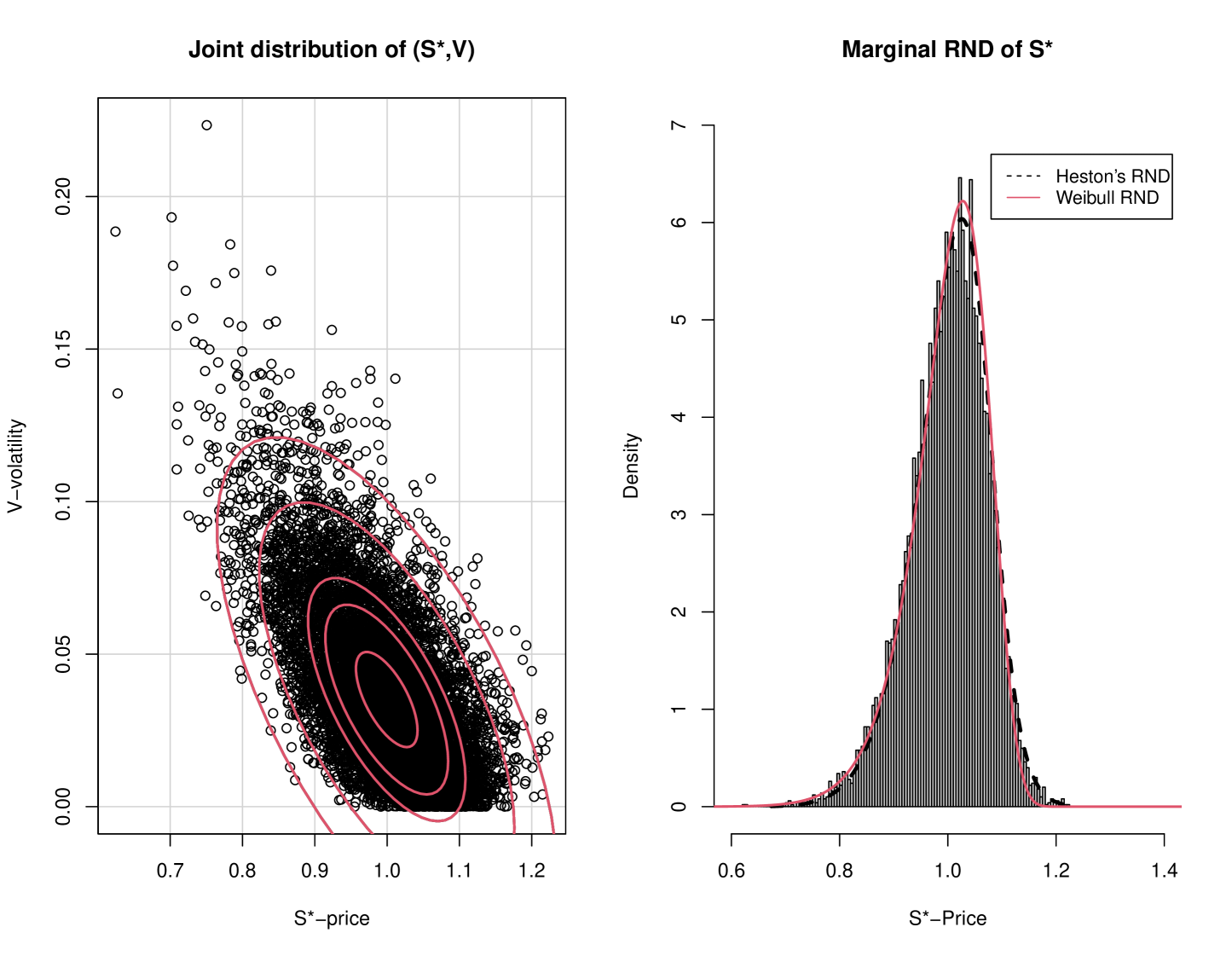
Example: S&P 500: Bakshi, Cao and Chen (1997) presented an extensive market data study for comparing several competing stochastic volatility models, including that of Heston’s (1993). The data used covered options and spot prices for the S&P 500 Index starting from June 1, 1988 through May 31, 1991. From Table III there we find that in addition to , the ‘All Option’ estimated (or implied) structural parameter, corresponding Heston’s SV model, is
In this case, , hence we used Milstein (reflective) scheme to obtain, for a short contract duration with year, a Monte-Carlo sample of simulated pairs with (standardized) spot price and volatility, according to the SV model (1). Their joint distribution is presented in Figure 1a, where we have superimposed the matching 16%, 50%, 68% , 95% and 99.5% contour lines. In Figure 1b we present the histogram of the simulated marginal distribution of the spot price . The mean and standard deviation of these simulated spot price values are and . We also included in the figure the curve of the (implied, by ) Heston’s RND as was computed directly by using (31). As is expected in the case of (risk-neutrality) modeling the spot prices of an Index, the implied RND is negatively skewed () which suggests a comparison against the Weibull distribution of Section 3.4. To that end, (and since we do not have the actual option data used by the authors) we simply matched to the ‘observed’ value of and used it to obtain the numerical solution of equation (24) as at which point, . For comparison, we also added to Figure 1b the plot of the RND. As can be seen, the two RND curves are almost indistinguishable.
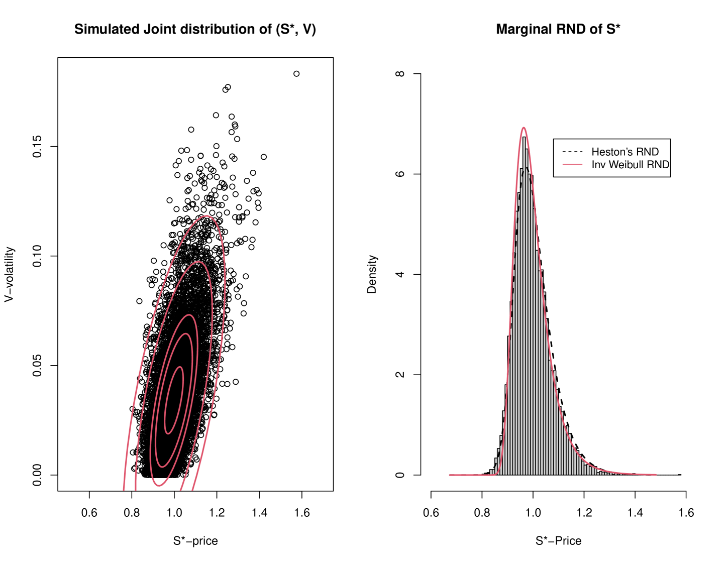
To further illustrate the applicability of the proposed RND to situations with distinct positive Skewness, we considered again Bakshi, Cao and Chen (1997) calibrated parametrization used for Figure 1, but now with a (hypothetically) positive correlation, so that The simulated Monte-Carlo distributions (joint and marginal) are presented in Figure 2, exhibiting the distinct positive Skewness of Heston’s RND (calculated from (31)). This suggested a comparison to the Inverse Weibull distribution discussed in Section 3.5. The mean and standard deviation of these simulated spot price values are and . Again, the value of was match to to obtain the solution of equation (26) as at which point, . Accordingly, we added for comparison, the plot of the RND to Figure 2b, illustrating the extent of the agreement between Heston’s (implied) RND and the Inverse Weibull distribution in this case (with a distinct positives skew).
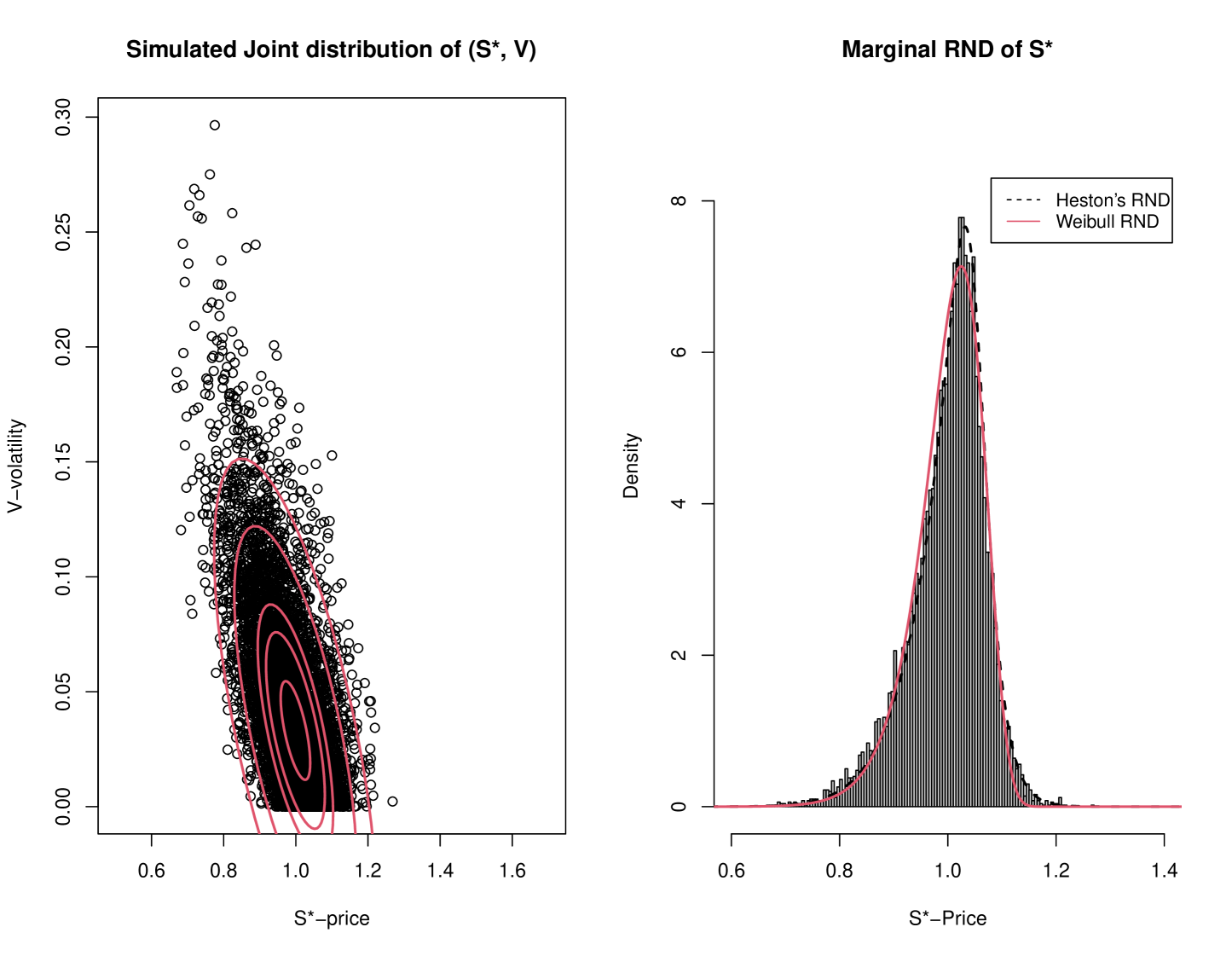
Example: ODAX: Mrázek and Pospíšil (2017) studies various optimization techniques for calibrating and simulating the the Heston model. For demonstrate their results, they used the ODAX option Index with 5 blended maturities of three and six months and with 107 strikes, as were recored on March 19, 2013. The calibrated results of the structural parameter are provided in Table 4 there,
with and with “current” and with . Under this parametrization, we simulated with , a total of pairs of to obtain from the discretized process, the renditions of their joint distribution as well as the marginal distribution of . These are presented in Figure 3. The mean and standard deviation of these simulated spot price values are and . Superimposed, is the Heston’s RND as was calculated, under this parametrization, from the characteristic function given the appendix. Again, as is expected for this index too, the implied RND is negatively skewed () which suggests a comparison against the Weibull distribution. In this case too, the value of was match to to obtain the solution of equation (26) as at which point, . The graph of the Weibull distribution, , is also displayed in the figure, indicating the excellent agreement, in this case two, between the RNDs.
Example: AMD: This example is based on real and current option data that we retrieved from Yahoo Finance as of the closing of trading on December 31, 2020. The closing price of his stock, on that day, was and it pays no dividend, so that to add to the prevailing (risk-free) interest rate of . We chose this stock, AMD (Advanced Micro Devices Inc.) which is a member of the technology sector, since it exhibits more directional risk to the upside, and hence with potentially, positively skewed RND.
From the available option series, we selected the February 19, 2021 expiry, due to the relatively short contract with and some strikes, with corresponding call option (market) prices are available (we actually recorded the option prices as the average between the bid and ask). As standard measure of the goodness-of-fit between the model-calculated option price and the option market price , we used the Mean Squared Error, MSE,
To calibrate the Heston SV model, we used the optim() function of R, to minimize over the model’s parameter , with the initial values of and with . The results of the calibrated values are
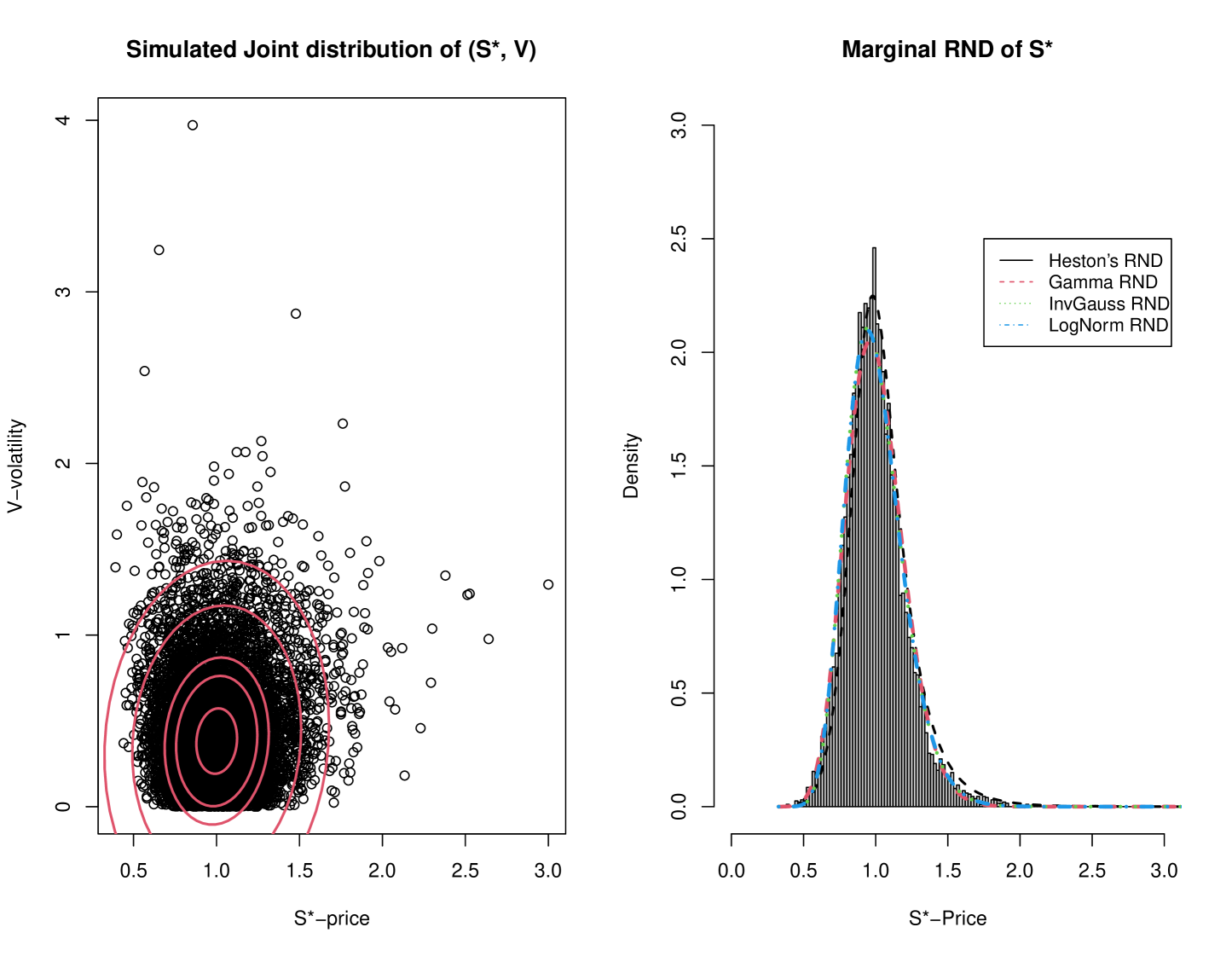
This calibrated parameter, , was then used to calculate, using Heston’s characteristic function, the option prices according to Heston’s SV model (5). These values are displayed in Table 2, along with the actual market prices. Next, we obtained, as in the previous examples, a Monte-Carlo sample of whose results are displayed in Figure 4. The mean and standard deviation of these simulated stock prices are and , respectively. As can be seen, the implied Heston’s RND is, as was expected, positively skewed (). Accordingly, we considered those distribution from Table 1, as possible RND candidates in this situation.
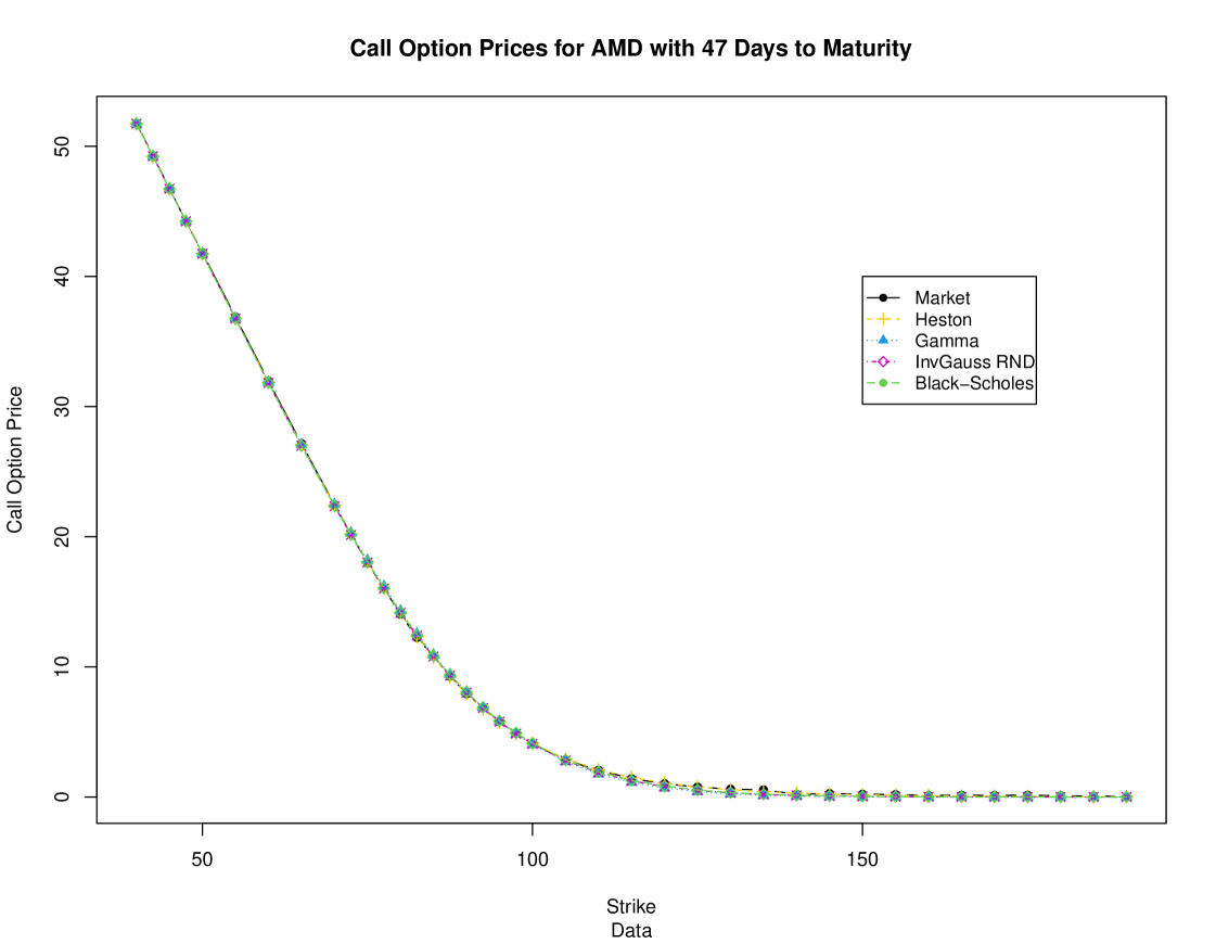
Since in this case, we have available the actual market option prices, we may estimate the parameter , defining these distribution directly, using the ‘standard’ Black-Scholes implied volatility, namely . This entails using the the optim() function again to minimize the with respect to the single parameter . This standard estimation procedure yielded , so that . With this value at hand, we added to Figure 4b the graphs of the Gamma, Inverse Gaussian and the Log-Normal RND, as in Table 1. The extent of their agreement with the Heston’s implied RND is self-evident. To further demonstrate that very point, we calculated the option prices under each one of these modeled RND, and calculated the corresponding . The results of this comparison are presented, side-by-side in Table 2. In Figure 5 we display the option price curve for each of these pricing models– they are ‘virtually’ almost identical in this example.
| MSE | 0.004410 | 0.032725 | 0.018126 | 0.016748 | |
|---|---|---|---|---|---|
| Strike | Market Price | Heston | Gamma | InvGaussan | Black.Scholes |
| 40.0 | 51.775 | 51.720 | 51.738 | 51.737 | 51.737 |
| 42.5 | 49.275 | 49.222 | 49.239 | 49.238 | 49.238 |
| 45.0 | 46.775 | 46.726 | 46.741 | 46.739 | 46.739 |
| 47.5 | 44.200 | 44.231 | 44.244 | 44.240 | 44.240 |
| 50.0 | 41.825 | 41.741 | 41.751 | 41.742 | 41.743 |
| 55.0 | 36.875 | 36.779 | 36.783 | 36.758 | 36.762 |
| 60.0 | 31.950 | 31.869 | 31.871 | 31.816 | 31.824 |
| 65.0 | 27.150 | 27.058 | 27.073 | 26.977 | 26.993 |
| 70.0 | 22.450 | 22.423 | 22.476 | 22.339 | 22.365 |
| 72.5 | 20.200 | 20.203 | 20.285 | 20.132 | 20.164 |
| 75.0 | 17.975 | 18.070 | 18.184 | 18.022 | 18.059 |
| 77.5 | 16.025 | 16.039 | 16.186 | 16.022 | 16.064 |
| 80.0 | 14.050 | 14.127 | 14.302 | 14.145 | 14.190 |
| 82.5 | 12.250 | 12.349 | 12.544 | 12.399 | 12.449 |
| 85.0 | 10.800 | 10.719 | 10.917 | 10.793 | 10.846 |
| 87.5 | 9.275 | 9.242 | 9.428 | 9.330 | 9.385 |
| 90.0 | 7.925 | 7.923 | 8.077 | 8.010 | 8.066 |
| 92.5 | 6.850 | 6.760 | 6.866 | 6.830 | 6.888 |
| 95.0 | 5.800 | 5.746 | 5.790 | 5.786 | 5.843 |
| 97.5 | 4.925 | 4.871 | 4.844 | 4.870 | 4.927 |
| 100.0 | 4.100 | 4.120 | 4.021 | 4.073 | 4.129 |
| 105.0 | 2.835 | 2.939 | 2.706 | 2.799 | 2.852 |
| 110.0 | 2.065 | 2.096 | 1.766 | 1.880 | 1.928 |
| 115.0 | 1.410 | 1.498 | 1.119 | 1.237 | 1.278 |
| 120.0 | 1.025 | 1.075 | 0.688 | 0.798 | 0.833 |
| 125.0 | 0.765 | 0.776 | 0.412 | 0.506 | 0.535 |
| 130.0 | 0.605 | 0.563 | 0.240 | 0.315 | 0.338 |
| 135.0 | 0.550 | 0.411 | 0.136 | 0.194 | 0.211 |
| 140.0 | 0.205 | 0.302 | 0.076 | 0.117 | 0.131 |
| 145.0 | 0.265 | 0.224 | 0.041 | 0.070 | 0.080 |
| 150.0 | 0.215 | 0.167 | 0.022 | 0.042 | 0.049 |
| 155.0 | 0.185 | 0.125 | 0.011 | 0.024 | 0.029 |
| 160.0 | 0.110 | 0.094 | 0.006 | 0.014 | 0.017 |
| 165.0 | 0.135 | 0.072 | 0.003 | 0.008 | 0.010 |
| 170.0 | 0.120 | 0.055 | 0.001 | 0.005 | 0.006 |
| 175.0 | 0.135 | 0.042 | 0.001 | 0.003 | 0.004 |
| 180.0 | 0.095 | 0.032 | 0.000 | 0.001 | 0.002 |
| 185.0 | 0.070 | 0.025 | 0.000 | 0.001 | 0.001 |
| 190.0 | 0.040 | 0.020 | 0.000 | 0.000 | 0.001 |
Source: Yahoo Financial: www.https://finance.yahoo.com/
5 Appendix
Heston (1993) provided (semi) closed form expressions to the probabilities and that comprise the solution in (5) to the option valuation under the stochastic volatility model (1). Starting from a ‘guess’ of the Black-Sholes style solution,
| (27) |
he has shown that with , this solution must satisfy the SDE resulting from the SV model in (1),
for , where and . These closed form expressions are given by
| (28) |
where and is the characteristics function
| (29) |
where is the of corresponding to the probability and
We point out that above is taken to be the positive root of the Riccati equation involving . However using instead the negative root, namely , was shown to provide an equivalent, but yet more stable solution for above -see Albrecher, Mayer, Schoutens, and Tistaer, (2007) for more details on this so-called “Heston Trap”. In either case, efficient numerical routines such as the cfHeston and callHestoncf functions of the NMOF package of R, are readily available to accurately compute the values of and hence of and the call option values, for given and and any choice of .
Now, having established (29), the standard application of the Fourier transform provides (see for example Schmelzle (2010)) that the of , can be obtained, for , as
| (30) |
Hence, it follows immediately that the of is given by
Further, since the characteristic functions in (29) are affine in , where as in Corollary 1, , we may rewrite above as
| (31) |
where
We point out that in light of (8) that in (31) is the RND (under ) for the Heston’s (1993) model and can similarly be easily evaluated numerically along-side of evaluating . Indeed we have,
It should be noticed from expression (31) that any RND, of the Heston Model, and the corresponding risk neutral distribution of , constitutes a scale-family of distributions in , so that it satisfies the terms of Assumption A. This assertion is summarized in Proposition 1 below.
Proposition 1
The result stated in the next claim is known, but the details are instructive to proving (11).
Claim 1
References
- [1] Albrecher, H., Mayer, P., Schoutens, W. and Tistaer, J., (2007). The Little Heston Trap. The Wilmott Magazine, 83–92.
- [2] Alfonsi A., (2010) High order discretization schemes for the CIR process: Application to affine term structure and Heston models. Math. Comp. 79(269), 209–237.
- [3] Andersen L., (2008) Simple and efficient simulation of the Heston stochastic volatility model. J. Comput. Finance, 11(3), 2008, 1–42.
- [4] Black F., and Scholes M., (1973). The pricing of options and corporate liabilities. The Journal of Political Economy, 637-654.
- [5] Bakshi G., Cao C. and Chen Z., (1997) Empirical Performance of Alternative Option Pricing Models. The Journal of Finance, Vol. LII, No. 5, 2003-2049.
- [6] Cox J.C. and Ross S., (1976) The valuation of options for alternative stochastic processes. J. Fin. Econ. 3:145-66.
- [7] Feller W., (1951) Two singular diffusion problems. Ann. Math. 54(1), 173–182.
- [8] Figlewski S., (2010). “Estimating the Implied Risk Neutral Density for the U.S. Market Portfolio”, in Volatility and Time Series Econometrics: Essays in Honor of Robert F. Engle, (eds. Tim Bollerslev, Jeffrey Russell and Mark Watson) Oxford University Press, Oxford, U.K.
- [9] Figlewski S., (2018). Risk Neutral Densities: A Review. Available at SSRNhttp://ssrn.com/abstract=3120028.
- [10] Gatheral, J., (2006). The Volatility Surface, John Wiley and Sons, NJ.
- [11] Grith M. and Krätschmer V., (2012) “Parametric Estimation of Risk Neutral Density Functions”, in: Ed: Duan JC., Härdle W., Gentle J. (eds) Handbook of Computational Finance Springer Handbooks of Computational Statistics. Springer, Berlin, Heidelberg.
- [12] Heston S.L., (1993) A closed-form solution for options with stochastic volatility with applications to bond and currency options. Rev. Financ. Stud. 6(2), 327–343.
- [13] Jackwerth, J. C., (2004). Option-Implied Risk-Neutral Distributions and Risk Aversion Research Foundation of AIMR, Charlotteville, NC
- [14] Jackwerth, J. C. and Rubinstein, M., (1996). Recovering Probability Distributions from Option Prices. The Journal of Finance, 51, no. 5: 1611-631.
- [15] Jiang, L. (2005). Mathematical Modeling and Methods of Option Pricing, Translated from Chinese by Li. C, World Scientific, Singapore.
- [16] Lemaire, V., Montes, T. and Pagès, G., (2020). Stationary Heston model: Calibration and Pricing of exotics using Product Recursive Quantization. Available at arXiv [q-fin.MF]: arXiv:2001.03101v2.
- [17] Merton, R., (1973). Theory of rational option pricing. The Bell Journal of Economics and Management Science, 141-183.
- [18] Mil’shtein, G. N. (1975). Approximate Integration of Stochastic Differential Equations. Theory of Probability & Its Applications, 19 (3), 557–562.
- [19] Mizrach, B. (2010). “Estimating Implied Probabilities from Option Prices and the Underlying” in Handbook of Quantitative Finance and Risk Management (C.-F. Lee A. Lee and J. Lee (eds.)). Springer Science Business Media.
- [20] Mrázek, M. and Pospíšil, J. (2017). Calibration and simulation of Heston model. Open Mathematics— Vol. 15(1), https://doi.org/10.1515/math-2017-0058.
- [21] R Core Team, (2017). R: A Language and Environment for Statistical Computing. Vienna, Austria, https://www.R-project.org/
- [22] Stein J. and Stein E., (1991). Stock price distributions with stochastic volatility: An analytic approach. Rev. Financ. Stud. 4(4), 727–752.
- [23] Schmelzle, M., (2010). Option Pricing Formulae using Fourier Transform: Theory and Application. Technical Report, Available on line at https://pfadintegral.com/articles/option-pricing-formulae-using-fourier-transform/
- [24] Savickas, R., (2002). A simple option formula. The Financial Review, Vol 37, 207-226.
- [25] Savickas, R., (2005). Evidence on delta hedging and implied volatilities for the Black-Scholes, gamma, and Weibull option pricing models. The Journal of Financial Research, Vol 18:2, 299-317.
- [26] Wiggins, B. J., (1987). Option values under stochastic volatility: Theory and empirical estimates. Journal of Financial Economics, Vol. 19(2), 351-372