On the stability of relativistic perfect fluids with linear equations of state where
Abstract.
For , we consider the stability of two distinct families of spatially homogeneous solutions to the relativistic Euler equations with a linear equation of state on exponentially expanding FLRW spacetimes. The two families are distinguished by one being spatially isotropic while the other is not. We establish the future stability of nonlinear perturbations of the non-isotropic family for the full range of parameter values , which improves a previous stability result established by the second author that required to lie in the restricted range . As a first step towards understanding the behaviour of nonlinear perturbations of the isotropic family, we construct numerical solutions to the relativistic Euler equations under a -symmetry assumption. These solutions are generated from initial data at a fixed time that is chosen to be suitably close to the initial data of an isotropic solution. Our numerical results reveal that, for the full parameter range , the density contrast associated to a nonlinear perturbation of an isotropic solution develops steep gradients near a finite number of spatial points where it becomes unbounded at future timelike infinity. This behaviour, anticipated by Rendall in [18], is of particular interest since it is not consistent with the standard picture for inflation in cosmology.
1. Introduction
Relativistic perfect fluids with a linear equation of state on a prescribed spacetime are governed by the relativistic Euler equations111Our indexing conventions are as follows: lower case Latin letters, e.g. , will label spacetime coordinate indices that run from to while upper case Latin letters, e.g. , will label spatial coordinate indices that run from to .
| (1.1) |
where
is the stress energy tensor, is the fluid four-velocity normalized by , and the fluid’s proper energy density and pressure are related by
Since is the square of the sound speed, we will always assume222While this restriction on the sound speed is often taken for granted, it is, strictly speaking, not necessary; see [7] for an extended discussion. that in order to ensure that the speed of sound is less than or equal to the speed of light. We further restrict our attention to exponentially expanding Friedmann-Lemaître-Robertson-Walker (FLRW) spacetimes where and333By introducing a change of time coordinate via , the metric (1.2) can be brought into the more recognizable form , where now .
| (1.2) |
with
| (1.3) |
It is important to note that, due to our conventions, the future is located in the direction of decreasing and future timelike infinity is located at . Consequently, we require that holds in order to guarantee that the four-velocity is future directed. For use below, we find it convenient to introduce the conformal four-velocity via
| (1.4) |
1.1. Stability for
It can be verified by a straightforward calculation that
| (1.5) |
defines a spatially homogeneous solution of the relativistic Euler equations (1.1) on the exponentially expanding FLRW spacetimes for any choice of the parameter and constant . From a cosmological perspective, these solutions are, in a sense, the most natural since they are also spatially isotropic and hence do not determine a preferred direction.
The future, nonlinear stability of the solutions (1.5) on the exponentially expanding FLRW spacetimes was first established in the articles444In these articles, stability was established in the more difficult case where the fluid is coupled to Einstein’s equations. However, the techniques used there also work in the simpler setting considered in this article where gravitational effects are neglected. articles [20, 22] for the parameter values . Stability results for the end points and were established later555Again, stability was established in these articles in the more difficult case where the fluid is coupled to Einstein’s equations. in [13] and [8], respectively. See also [6, 10, 11, 14] for different proofs and perspectives, the articles [9, 12] for related stability results for fluids with nonlinear equations of state on the exponentially expanding FLRW spacetimes, the articles [4, 23, 26] for analogous stability results on other classes of expanding cosmological spacetimes, and [19] for related, early stability results for the Einstein-scalar field system. One of the important aspects of these works is they demonstrate that spacetime expansion can suppress shock formation in fluids, which was first discovered in the Newtonian cosmological setting [25]. This is in stark contrast to fluids on Minkowski space where arbitrary small perturbations of a class of homogeneous solutions to the relativistic Euler equations form shocks in finite time [3].
A consequence of these stability proofs is that the spatial components of the conformal four-velocity of small, nonlinear perturbations of the homogeneous solution (1.5) decay to zero at future timelike infinity, that is,
for the parameter values . This behaviour is, of course, consistent with the isotropic homogeneous solutions (1.5). On the other hand, when , the spatial components of the conformal four-velocity for perturbed solutions do not, in general, decay to zero at timelike infinity, and instead limit to a spatial vector field on , that is,
This behaviour is consistent with a family of non-isotropic homogeneous solutions defined by666More generally, we could set the spatial components of the conformal four-velocity to be any non-zero vector in and determine via the conditions and . However, for simplicity, we will assume here that is chosen so that it is pointing in the direction of the coordinate vector field .
| (1.6) |
where , which satisfy the relativistic Euler equations for . The known stability results for imply the future stability of nonlinear perturbations of these solutions.
Noting that solutions of the type (1.6) can be made arbitrarily close to solutions of the type (1.5) for by choosing sufficiently small, from a stability point of view there seems to be verify little difference between the two classes of solutions for small . Indeed, the future nonlinear stability of both classes of solutions, where is sufficiently small, can be achieved via a common proof. However, as will become clear, the essential difference between these solutions is that, from an initial data point of view, stable perturbations of solutions of the type (1.5) are generated from initial that is sufficiently close to and satisfies
| (1.7) |
while stable perturbations of solutions of the type (1.6) are generated from initial data that is sufficiently close to and satisfies
| (1.8) |
1.2. Stability for
Until recently, it was not known if any solutions of the relativistic Euler equations were stable to the future for the parameter values . In fact, it was widely believed that solutions to the relativistic Euler were not stable for these parameter values. This belief was due, in part, to the influential work of Rendall [18] who used formal expansion to investigate the asymptotic behaviour of relativistic fluids on exponentially expanding FLRW spacetimes with a linear equation of state. Rendall observed that the formal expansions become inconsistent for in the range if the leading order term in the expansion of at vanished somewhere. He speculated that the inconsistent behaviour is the expansions could be due inhomogeneous features developing in the fluid density that would ultimately result in the blow-up of the density contrast at future timelike infinity. Speck [23, §1.2.3] added further support to Rendall’s arguments by presenting a heuristic analysis that suggested uninhibited growth would set in for solutions of the relativistic Euler equations for the parameter values . Combined, these considerations left the stability of solutions to the relativistic Euler equations in doubt for in the range .
However, it was established in [16] that there exists a class of non-isotropic homogeneous solutions of the relativistic Euler equations that are stable to the future under small, nonlinear perturbations. This class of homogeneous solutions should be viewed as the natural continuation of the solutions (1.6) over the parameter range , and they are defined by
| (1.9) |
where
| (1.10) |
and solves the initial value problem (IVP)
| (1.11) | ||||
| (1.12) |
Existence of solutions to this IVP is guaranteed by Proposition 3.1. from [16], which we restate here:
Proposition 1.1.
The main result of [16] was a proof of the nonlinear stability to the future of the homogeneous solutions (1.9) for the parameter values . It was also established in [16] that under a -symmetry assumption, future stability held for the full parameter range . An important point that is worth emphasising is that the initial data used to generate the perturbed solutions from [16] satisfies the condition (1.8) at , and furthermore, this positivity property propagates to the future in the sense that the perturbed solutions satisfy
It is this property of the perturbed solutions from [16] that avoids the problematic scenario identified by Rendall.
This article has two main aims: the first is to establish the nonlinear stability to the future of the homogeneous solutions (1.9) for the full parameter range without the -symmetry that was required in [16]. The second aim is to provide convincing numerical evidence that shows the density contrast blow-up scenario of Rendall is realized if the condition (1.8) on the initial data is violated.
Before stating a precise version of our stability result for the homogeneous solutions (1.9), we first recall two formulations of the relativistic Euler equations from [16]. The first formulation, which was introduced in [15] and subsequently employed in [14] to establish stability for the parameter range , involves representing the fluid in terms of the modified fluid density defined via
| (1.14) |
and the spatial components of the conformal fluid four-covelocity777Here and in the following, all spacetime indices will be raised and lowered with the conformal metric . . In terms of these variables, the relativistic Euler equations (1.1) can be formulated as the following symmetric hyperbolic system:
| (1.15) |
where
| (1.16) | ||||
| (1.17) | ||||
| (1.18) | ||||
| (1.19) | ||||
| (1.20) | ||||
| (1.21) | ||||
| (1.22) | ||||
| (1.23) | ||||
| and | ||||
| (1.24) | ||||
The second formulation of the relativistic Euler equations is obtained by introducing a new density variable via
| (1.25) |
and decomposing the spatial components of the conformal fluid four-velocity as
| (1.26) | ||||
| (1.27) | ||||
| and | ||||
| (1.28) | ||||
where solves the IVP (1.11)-(1.12). Then setting
| (1.29) | ||||
| (1.30) | ||||
| (1.31) | ||||
| (1.32) | ||||
| (1.33) | ||||
| and | ||||
| (1.34) | ||||
it was shown in [16, §3.2] that in terms of the variables
| (1.35) |
the relativistic Euler equations become
| (1.36) |
where
| (1.37) |
| (1.38) |
| (1.39) |
| (1.40) |
and
| (1.41) |
For later use, we also define
| (1.42) |
and observe that and satisfy the relations
| (1.43) |
An important point regarding the formulation (1.36) is that it is symmetrizable. Indeed, as shown in [16], multiplying (1.36) by the positive definite, symmetric matrix
| (1.44) |
yields
| (1.45) |
where it is straightforward to verify from (1.37)-(1.39) that the matrices
| (1.46) |
are symmetric, that is,
| (1.47) |
We are now in a position to state the main stability theorem of this article. The proof is presented in Section 2. Before stating the theorem, it is important to note that, due to change of variables defined via (1.25)-(1.28) and (1.35), the homogeneous solutions (1.9) correspond to the trivial solution of (1.36).
Theorem 1.2.
Suppose , , , , , is the unique solution to the IVP (1.11)-(1.12) from Proposition 1.1 and . Then for small enough, there exists a unique solution
to the initial value problem
| (1.48) | ||||
| (1.49) |
provided that
Moreover,
-
(i)
satisfies the energy estimate
for all where888The norm is defined by .
-
(ii)
there exists functions and such that the estimate
holds for all where
-
(iii)
and determine a unique solution of the relativistic Euler equations (1.1) on the spacetime region via the formulas
(1.50) (1.51) (1.52) (1.53) (1.54) -
(iv)
and the density contrast satisfies
(1.55)
1.3. Instability for
It is essential for the stability result stated in Theorem 1.2 to hold that the initial data used to generated the nonlinear perturbations of homogeneous solutions of the type (1.9) satisfies the condition (1.8). This leaves the question of what happens when this condition is violated, which would be guaranteed to happen for some choice of initial data from any given open set of initial data that contains initial data corresponding to an isotropic homogeneous solution (1.5). To investigate this situation, we consider a -symmetric reduction of the system (1.15) obtained by the ansatz
| (1.56) | ||||
| (1.57) |
where is as defined above by (1.25). It is not difficult to verify via a straightforward calculation that the relativistic Euler equations (1.15) will be satisfied provided that and solve999Here, we set .
| (1.58) | ||||
| (1.59) |
In Section 3, we numerically solve this system for specific choices of initial data
Importantly, these choices include initial data for which crosses zero at two points in , and as a consequence, violates the condition (1.8). From our numerical solutions, we observe the following behaviour:
- (1)
-
(2)
For each and each choice of initial data that violates (1.8) and is sufficiently close to homogeneous initial data of the family of solutions (1.5), there exists a such that
This indicates an instability in the -spaces for solutions of (1.58)-(1.59) that is not present, c.f. Theorem 1.2, in solutions generated from initial data satisfying (1.8). We also observe that the integer is a monotonically decreasing function of with a minimum value of . For the initial data we tested, the blow-up at in the derivatives occurs at a finite set of spatial points.
-
(3)
For all and all choices of initial data that are sufficiently close to homogeneous initial data of either family of solutions (1.5) and (1.9), solutions to (1.58)-(1.59) are approximated remarkably well, for times sufficiently close to zero, by solutions to the asymptotic system101010Note this system is obtain from (1.58)-(1.59) simply by discarding the terms involving spatial derivatives.
(1.60) (1.61) everywhere except, possibly, at a finite set of points where steep gradients form in , which only happens for large enough and initial data violating (1.8).
-
(4)
For each and each choice of initial data that violates (1.8) and is sufficiently close to homogeneous initial data of the family of solutions (1.5), the density contrast develops steep gradients near a finite number of spatial points where it becomes unbounded as . This behaviour was anticipated by Rendall in [18], and it is not consistent with either the standard picture for inflation in cosmology where the density contrast remains bounded as , or with the behaviour of the density contrast of solutions generated from initial data satisfying (1.8), c.f. Theorem 1.2.
1.4. Stability/instability for
When the sound speed is equal to the speed of light, i.e. , it is well known that the irrotational relativistic Euler equations coincide, under a change of variables, with the linear wave equation. Even though the future global existence of solutions to linear wave equations on exponentially expanding FLRW spacetimes can be inferred from standard existence results for linear wave equations, a corresponding future global existence result for the irrotational relativistic Euler equations does not automatically follow. This is because the change of variables needed to interpret a wave solution as a solution of the relativistic Euler equations requires the gradient of the wave solution to be timelike. Thus an instability in the irrotational relativistic Euler equations can still occur for if the gradient of the wave solution starts out timelike but becomes spacelike somewhere in finite time. This phenomena was shown in [5] to occur in the more difficult case where coupling to Einstein’s equations with a positive cosmological constant was taken into account. In fact, it was shown in [5] that all wave solutions generated from initial data sets that correspond to a sufficiently small perturbation of the FLRW fluid solution (i.e. (1.5) in our setting) become spacelike in finite time. This proves that the self-gravitating version of the isotropic homogeneous (1.5) are unstable, and in the irrotational setting at least, characterizes the cause of the instability. What is not known is if the other family of homogeneous solutions (1.9) or their self-gravitating versions remain stable for .
1.5. Future directions
The most natural and physically relevant generalization of the the stability result stated in Theorem 1.2 would be an analogous stability result for the coupled Einstein-Euler equations with a positive cosmological constant for satisfying . We expect that establishing this type of stability result is feasible by adapting the arguments from [14]. This expectation is due to the behaviour of the term , which is the only potentially problematic term that could, if it grew too quickly as , prevent the use of the arguments from [14]. However, by Theorem 1.2, we know that and from which it follows that . This shows that decays quickly enough as to expect that it should not be problematic. We are currently working on generalizing Theorem 1.2 to include coupling to Einstein’s equations with a positive cosmological constant, and we will report on any progress in this direction in a follow-up article. We are also planning to investigate numerically, under a Gowdy symmetry assumption, if a similar behaviour, as described in Section 3, occurs for initial data that violates (1.8) when coupling to Einstein’s equations with a positive cosmological constant is taken into account.
2. Proof of Theorem 1.2
2.1. Step 1: Fuchsian formulation
Applying the projection operator to (1.36), while noting that by (1.40)-(1.41), yields
Multiplying this equation through by gives
| (2.1) |
Applying to (1.36), we further observe, with the help of (1.43), that
| (2.2) |
Next, we decompose the term in (2.2) as follows
Inserting this into (2.2) and multiplying the resulting equation on the left by gives
| (2.3) |
It is worth noting at this point that it is the use of this equation to control instead of (2.2) that is responsible for the improvement of the range of the parameter values for which stability holds from in [16] to in this article.
Now, multiplying (2.3) by
| (2.4) |
and adding the resulting equation to (2.1) yields
Setting
| (2.5) |
it is then not difficult to verify that the above equation can be expressed as
| (2.6) |
where
| (2.7) |
Noting from (1.37)-(1.39) that
where
| (2.8) |
a short calculation using (1.41)-(1.42), (1.44), and (2.4) shows that the matrices (2.7) are given by
| (2.9) |
and
| (2.10) |
From these formulas, it is clear that the matrices are symmetric, that is,
| (2.11) |
We proceed by differentiating (1.36) spatially to get
Setting
| (2.12) |
we can write this as
Multiplying the above equation on the left by and recalling the definitions (1.46), we find that satisfies
| (2.13) |
Finally, combining (2.6) and (2.13) yields the Fuchsian system
| (2.14) |
where
| (2.15) | ||||
| (2.16) | ||||
| (2.17) | ||||
| (2.18) | ||||
| and | ||||
| (2.19) | ||||
As will be established in Step 2 below, the Fuchsian system (2.14) satisfies assumption needed to apply the Fuchsian global existence theory from [2]; see, in particular, [2, Thm. 3.8.] and [2, §3.4.]. This global existence theory will be used in Step 3 of the proof to establish uniform bounds on solutions to the initial value problem (1.48)-(1.49) under a suitable small initial data assumption. These bounds in conjunction with a continuation principle will then yield the existence solutions to (1.48)-(1.49) on as well as decay estimates as .
2.2. Step 2: Verification of the coefficient assumptions
In order to apply Theorem 3.8. from [2], see also [2, §3.4.], to the Fuchsian system (2.14), we need to verify that the coefficients of this equations satisfy the assumptions from Section 3.4. of [2], see also [2, §3.1.]. To begin the verification, we set
| (2.20) |
and observe from (1.29)-(1.32), (1.44), (2.9) and (2.16) that the matrix can be treated as a map depending on the variables (2.20), that is,
| (2.21) |
where for each there exists constants such that is smooth on the domain defined by
| (2.22) |
and satisfies
| (2.23) |
for all . In the following, we will always be able to choose and as needed in order to guarantee that the statements we make are valid.
Differentiating with respect to then shows, with the help of (1.29), (2.5) and (2.20)-(2.21), that
| (2.24) |
where
and can be computed from from (2.6), that is,
| (2.25) |
We note from (1.29)-(1.31), (2.4), (2.9) and (2.20) that the matrices
| (2.26) |
are smooth on the domain , and that is bounded below by
| (2.27) |
for all where can be taken as the same constant as in (2.23). We further note from (1.29)-(1.32), (1.44), (1.46), (2.10), (2.8) and (2.20) that the matrices
| (2.28) |
are smooth on the domain (2.22), while is clear from (1.40) that the vector-valued map
| (2.29) |
is smooth on the domain .
Next, setting
| (2.30) |
it follows from (1.29)-(1.34), (1.37)-(1.39) and (2.20) that the matrices can be expanded as
| (2.31) |
where the , are smooth on the domain (2.22) and the are smooth on the domain defined by
It is also not difficult to verify from (1.37)-(1.39) that the satisfy
| (2.32) |
Differentiating the matrices spatially, we have by (1.29), (2.12), (2.20), (2.30) and (2.31) that
| (2.33) |
where
By (1.41)-(1.42) and (1.44), we note that the matrix satisfies and . Using these identities, it is then follows from the definitions (2.16) and (2.18) that satisfies
| (2.34) |
and
| (2.35) |
where
| (2.36) |
Additionally, by (1.41)-(1.43), we observe that satisfies
| (2.37) |
while the symmetry of the matrices , that is,
| (2.38) |
is obvious from the definitions (1.44) and (2.16)-(2.17), and the relations (1.47) and (2.11).
Now, from the definitions (1.29), (2.5), (2.12), (2.15), (2.20) and (2.30), the formulas (2.24) and (2.25), the estimates (1.13) for and , the smoothness properties (2.21), (2.26), (2.28), (2.29) and (2.31) of the matrices , , , , , , and the source term , the lower bound (2.27) on , and the identity (2.32), it is not difficult to verify that for each that there exists a constant such that
| (2.39) |
for all , where . From (2.19) and similar considerations, it is also not difficult to verify
| (2.40) |
for all . It is also clear that we can view (2.14) as an equation for the variables , with and , where the maps and depend on the variables and , respectively.
Taken together, (i) the variable definitions (1.29), (2.5), (2.12), (2.20) and (2.30), (ii) the smoothness properties (2.21), (2.26), (2.28), (2.29) and (2.31) of the matrices , , , , , , and the source term , (iii) the identities (2.34)-(2.35) and the lower bound (2.23) satisfied by matrix , (iv) the definitions (2.17) and (2.19) of the matrices and the source term , (v) the properties (2.37) of the projection map , and (vi) the bounds (2.39) and (2.40) on and , respectively, imply that for any111111By (1.10), corresponds to . and chosen sufficiently small, there exist constants such that the Fuchsian system (2.14) satisfies satisfies all the assumptions from Section 3.4 of [2] for following choice of constants: , , ,
and . As discussed in [2, §3.4], under the time transformation121212Note that our time variable is assumed to be positive as opposed to [2], where it is taken to be negative. This causes no difficulties as we can change between these two conventions by using the simple time transformation . , the transformed version of (2.14) will satisfy all of the assumptions from Section 3.1 of [2]. Moreover, since the matrices have a regular limit as , the constants and from Theorem 3.8 of [2] vanish. This fact together with and implies that the constant131313This constant is denoted by in the article [2]. We denote it here by because is already being used denote the modified density. from Theorem 3.8 of [2] that determines the decay rate is given by .
2.3. Step 3: Existence and uniqueness
By (1.44) and (1.47), we know that the matrices are symmetric. Furthermore, from the analysis carried out in Step 2 above, we know that the matrices and the source term depend smoothly on the variables for and in an open neighbourhood of zero, and that the matrix is positive definite on this neighbourhood. As a consequence, the system (1.48) is symmetrizable and can be put in the symmetric hyperbolic form (1.45) by multiplying it on the left by the matrix . Since and , we obtain from an application of standard local-in-time existence and uniqueness theorems and the continuation principle for symmetric hyperbolic systems, see Propositions 1.4, 1.5 and 2.1 from [24, Ch. 16], the existence of a unique solution
to IVP (1.48)-(1.49) where is the maximal time of existence. From the computations carried out in Step 1 of the proof, this solution determines via (2.5) and (2.12) a solution
| (2.41) |
of the IVP
| (2.42) | ||||
| (2.43) |
where we observe that
| (2.44) |
On the other hand, by Step 2 we can apply141414It it is important to note that the regularity of the initial data (2.44) is less than what is required to apply Theorem 3.8. [2] to the Fuchsian system (2.14). The reason that we can still apply this theorem is that the matrices in (2.14) do not have any singular terms; see Remark A.3.(ii) from [1]. Theorem 3.8. from [2] to the time transformed version of (2.14) as described in [2, Section 3.4] to deduce, for chosen small enough and the initial data satisfying (2.44), the existence of a unique solution
to the IVP (2.42)-(2.43) with that satisfies the following properties:
-
(1)
The limit of as , denoted , exists in .
-
(2)
The solution is bounded by the energy estimate
(2.45) for all , where the implied constant depends on .
-
(3)
For any given , the solution satisfies the decay estimate
(2.46) for all , where the implied constants depend on and .
By uniqueness, the two solutions and to the IVP (2.42)-(2.43) must coincide on their common domain of definition, and consequently, for all . But this implies by (2.41), the energy estimate (2.45), and Sobolev’s inequality [17, Thm. 6.2.1] that
By shrinking if necessary, we can, by (2.44), make as small as we like, which in turn, implies via the above estimate that we can bound by for all , where is as determined in Step 2 of the proof. This bound is sufficient to guarantee that the matrices and the source term from the symmetric hyperbolic system (1.45) remain well defined and that the matrix continues to be positive definite. By the continuation principle and the maximality of , we deduce that , and hence that for all . From this and the energy estimate (2.45), it then follows with the help of the definitions (1.41)-(1.42), (2.5), (2.12), (2.18) and (2.41) that
where
We further obtain from the decay estimate (2.46) and (2.36) the existence of functions and such that
| (2.47) |
for all where
We also note by (1.4), (1.14), (1.17) and (1.25)-(1.28) that and determine a solution of the relativistic Euler equations (1.1) on the spacetime region via the formulas (1.50)-(1.54).
To complete the proof, we find from differentiating (1.50) that the density contrast can be expressed as
| (2.48) |
Since , we can choose small enough so that . Doing so then implies by (2.47) that and converge in to and as . Since converges as well by Proposition 1.1, it is then not difficult to verify from (2.48) and the Sobolev and Moser inequalities [17, Thms. 6.2.1 & 6.4.1] that
which completes the proof.
3. Numerical solutions
3.1. Numerical setup
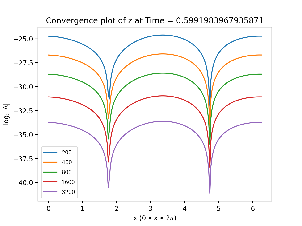
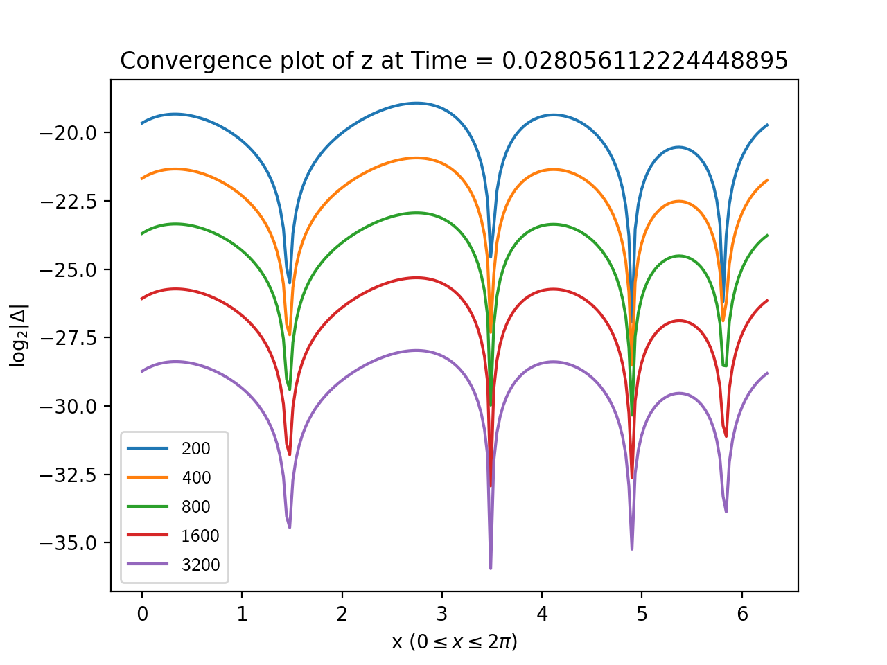
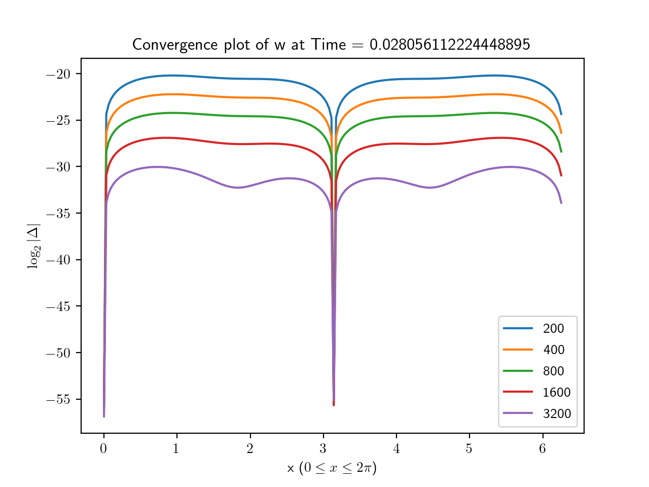
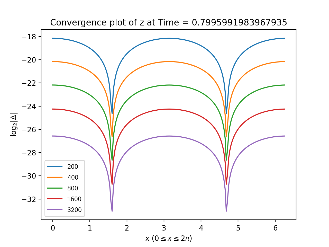
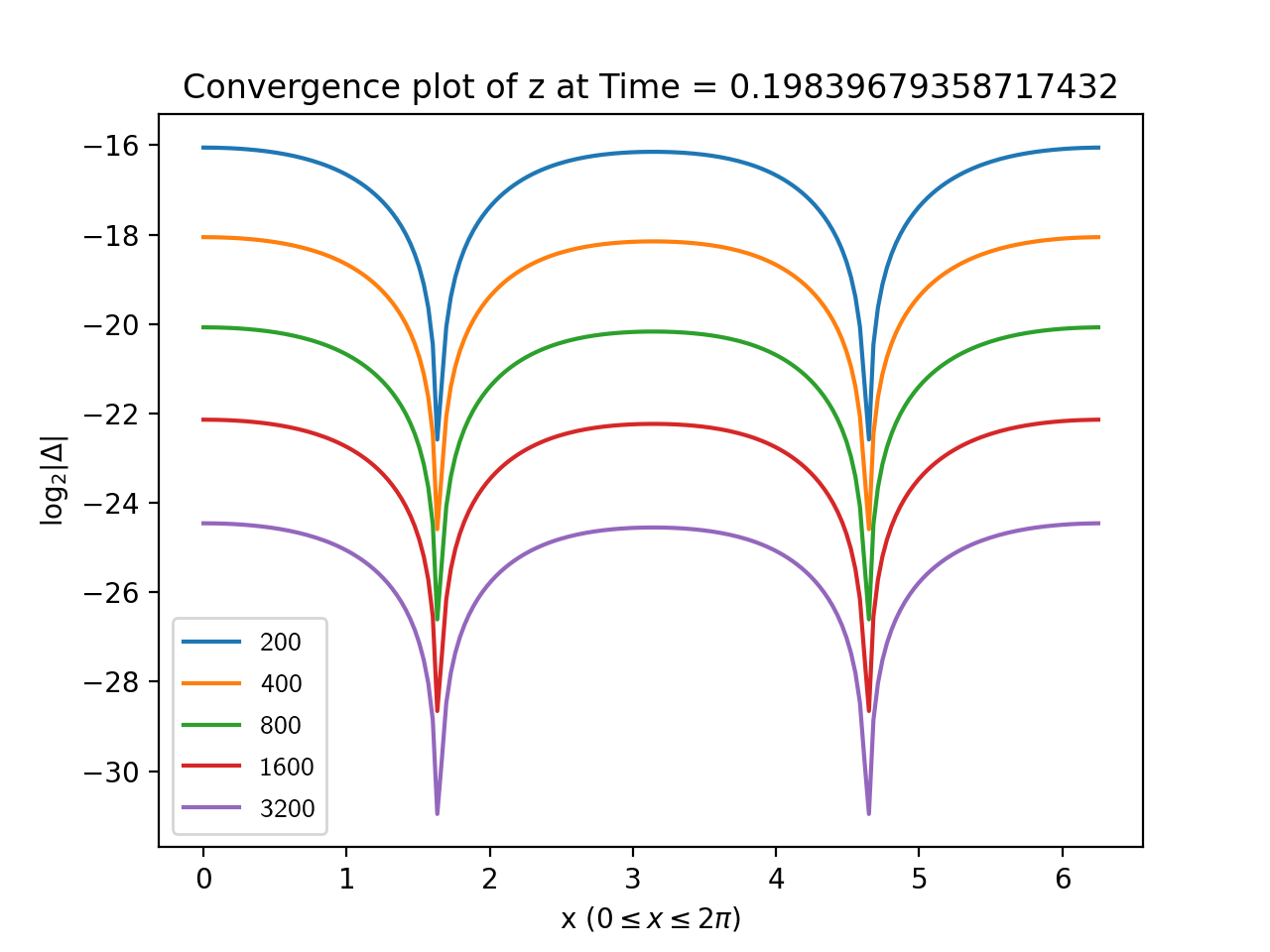
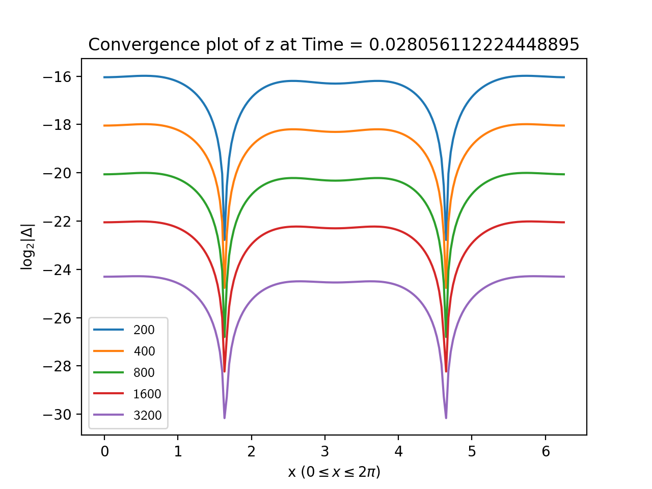
In the numerical setup that we use to solve the system (1.58)-(1.59), the computational domain is with periodic boundary condition, the variables z and w are discretised in space using order central finite differences, and time integration is performed using a standard order Runge-Kutta method (Heun’s Method). As a consequence, our code is second order accurate151515Strictly speaking one also needs to enforce the CFL condition to ensure convergence. In this case we have used the tightened 4/3 CFL condition for Heun’s Method which is discussed in [21]..
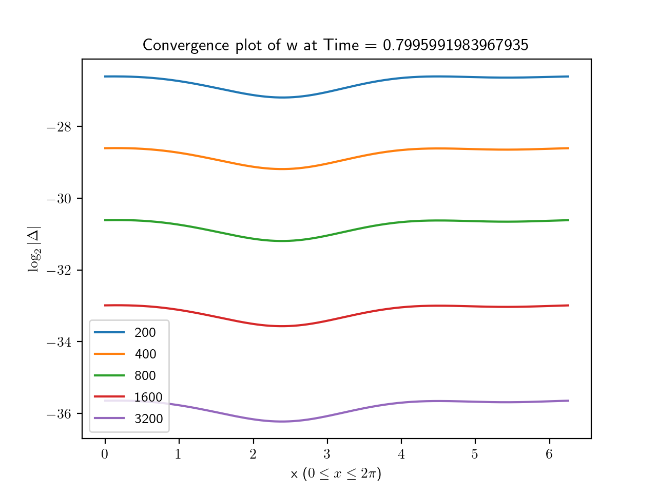
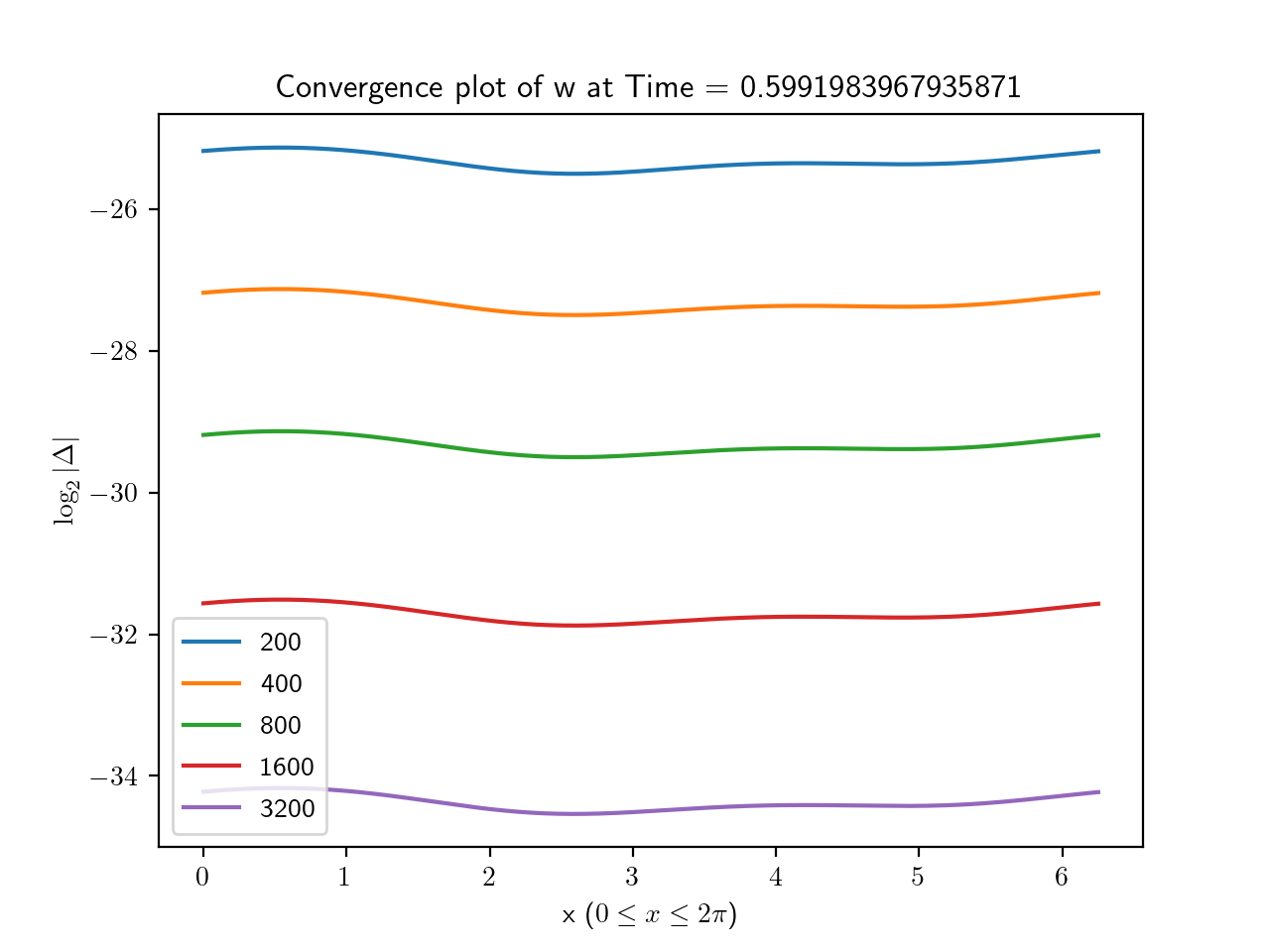
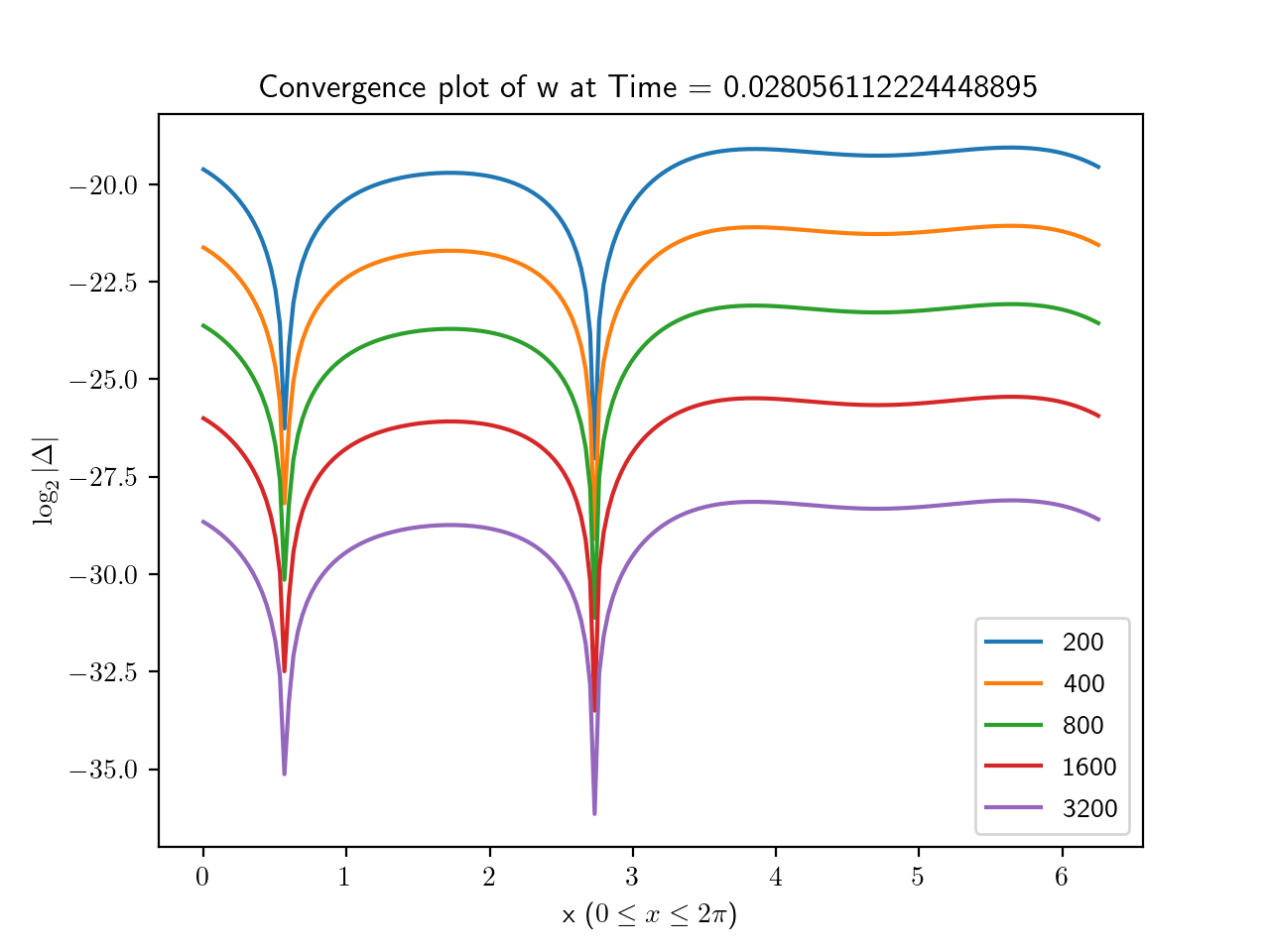
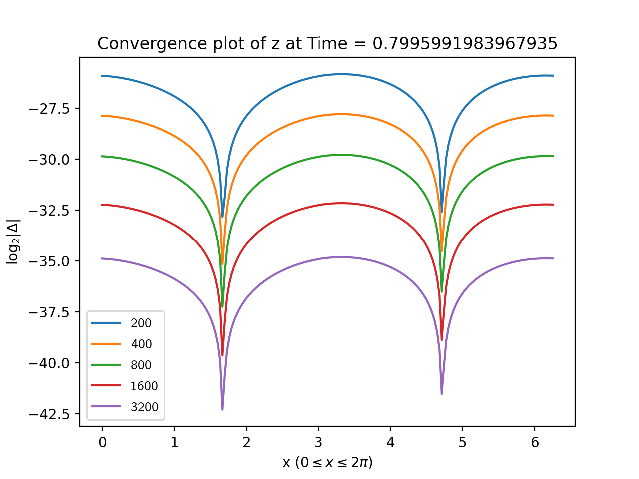
3.1.1. Convergence tests
We have verified the second order accuracy of our code with convergence tests involving perturbations of both types of homogeneous solutions (1.5) and (1.9). In our convergence tests, we have evolved the system (1.58)-(1.59) staring from the the two initial data sets
| (3.1) | ||||
| and | ||||
| (3.2) | ||||
using resolutions of , , , , , and grid points. The initial data (3.1) and (3.2) satisfy the conditions (1.7) and (1.8), respectively, and the solutions generated from this initial data represent perturbations of the homogeneous solutions (1.5) and (1.9), respectively.
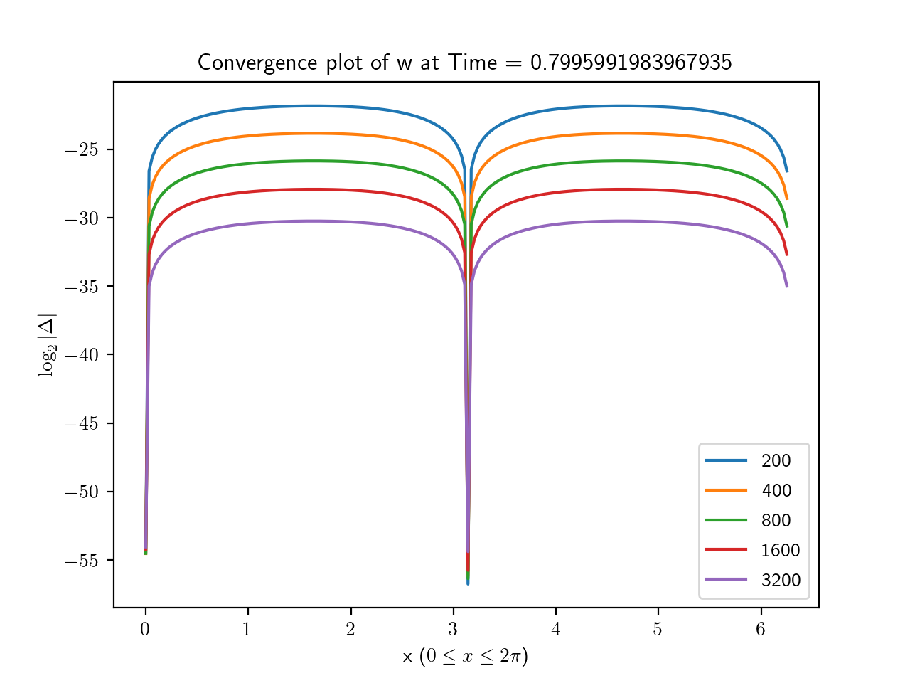
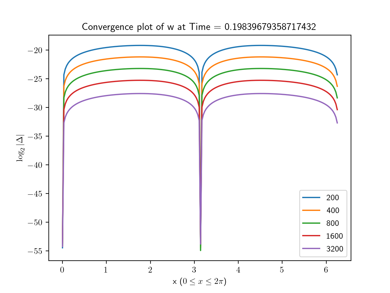
To estimate the error, we took the base 2 log of the absolute value of the difference between each simulation and the highest resolution run. The results for are shown in Figures 1, 2, 3 and, 4 from which the second order convergence is clear.
3.1.2. Code validation
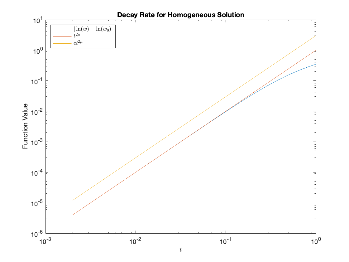
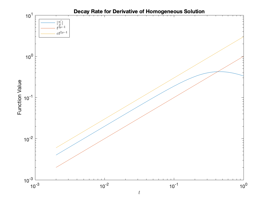
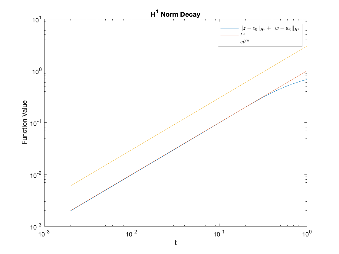
A simple way to test the validity of our code is to verify that numerical solutions to (1.58)-(1.59) that are generated from initial data with satisfy the decay rates of Proposition 1.1
| (3.3) |
and Theorem 1.2
| (3.4) |
We first note that, by equating (1.26) and (1.57) and recalling that for homogeneous solutions, can be expressed in terms of a homogeneous solution of (1.58)-(1.59) as . The decay rates for the homogeneous solution (3.3) can then be re-written in terms of as
| (3.5) | ||||
| (3.6) |
Similarly, for non-homogeneous solutions, we can express in terms of by setting and equating (1.26) and (1.57) to get . The decay rate (3.4), in the norm, is then
| (3.7) |
We have estimated by taking the values of the functions at a time-step close to and calculated using second order central finite differences. As shown in Figure 5, the numerical solutions clearly replicate the above decay rates suggesting the code is correctly implemented.
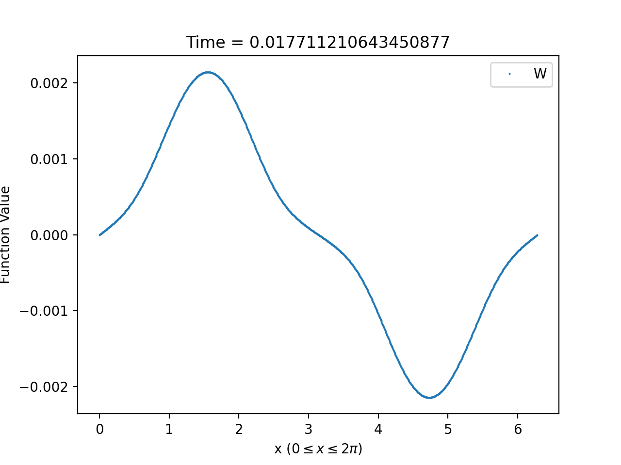
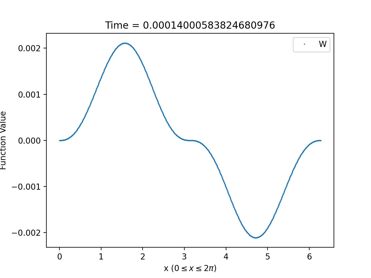
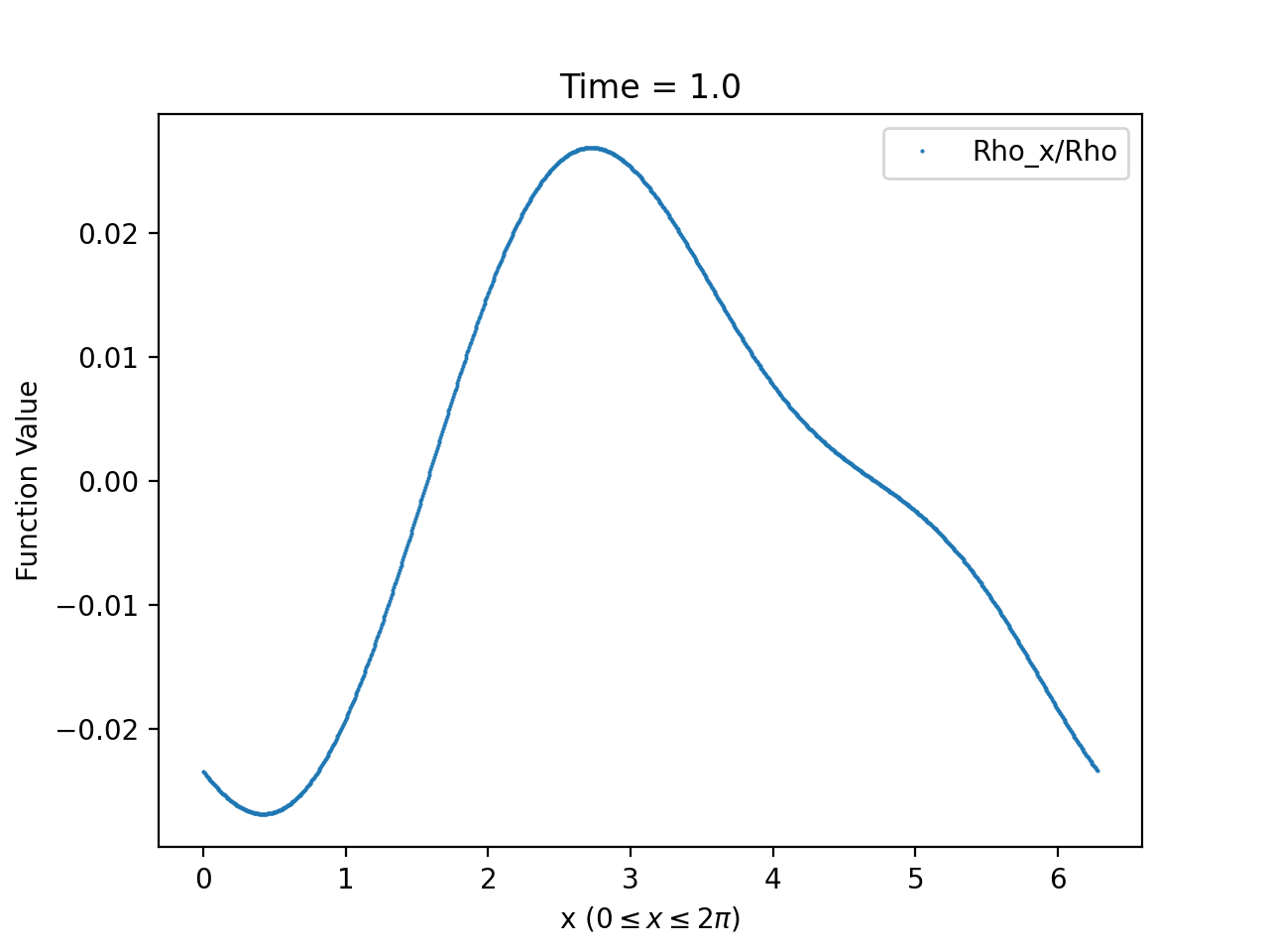
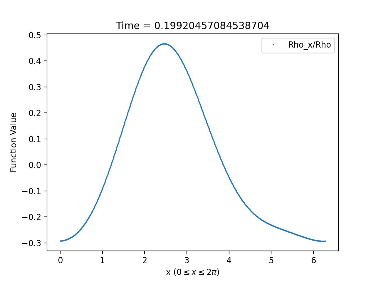
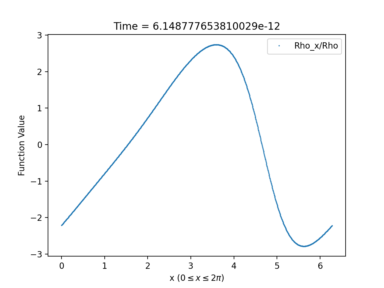
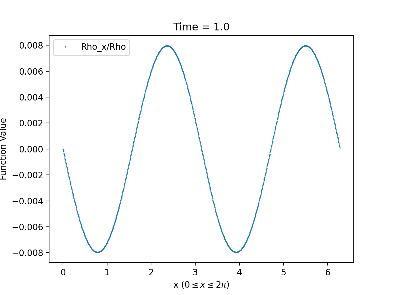
3.2. Numerical behaviour
Beyond the convergence tests, we have generated numerical solutions to the system (1.58)-(1.59) from a variety of initial data sets for which satisfies the conditions (1.7) and (1.8). We employed resolutions ranging from 1000 to 160,000 grid points in our simulations. For initial data satisfying (1.7), we chose functions that cross the -axis at least twice,161616It is necessary to cross the -axis at least twice to enforce the periodic boundary condition. while for initial data satisfying (1.8), does not cross the -axis at all.
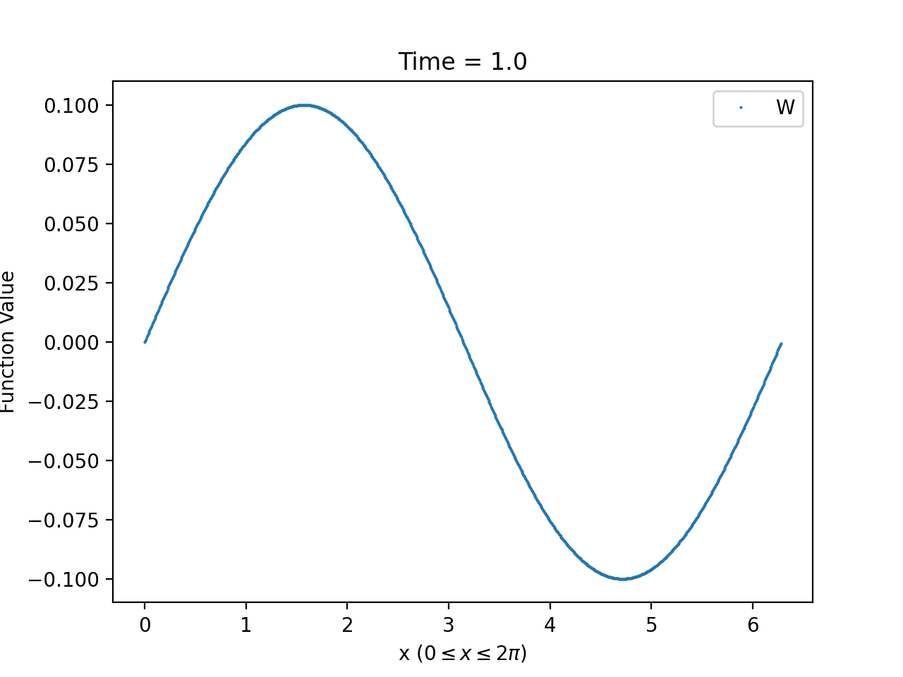
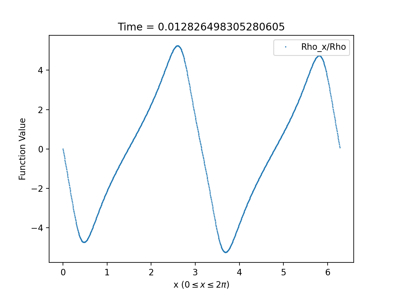
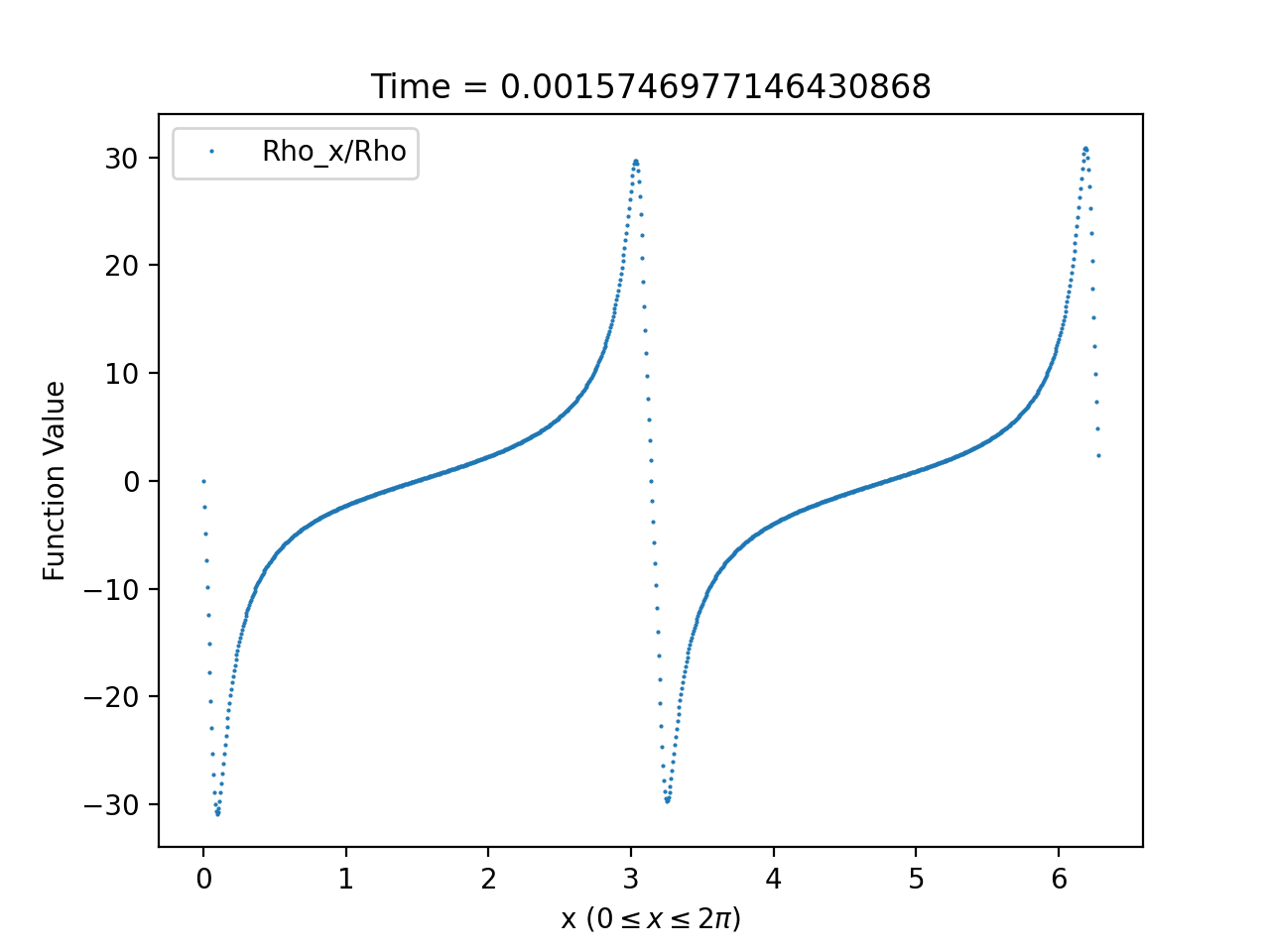
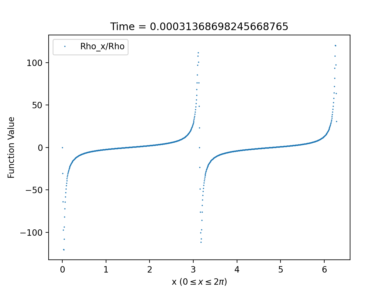
All of the solutions in this article displayed in the figures are generated from initial data of the form
for some particular choice of the constants . From our numerical solutions, we observe, for the full parameter range and all choices of the initial data with sufficiently small, that and remain bounded and converge pointwise as ; see Figures 6 and 7.
3.2.1. Derivative blow-up at
While and remain bounded, our numerical simulations reveal that derivatives of the solutions of sufficiently high order blow-up at for the parameter values and initial data satisfying (1.7). In Table 1, we list, for a selection of values, the corresponding minimum value of for which as . From these values, it appears that is a monotonically decreasing function of .
3.2.2. Asymptotic behaviour and approximations
For the full range of parameter and all choices of initial data, we observe that our numerical solutions display ODE-like behaviour near . In particular, these solutions can be approximated by solutions of the asymptotic system (1.60)-(1.61) at late times using the following procedure:
- (i)
-
(ii)
Fix a time when the numerical solution first appears to be dominated by ODE behaviour.
- (iii)
- (iv)
-
(v)
Compare the numerical solution to the asymptotic solution on the region .
Using this procedure, we find that numerical solutions of the system (1.60)-(1.61) can be remarkably well-approximated by solutions of the asymptotic system. In particular, by setting in (3.9) and noting that we can solve for to get
| (3.10) |
where is the sign function, we have, with the help of (3.8), that
| (3.11) |
It is worth noting that this ODE-like asymptotic behaviour of solutions generated from initial data satisfying (1.8) is expected by Theorem 1.2. What is interesting is that this behaviour of solutions persists for initial data that violates (1.8).
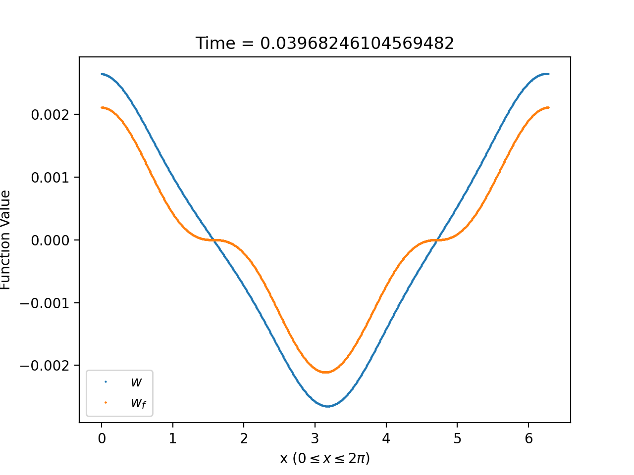
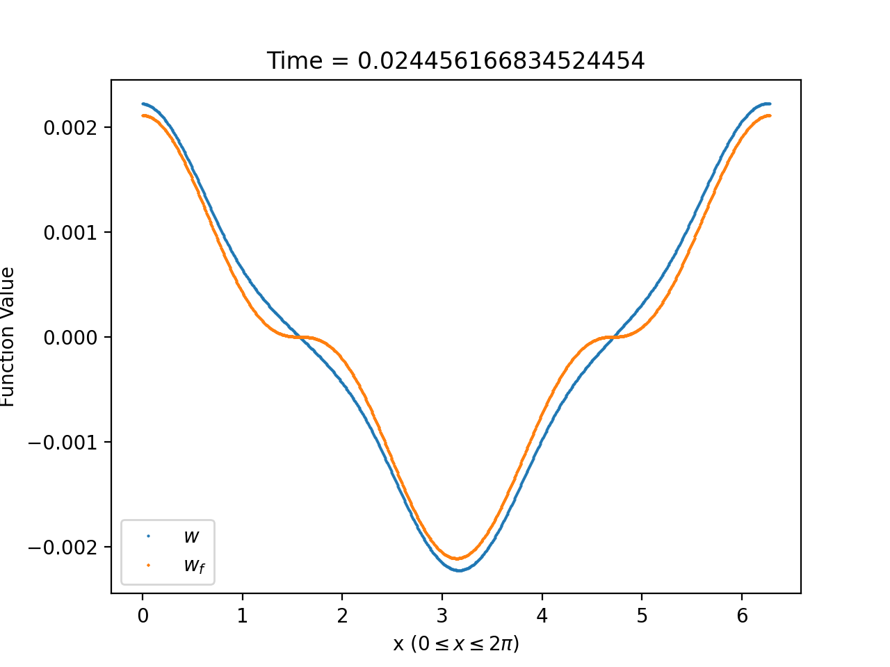
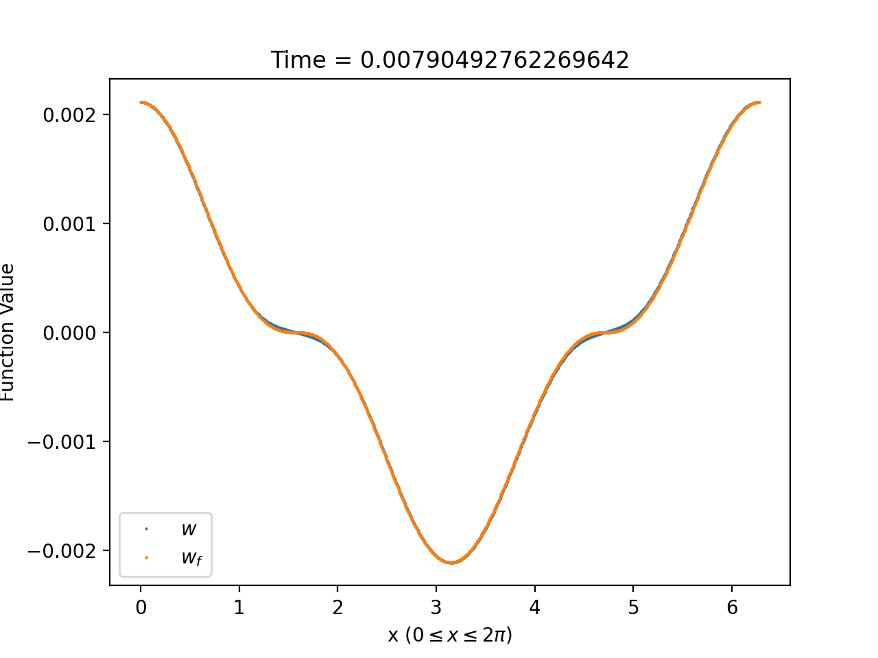
To illustrate how well solutions of (1.58)-(1.59) can be approximated by solutions of the asymptotic system (1.60)-(1.61) near , we compare in Figure 8 the plot of , for a fixed choice of and (see (3.10)), with that of at times close to zero. From the figure, it is clear that the agreement is almost perfect for times close enough to zero.
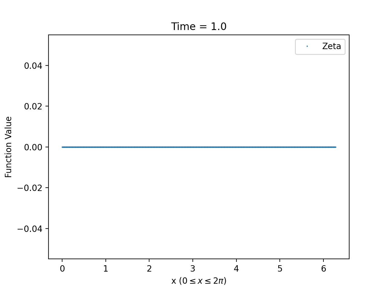
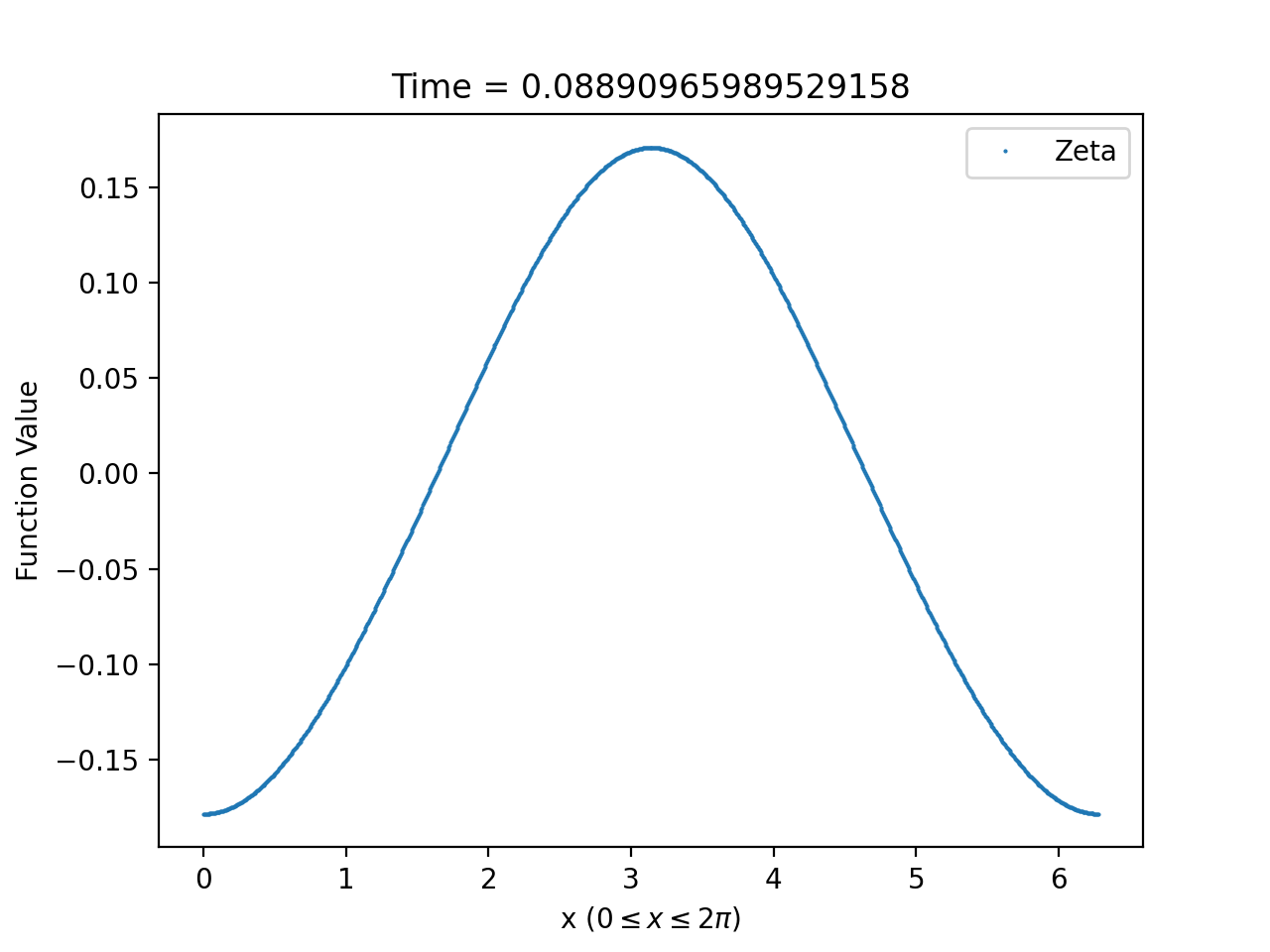
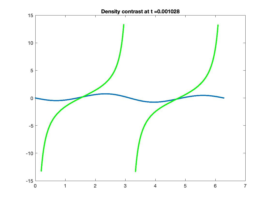
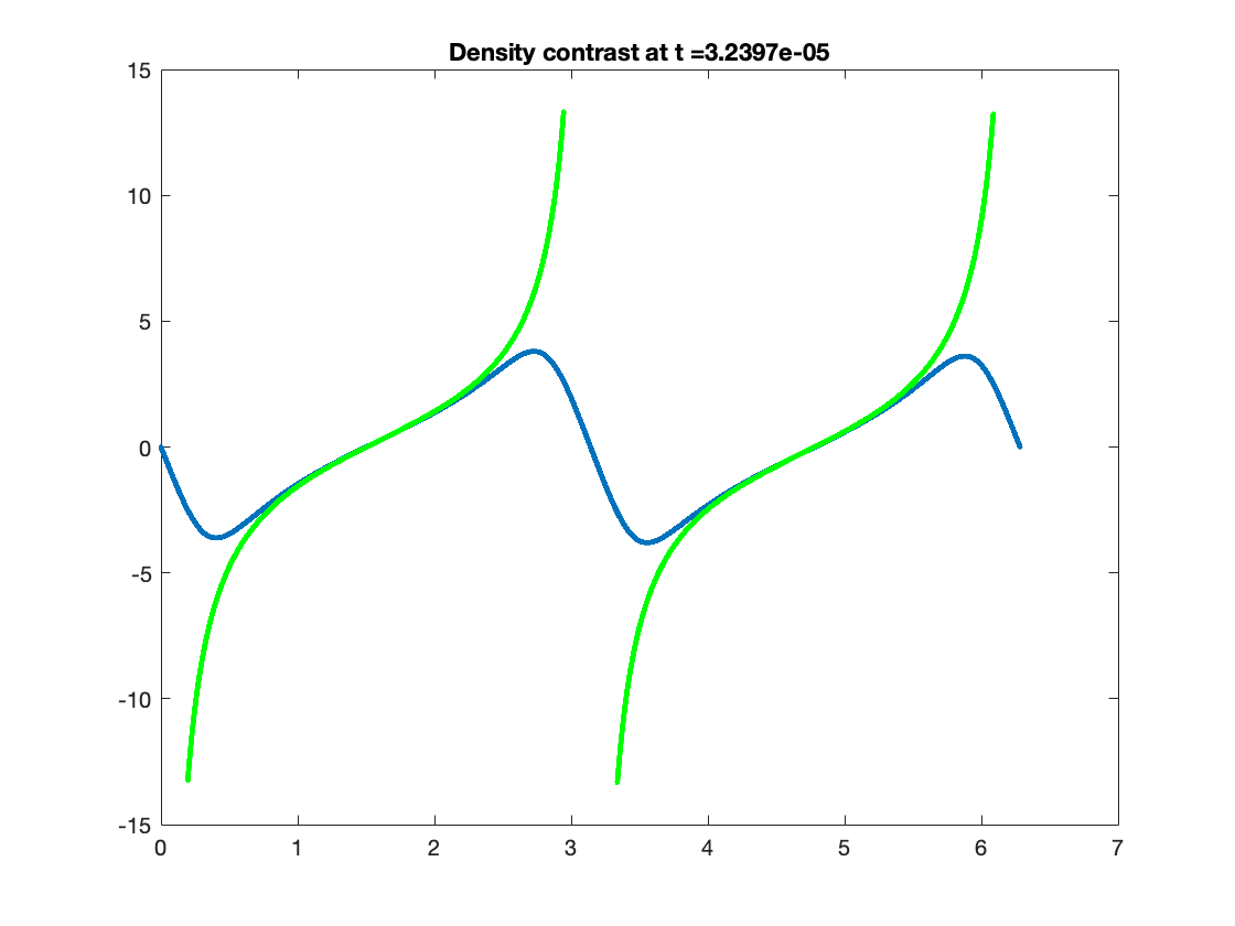
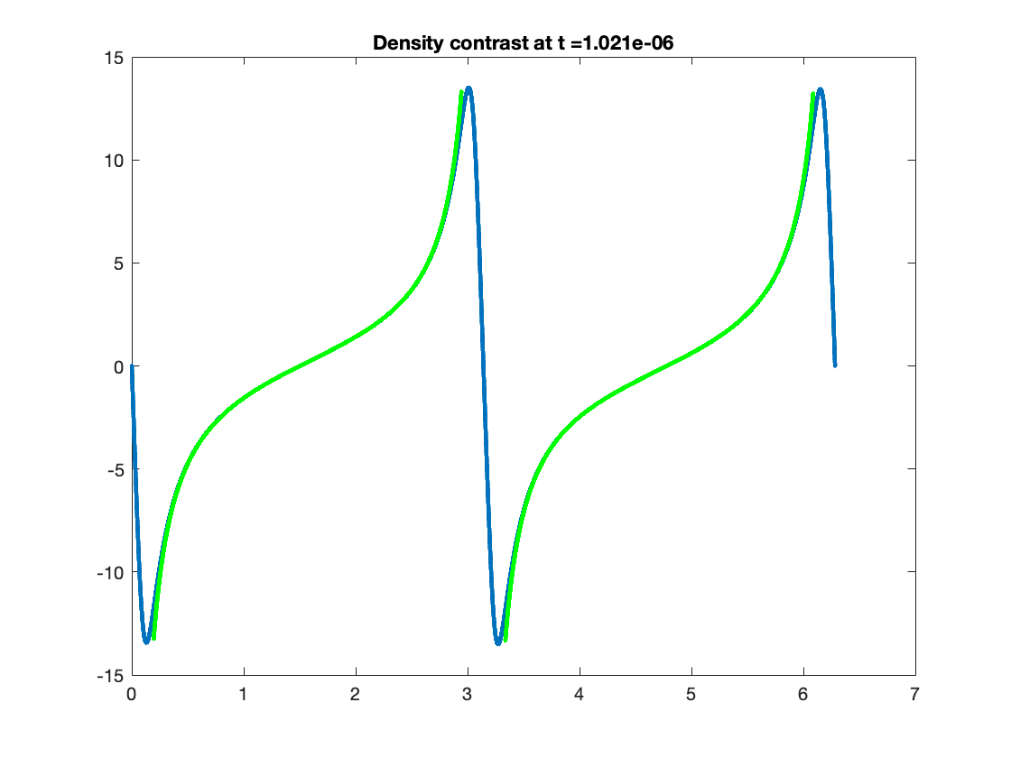
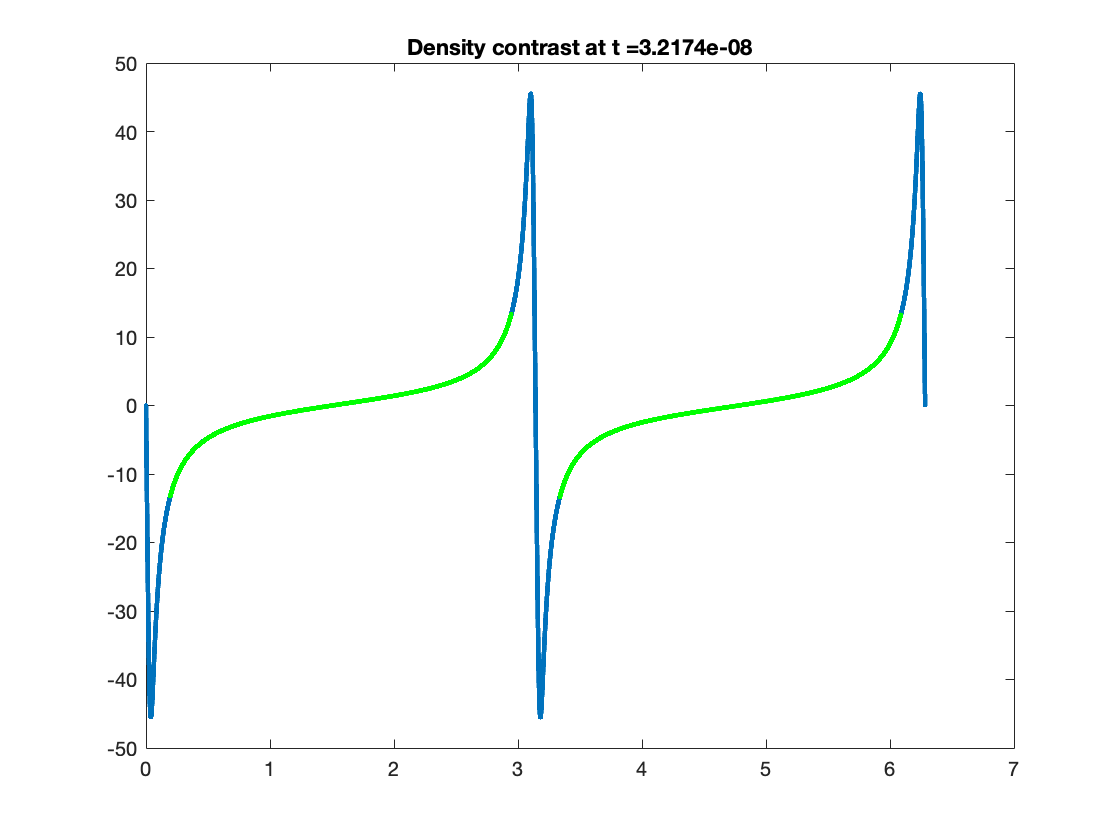
3.2.3. Behaviour of the density contrast
By (1.14), (1.17), (1.25) and (1.56)-(1.57), the density can be written in terms of z and w as where . Differentiating this expression, we find after a short calculation that the density contrast is given by
| (3.12) |
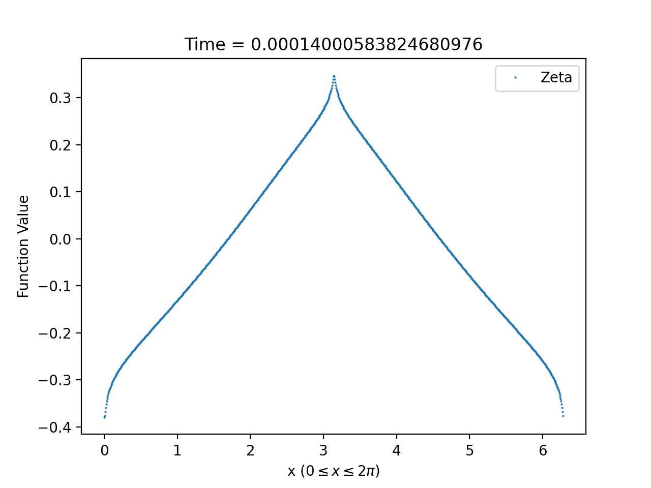
Using this formula to compute the density contrast for numerical solutions of (1.58)-(1.59), we observe from our numerical solutions that density contrast displays markedly different behaviour depending on whether or not it is generated from initial data satisfying (3.2). For solutions generated from initial data satisfying (3.2), we find that the density contrast remains bounded and converges as to a fixed function, which is expected by Theorem 1.2. An example of this behaviour is provided in Figure 9. On the other hand, the density contrast of solutions generated from initial data violating (3.2) develop steep gradients and blows-up at at isolated spatial points; see Figure 10 for an example of this behaviour.
As in Section 3.2.2, we can compare the density contrast of the full numerical solutions with the density contrast computed from a solutions of the asymptotic equation. We do this by evaluating (3.12) at and using (3.11) to approximate the density contrast at by
This formula identifies, at least heuristically, that the blow-up at in the density density contrast is due the vanishing of . Once again the agreement between the numerical and asymptotic plots is close enough that the two are practically indistinguishable as can be seen from Figure 11.
Acknowledgements
We thank Florian Beyer for helpful discussions and suggestions regarding the numerical aspects of this article.
References
- [1] F. Beyer and T.A. Oliynyk, Relativistic perfect fluids near Kasner singularities, preprint [arXiv:2012.03435], 2020.
- [2] F. Beyer, T.A. Oliynyk, and J.A Olvera-SantaMaría, The Fuchsian approach to global existence for hyperbolic equations, Comm. Part. Diff. Eqn. 46 (2021), 864–934.
- [3] D. Christodoulou, The formation of shocks in 3-dimensional fluids, EMS, 2007.
- [4] D. Fajman, T.A. Oliynyk, and Zoe Wyatt, Stabilizing relativistic fluids on spacetimes with non-accelerated expansion, Commun. Math. Phys. 383 (2021), 401–426.
- [5] G. Fournodavlos, Future dynamics of FLRW for the massless-scalar field system with positive cosmological constant, J. Math. Phys. 63 (2022), 032502.
- [6] H. Friedrich, Sharp asymptotics for Einstein--dust flows, Comm. Math. Phys. 350 (2017), 803 – 844.
- [7] R. Geroch, Faster than light?, preprint [arXiv:1005.1614 ], 2010.
- [8] M. Hadžić and J. Speck, The global future stability of the FLRW solutions to the Dust-Einstein system with a positive cosmological constant, J. Hyper. Differential Equations 12 (2015), 87–188.
- [9] P.G. LeFloch and Changhua Wei, The nonlinear stability of self-gravitating irrotational Chaplygin fluids in a FLRW geometry, Annales de l’Institut Henri Poincaré C, Analyse non linéaire 38 (2021), 757–814.
- [10] C. Liu and T.A. Oliynyk, Cosmological Newtonian limits on large spacetime scales, Commun. Math. Phys. 364 (2018), 1195–1304.
- [11] by same author, Newtonian limits of isolated cosmological systems on long time scales, Annales Henri Poincaré 19 (2018), 2157–2243.
- [12] C. Liu and C. Wei, Future stability of the FLRW spacetime for a large class of perfect fluids, Ann. Henri Poincaré 22 (2021), 715–779.
- [13] C. Lübbe and J. A. Valiente Kroon, A conformal approach for the analysis of the non-linear stability of radiation cosmologies, Annals of Physics 328 (2013), 1–25.
- [14] T. A. Oliynyk, Future stability of the FLRW fluid solutions in the presence of a positive cosmological constant, Commun. Math. Phys. 346 (2016), 293–312; see the preprint [arXiv:1505.00857] for a corrected version.
- [15] T.A. Oliynyk, The cosmological Newtonian limit on cosmological scales, Commun. Math. Phys. 339 (2015), 455–512.
- [16] by same author, Future global stability for relativistic perfect fluids with linear equations of state where , SIAM J. Math. Anal. 53 (2021), 4118–4141.
- [17] J. Rauch, Hyperbolic partial differential equations and geometric optics, AMS, 2012.
- [18] A. D. Rendall, Asymptotics of solutions of the Einstein equations with positive cosmological constant, Ann. Henri Poincaré 5 (2004), no. 6, 1041–1064.
- [19] H. Ringstöm, Future stability of the Einstein-non-linear scalar field system, Invent. Math. 173 (2008), 123–208.
- [20] I. Rodnianski and J. Speck, The stability of the irrotational Euler-Einstein system with a positive cosmological constant, J. Eur. Math. Soc. 15 (2013), 2369–2462.
- [21] K. Schneider, D. Kolomenskiy, and E. Deriaz, Is the CFL condition sufficient? Some remarks, The Courant-Friedrichs-Lewy (CFL) Condition - 80 Years after its discovery (Unknown, Unknown Region) (C. A. De Moura and C. S. Kubrusly, eds.), 2013, pp. 139–146.
- [22] J. Speck, The nonlinear future-stability of the FLRW family of solutions to the Euler-Einstein system with a positive cosmological constant, Selecta Mathematica 18 (2012), 633–715.
- [23] by same author, The stabilizing effect of spacetime expansion on relativistic fluids with sharp results for the radiation equation of state, Arch. Rat. Mech. 210 (2013), 535–579.
- [24] M.E. Taylor, Partial differential equations III: Nonlinear equations, Springer, 1996.
- [25] A.D. Rendall U. Brauer and O. Reula, The cosmic no-hair theorem and the non-linear stability of homogeneous Newtonian cosmological models, Class. Quant. Grav 11 (1994), 2283–2296.
- [26] C. Wei, Stabilizing effect of the power law inflation on isentropic relativistic fluids, Journal of Differential Equations 265 (2018), 3441 – 3463.