11email: {babak,samal}@iuuk.mff.cuni.cz
On the time complexity of finding a well-spread perfect matching in bridgeless cubic graphs††thanks: Supported by the project GAUK182623 of the Charles University Grant Agency and by grant 25-16627SS of the Czech Science Foundation.
Abstract
We present an algorithm for finding a perfect matching in a -edge-connected cubic graph that intersects every -edge cut in exactly one edge. Specifically, we propose an algorithm with a time complexity of , which significantly improves upon the previously known -time algorithms for the same problem. The technique we use for the improvement is efficient use of cactus model of 3-edge cuts. As an application, we use our algorithm to compute embeddings of -edge-connected cubic graphs with limited number of singular edges (i.e., edges that are twice in the boundary of one face) in time; this application contributes to the study of the well-known Cycle Double Cover conjecture.
Keywords:
Algorithm Perfect matching Cut representation Embedding1 Introduction
It is well known that every bridgeless cubic graph admits a perfect matching [Pet91]. Using Edmonds’ blossom algorithm, a maximum matching can be found in polynomial time. Gabow [Gab90] demonstrated that the weighted matching problem on general graphs can be solved in time .
Consequently, the minimum weight perfect matching problem for bridgeless cubic graphs can be solved in time. Diks and Stańczyk [DS10] proposed an improved algorithm for finding perfect matchings in bridgeless cubic graphs with time complexity of .
In this paper we study the complexity of finding a perfect matching in a bridgeless cubic graph such that in every 3-edge cut contains exactly one edge. By parity, can contain one or three edges in a 3-edge cut; so our condition says no 3-edge cut is contained in . We shortly express this by saying is well spread.
Kaiser et al. [KKN06] showed that a wells spread perfect matching exists in every bridgeless cubic graph (and went on to use this to find how much of the graph can be covered by two, three, etc. perfect matchings). Their proof uses Edmonds perfect matching polytope (vector is a fractional perfect matching, thus it is a convex combination of perfect matchings – each of them is well spread). This, however, doesn’t yield an efficient algorithm.
In [BIT13], Boyd et al. focus on developing algorithms for finding -factors in bridgeless cubic graphs that cover specific edge-cuts, which brings these -factors closer to Hamiltonian cycles. They provide an efficient algorithm that finds a minimum-weight -factor that covers all -edge cuts in weighted bridgeless cubic graphs (in contrast with finding a Hamiltonian cycle, which is computationally hard). They also provide both a polyhedral description of such -factors and of their complements – well spread perfect matchings. This is the first known polynomial-time algorithm for this problem, with a time complexity of , where is the number of vertices. In this work, we improve this result for -edge-connected cubic graphs using Algorithm 1 with time complexity .
Boyd et al. find a “peripheral 3-edge-cut” (a cut such that one side of it is internally 4-edge-connected) and then use recursion. We save computation by using the cactus model, also called a tree of cuts. In this tree it is easy to find the peripheral cut and also to update the tree when we contract a part of the cut. This leads to much improved time complexity, although only for 3-edge-connected graphs.
We then proceed to apply this result to the study of the well-known Cycle Double Cover (or CDC) Conjecture [Sze73, Sey79]. In the language of graph embedding, CDC conjecture is equivalent to every bridgeless cubic graph having a surface embedding with no singular edges (i.e., with no edge that is on the boundary of one face twice). As an application of our work, for a -edge-connected cubic graph we can find embeddings with a bounded number of singular edges in time .
The structure of the paper is as follows. In the next section, we introduce the necessary definitions and concepts. In Section 3, we discuss the cactus model, a key component in deriving our results. Section 4 presents our main result, an efficient algorithm to find the well-spread perfect matching. Finally, in Section 5, we apply our algorithm to get results about the well-known CDC conjecture.
2 Preliminaries
Let be a graph with vertex set and edge set . A graph in which all vertices have degree is called cubic. A cycle is a connected -regular graph. A bridge in a graph is an edge whose removal increases the number of components of . Equivalently, a bridge is an edge that is not contained in any cycles of . A graph is bridgeless if it contains no bridge. An edge cut in a graph is a set of edges whose removal increases the number of connected components of the graph. An edge cut in is called a non-trivial cut if every component of has at least two vertices. Otherwise it is called trivial. A -edge-cut in a graph is an edge cut that contains exactly edges. A connected graph is -edge-connected if it remains connected whenever fewer than edges are removed. A graph is cyclically -edge-connected, if at least edges must be removed to disconnect it into two components such that each component contains a cycle. We say that a subset covers an edge-cut if . For a subset , is the graph obtained from by contracting all the edges in . Note that we keep multiple edges and only remove loops in such contraction.
Petersen’s theorem [Pet91] states that every bridgeless cubic graph contains a perfect matching. Schönberger [Sch35] proved the following strengthened form of Petersen’s theorem.
Theorem 2.1 ([Sch35])
Let be a bridgeless cubic graph with specified edge . Then there exists a perfect matching of G that contains .
A perfect matching containing a specified edge in a bridgeless cubic graph can be found in time [BBDL01].
A graph is embedded in a surface if the vertices of are distinct elements of and every edge of is a simple arc connecting in the two vertices which it joins in , such that its interior is disjoint from other edges and vertices. An embedding of a graph in is an isomorphism of with a graph embedded in .
Let be a graph that is cellularly embedded in a surface , that is, every face is homeomorphic to an open disk. Let where is the cyclic permutation of the edges incident with the vertex such that is the successor of in the clockwise ordering around . The cyclic permutation is called the local rotation at , and the set is the rotation system of the given embedding of in .
Let be a connected multigraph. A combinatorial embedding of is a pair where is a rotation system, and is a signature mapping which assigns to each edge a sign . If is an edge incident with , then the cyclic sequence is called the -clockwise ordering around (or the local rotation at ). Given an embedding of we say that is -embedded. It is known that the combinatorial embedding uniquely determines a cellular embedding to some surface, up to homeomorphism [MT01, Theorems 3.2.4 and 3.3.1].
A closed walk is a sequence where and for every , . We say that a collection of closed walks forms a partial circuit double cover (or partial CDC) if each edge is covered at most once by one of ’s or exactly twice by two different and , and for every vertex and edges and where , there exists at most one closed walk such that .
3 The cactus model
Here we follow the notations and definition of [NI08]. A general way to represent a subset of cuts within a graph involves constructing a cactus representation . In this representation, is a graph, and is a function mapping vertices from to . The cactus representation (or the cactus model) was introduced in [DKL76]. It was further utilized in [Gab91, Din93]. This model plays a crucial role in understanding both edge connectivity and graph rigidity problems.
Definition 1
Let be a graph. A pair with is called a cactus representation (or cactus model) for graph if it meets the following criteria:
-
1.
For an arbitrary minimum cut , the cut in defined by , and is a minimum cut in .
-
2.
Conversely, for every minimum cut in , there exists a minimum cut such that , and
In this context, we use vertex when referring to elements of and node for elements of . The set may include a node that does not correspond to any vertex with ; such a node is referred to as an empty node. We use for the set of all minimum cuts in .
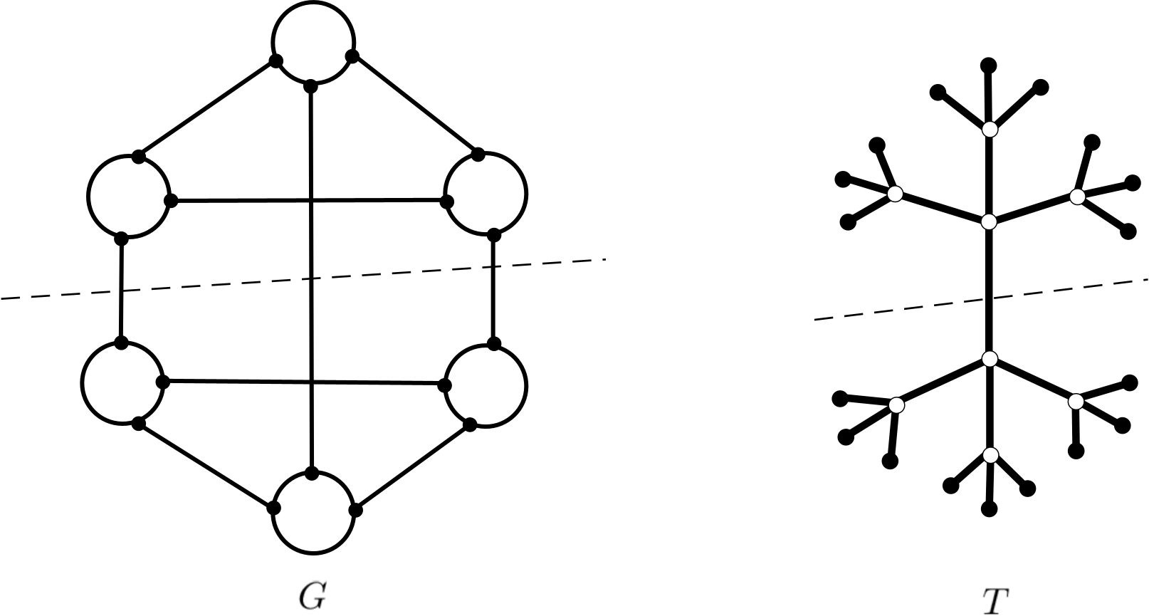
It was shown in [DKL76] that every has a cactus representation using a cactus graph – a multigraph where every edge is exactly one cycle. A special case of such graph is a tree with every edge doubled. It is known that when the connectivity is odd, the cactus representation is of this special type. In this case we will just call it a tree of cuts (or cactus tree). For a -edge-connected cubic graph , the vertices of the graph correspond to the leaf nodes of the cactus tree and all the interior nodes of are empty nodes (see Fig. 1). We will also use the following estimate for the size of .
Lemma 1 ([Din93])
Let be a -edge-connected cubic graph with vertices and let be its cactus tree. Then
4 Well spread perfect matchings in bridgeless cubic graphs
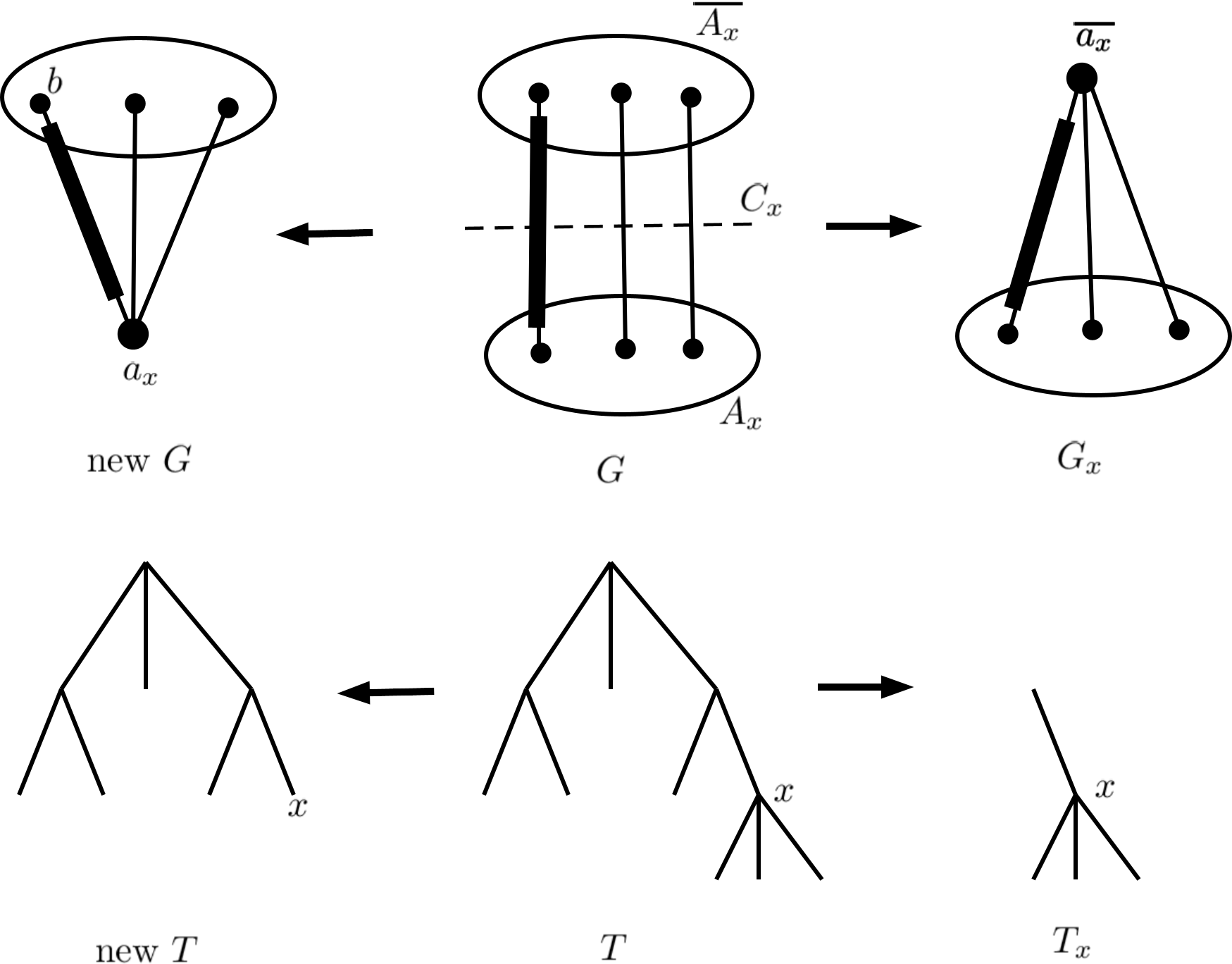
In this section, we present an algorithm that finds a perfect matching in a -edge-connected cubic graph that intersects all -edge cuts in exactly one edge and is substantially faster than the algorithm introduced by Boyd et al. [BIT13]. We first explain the underlying technique. Let be a graph with a 3-edge cut ; that is . We let (all vertices in are contracted to a single vertex ) and (with a new vertex ). A well-spread matching in contains exactly one edge of , thus it gives us a perfect matching in and in . As edges out of in and out of in are in natural correspondence with edges of , we will identify them and say that and agree on . For our algorithm the following is crucial.
Theorem 4.1
Let , , and be as above. Given a well-spread perfect matching in and in that agree on the cut , the union is a well-spread perfect matching in .
Proof
The fact that is a perfect matching is clear as these matchings agree on . The fact that is well-spread follows from the fact that 3-edge cuts in a 3-edge-connected graph do not cross, see [BIT13] for details. ∎
Boyd et al. [BIT13] use the above theorem together with repeated finding of a “peripheral 3-edge-cut” : one where is internally 4-edge-connected. We refine their approach by utilizing (and updating) the model for all 3-edge cuts that will allow us to find peripheral cuts quickly. Also, we will use the model of the cuts to quickly decompose the graph in and and then combine them back.
We will also use the following information about structure of cuts in and .
Theorem 4.2
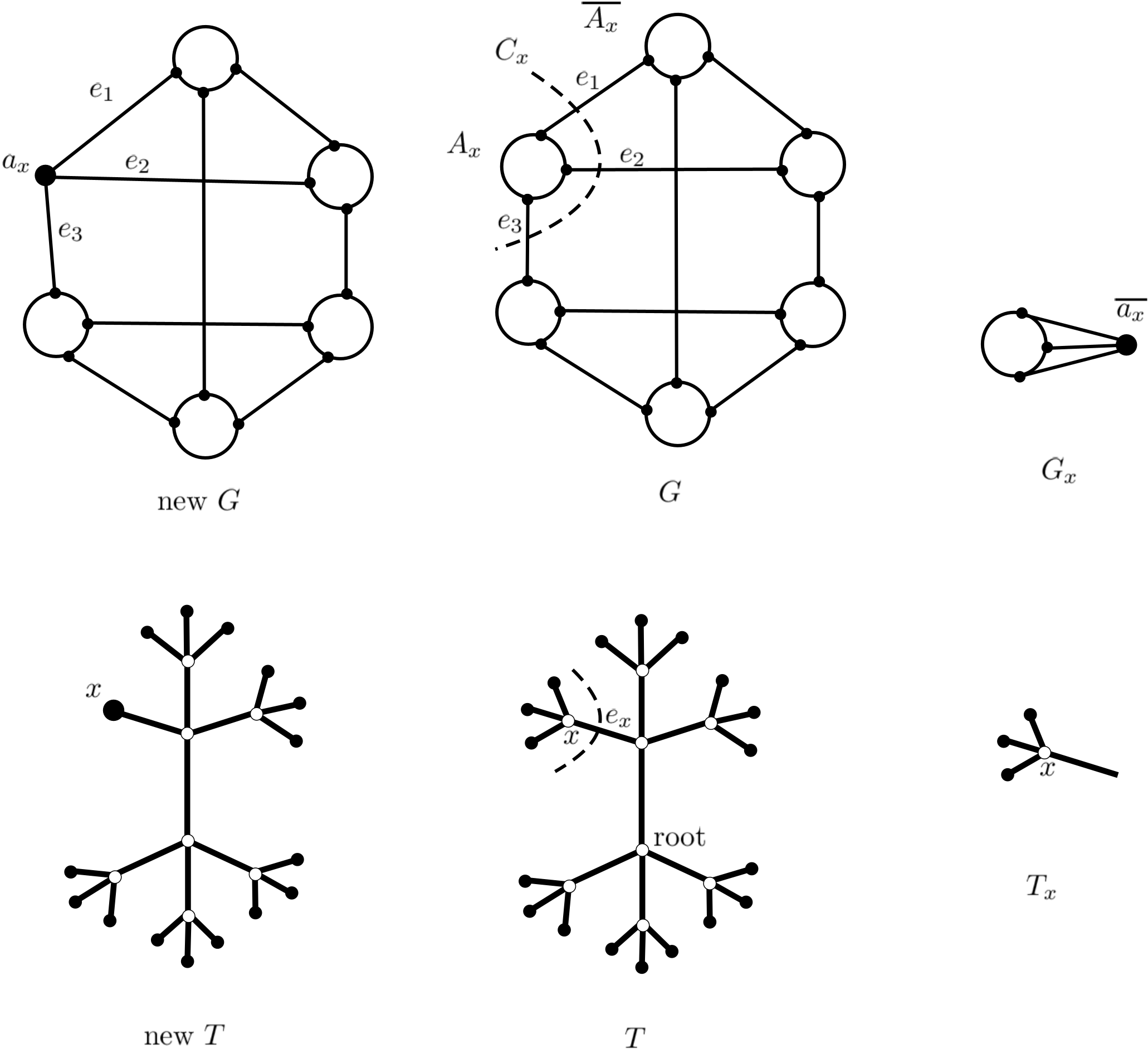
Let , , and be as above. Let be the cactus tree for . Let be the edge of corresponding to ; that is the components of are , , and . Put for . Define as a restriction of to and put . We define symmetrically.
Then is the cactus tree representation of 3-edge cuts in (for ).
The proof follows the same idea as that of Theorem 4.1: minimum odd edge-cuts do not cross. We omit the details in this extended abstract.
In our application we have a 3-regular 3-edge-connected graph, so all vertices are mapped to leaf nodes of the cactus tree and nontrivial 3-cuts correspond to edges that are not incident with a leaf. In particular, when the cactus tree is a star there are no nontrivial 3-cuts and we may simply find any perfect matching. In a sense, the purpose of our algorithm is to efficiently combine matchings coming from these “special cases” of internally 4-edge-connected graphs.
To this end, we pick root in the cut model . Let be the edge connecting to its parent. We let be the three edges in the cut corresponding to . We let be the vertices of that are mapped by to descendants of (including ), so that .
We do not use this definition directly, instead we recursively update , while traversing the tree. We can compute as a union of for all children of . We can compute by going over for all children of , excluding edges that lead withing (between and for two children of ). To do this efficiently we utilize the Union-Find algorithm.
In a typical step of decomposition part of the algorithm, we use Theorem 4.2, with the new graphs being (which we store for later) and updated version of . To illustrate the algorithm, in Figure 2 we show one step including the updated trees. We see that is a star – which means is internally 4-edge-connected. Updated simply removes children of . However, we actually do not need to update and compute in the algorithm.
In a typical step of assembling part of the algorithm, we use Theorem 4.1. For graph we have our well-spread matching from the recursion. For the other graph, , we compute it easily, as the graph is internally 4-edge-connected, so any perfect matching will do. Figure 3 illustrates this part of the algorithm.
Theorem 4.3
The output of Algorithm 1 is a well spread perfect matching.
4.1 Complexity Analysis
The construction of the tree of cuts (the cactus model) can be done in time [Gab91]. By Lemma 1 we have . Next, the algorithm decomposes the graph along -edge cuts. Here the main work is keeping track of the sets and , updating the graph and . For this we use the standard Union-Find algorithm plus a constant amount of work for changing three edges of the cut at each step. Thus the total time required for this loop is .
In the assembly step, we repeatedly look for a perfect matching in an internally 4-edge-connected cubic graph containing a given edge. By [BBDL01], this can be done in time . (The initial step where is the root is faster, as we don’t need to specify an edge, but this bound works as well.) The remaining work (combining the matchings) needs only a constant time per edge, so linear in total.
Note that is the degree of in ; let denote this quantity. We know that . The time complexity is thus
So the leading term in the time complexity is the final sum. As the function is convex, the sum will be maximal when one is as large as possible (namely, ) and the other as small as possible (namely, 1) – otherwise we can increase the sum of , while keeping sum of constant. For this extreme case we get our bound for time complexity of the algorithm, .
Theorem 4.4
Algorithm 1 finds a well spread perfect matching in a -edge-connected cubic graph in time .
5 Application
In [GŠ24], Ghanbari and Šamal establish an upper bound of on the number of singular edges in an embedding of a bridgeless cubic graph on a surface. They also raise the question of how efficiently one can find a perfect matching in a bridgeless cubic graph that contains no odd cut of size — an essential step in determining the time complexity of finding such an embedding. Here, we answer their question for -edge connected cubic graphs and describe an algorithm that constructs an embedding with at most bad edges. To provide context, we first state their results.
Lemma 2 ([GŠ24])
Let be a bridgeless cubic graph, and be a collection of closed walks in . If form a partial CDC, then there is an embedding of where are some of the facial walks of . Moreover, such an embedding can be found by a linear time algorithm.
Theorem 5.1 ([GŠ24])
Let be a bridgeless cubic graph. There exists an embedding of with at most singular edges.
To prove Theorem 5.1, in [GŠ24], we first construct a perfect matching such that contains no odd cut of size 3. This guarantees the existence of another perfect matching satisfying (see [KKN06]). Next, we show that can be extended to an embedding using Lemma 2, where the potential singular edges of the embedding are precisely those in , and this completes their proof.
Suppose that the cubic graph is -edge-connected. To find , we employ Algorithm 1, which finds a perfect matching in time . Consequently, determining the overall time complexity reduces to finding the perfect matching . We utilize Diks and Stańczyk’s algorithm [DS10] to find in time . Thus, the embedding guaranteed by Theorem 5.1 can be found in total time
6 Conclusion
We studied a new approach to finding a perfect matching that includes all -edge cuts in a -edge-connected cubic graph, utilizing the cactus representation of the graph. We referred to such a perfect matching as well spread. In Section 4, we presented an algorithm that finds a well-spread perfect matching in a -edge-connected cubic graph in time .
In general, the best-known algorithm for finding a well-spread perfect matching in a bridgeless cubic graph has a time complexity of [BIT13]. In the future, it would be interesting to determine whether the cactus representation can be leveraged to develop a faster algorithm for finding such a well-spread perfect matching. However, the issue is that representing 3-edge-cuts in a graph that may contain 2-edge-cuts is more complicated.
References
- [BBDL01] Therese C. Biedl, Prosenjit Bose, Erik D. Demaine, and Anna Lubiw. Efficient algorithms for Petersen’s matching theorem. J. Algorithms, 38(1):110–134, 2001.
- [BIT13] Sylvia Boyd, Satoru Iwata, and Kenjiro Takazawa. Finding 2-factors closer to TSP tours in cubic graphs. SIAM Journal on Discrete Mathematics, 27(2):918–939, 2013.
- [Din93] Efim Dinitz. The 3-edge-components and a structural description of all 3-edge-cuts in a graph. In Ernst W. Mayr, editor, Graph-Theoretic Concepts in Computer Science, pages 145–157, Berlin, Heidelberg, 1993. Springer Berlin Heidelberg.
- [DKL76] E. Dinic, Alexander Karzanov, and M. Lomonosov. The system of minimum edge cuts in a graph. In book: Issledovaniya po Diskretnoǐ Optimizatsii (Engl. title: Studies in Discrete Optimizations), A.A. Fridman, ed., Nauka, Moscow, 290-306, in Russian,, 01 1976.
- [DS10] Krzysztof Diks and Piotr Stanczyk. Perfect matching for biconnected cubic graphs in time. In Jan van Leeuwen, Anca Muscholl, David Peleg, Jaroslav Pokorný, and Bernhard Rumpe, editors, SOFSEM 2010: Theory and Practice of Computer Science, pages 321–333, Berlin, Heidelberg, 2010. Springer Berlin Heidelberg.
- [Gab90] Harold N. Gabow. Data structures for weighted matching and nearest common ancestors with linking. In Proceedings of the First Annual ACM-SIAM Symposium on Discrete Algorithms, SODA ’90, page 434–443, USA, 1990. Society for Industrial and Applied Mathematics.
- [Gab91] Harold N. Gabow. Applications of a poset representation to edge connectivity and graph rigidity. [1991] Proceedings 32nd Annual Symposium of Foundations of Computer Science, pages 812–821, 1991.
- [GŠ24] Babak Ghanbari and Robert Šámal. Approximate cycle double cover. In Adele Anna Rescigno and Ugo Vaccaro, editors, Combinatorial Algorithms, pages 421–432, Cham, 2024. Springer Nature Switzerland.
- [KKN06] Tomáš Kaiser, Daniel Král’, and Serguei Norine. Unions of perfect matchings in cubic graphs. In Martin Klazar, Jan Kratochvíl, Martin Loebl, Jiří Matoušek, Pavel Valtr, and Robin Thomas, editors, Topics in Discrete Mathematics, pages 225–230, Berlin, Heidelberg, 2006. Springer Berlin Heidelberg.
- [MT01] Bojan Mohar and Carsten Thomassen. Graphs on Surfaces. Johns Hopkins series in the mathematical sciences. Johns Hopkins University Press, 2001.
- [NI08] Hiroshi Nagamochi and Toshihide Ibaraki. Algorithmic aspects of graph connectivity. Encyclopedia of mathematics and its applications ; v. 123. Cambridge University Press, Cambridge, 2008.
- [Pet91] Julius Petersen. Die Theorie der regulären graphs. Acta Math., 15(1):193–220, 1891.
- [Sch35] Tibor Schönberger. Ein beweis des petersenschen graphensatzes. Acta litterarum ac scientiarum Regiae Universitatis Hungaricae Francisco-Josephinae: Sectio scientiarum mathematicarum, 7:51–57, 1935.
- [Sey79] Paul D Seymour. Sums of circuits. Graph theory and related topics, 1:341–355, 1979.
- [Sze73] G. Szekeres. Polyhedral decompositions of cubic graphs. Bulletin of the Australian Mathematical Society, 8(3):367–387, 1973.