This paper was converted on www.awesomepapers.org from LaTeX by an anonymous user.
Want to know more? Visit the Converter page.

On the use of approximate Bayesian computation Markov chain Monte Carlo with inflated tolerance and post-correction

Matti Vihola  and  Jordan Franks Department of Mathematics and Statistics, University of Jyväskylä P.O.Box 35, FI-40014 University of Jyväskylä, Finland matti.s.vihola@jyu.fi, jordan.j.franks@jyu.fi
Abstract.

Approximate Bayesian computation allows for inference of complicated probabilistic models with intractable likelihoods using model simulations. The Markov chain Monte Carlo implementation of approximate Bayesian computation is often sensitive to the tolerance parameter: low tolerance leads to poor mixing and large tolerance entails excess bias. We consider an approach using a relatively large tolerance for the Markov chain Monte Carlo sampler to ensure its sufficient mixing, and post-processing the output leading to estimators for a range of finer tolerances. We introduce an approximate confidence interval for the related post-corrected estimators, and propose an adaptive approximate Bayesian computation Markov chain Monte Carlo, which finds a ‘balanced’ tolerance level automatically, based on acceptance rate optimisation. Our experiments show that post-processing based estimators can perform better than direct Markov chain targetting a fine tolerance, that our confidence intervals are reliable, and that our adaptive algorithm leads to reliable inference with little user specification.

Key words and phrases:
Adaptive, approximate Bayesian computation, confidence interval, importance sampling, Markov chain Monte Carlo, tolerance choice

1. Introduction

Approximate Bayesian computation is a form of likelihood-free inference (see, e.g., the reviews Marin et al., 2012; Sunnåker et al., 2013) which is used when exact Bayesian inference of a parameter θ𝖳\theta\in\mathsf{T} with posterior density π(θ)pr(θ)L(θ)\pi(\theta)\propto\mathrm{pr}(\theta)L(\theta) is impossible, where pr(θ)\mathrm{pr}(\theta) is the prior density and L(θ)=g(yθ)L(\theta)=g(y^{*}\mid\theta) is an intractable likelihood with data y𝖸y^{*}\in\mathsf{Y}. More specifically, when the generative model of observations g(θ)g(\,\cdot\,\mid\theta) cannot be evaluated, but allows for simulations, we may perform relatively straightforward approximate inference based on the following (pseudo-)posterior:

(1) πϵ(θ)pr(θ)Lϵ(θ),whereLϵ(θ)=𝔼[Kϵ(Yθ,y)],Yθg(θ),\pi_{\epsilon}(\theta)\propto\mathrm{pr}(\theta)L_{\epsilon}(\theta),\qquad\text{where}\qquad L_{\epsilon}(\theta)=\mathbb{E}[K_{\epsilon}(Y_{\theta},y^{*})],\quad Y_{\theta}\sim g(\,\cdot\,\mid\theta),

where ϵ>0\epsilon>0 is a ‘tolerance’ parameter, and Kϵ:𝖸2[0,)K_{\epsilon}:\mathsf{Y}^{2}\to[0,\infty) is a ‘kernel’ function, which is often taken as a simple cut-off Kϵ(y,y)=1(s(y)s(y)ϵ)K_{\epsilon}(y,y^{*})=1\left(\|s(y)-s(y^{*})\|\leq\epsilon\right), where s:𝖸ds:\mathsf{Y}\to\mathbb{R}^{d} extracts a vector of summary statistics from the (pseudo) observations.

The summary statistics are often chosen based on the application at hand, and reflect what is relevant for the inference task; see also (Fearnhead and Prangle, 2012; Raynal et al., to appear). Because Lϵ(θ)L_{\epsilon}(\theta) may be regarded as a smoothed version of the true likelihood g(yθ)g(y^{*}\mid\theta) using the kernel KϵK_{\epsilon}, it is intuitive that using a too large ϵ\epsilon may blur the likelihood and bias the inference. Therefore, it is generally desirable to use as small a tolerance ϵ>0\epsilon>0 as possible, but because the computational methods suffer from inefficiency with small ϵ\epsilon, the choice of tolerance level is difficult (cf. Bortot et al., 2007; Sisson and Fan, 2018; Tanaka et al., 2006).

We discuss simple post-processing procedure which allows for consideration of a range of values for the tolerance ϵδ\epsilon\leq\delta, based on a single run of approximate Bayesian computation Markov chain Monte Carlo (Marjoram et al., 2003) with tolerance δ\delta. Such post-processing was suggested in (Wegmann et al., 2009) (in case of simple cut-off), and similar post-processing has been suggested also with regression adjustment (Beaumont et al., 2002) (in a rejection sampling context). The method, discussed further in Section 2, can be useful for two reasons: A range of tolerances ϵδ\epsilon\leq\delta may be routinely inspected, which can reveal excess bias in the pseudo-posterior πδ\pi_{\delta}; and the Markov chain Monte Carlo inference may be implemented with sufficiently large δ\delta to allow for good mixing.

Our contribution is two-fold. We suggest straightforward-to-calculate approximate confidence intervals for the posterior mean estimates calculated from the post-processing output, and discuss some theoretical properties related to it. We also introduce an adaptive approximate Bayesian computation Markov chain Monte Carlo which finds a balanced δ\delta during burn-in, using acceptance rate as a proxy, and detail a convergence result for it.

2. Post-processing over a range of tolerances

For the rest of the paper, we assume that the kernel function in (1) has the form

Kϵ(y,y)=ϕ(d(y,y)/ϵ),K_{\epsilon}(y,y^{*})=\phi\big{(}d(y,y^{*})/\epsilon\big{)},

where d:𝖸2[0,)d:\mathsf{Y}^{2}\to[0,\infty) is any ‘dissimilarity’ function and ϕ:[0,)[0,1]\phi:[0,\infty)\to[0,1] is a non-increasing ‘cut-off’ function. Typically d(y,y)=s(y)s(y)d(y,y^{*})=\|s(y)-s(y^{*})\|, where s:𝖸2ds:\mathsf{Y}^{2}\to\mathbb{R}^{d} are the chosen summaries, and in case of the simple cut-off discussed in Section 1, ϕ(t)=ϕsimple(t)=1(t1)\phi(t)=\phi_{\mathrm{simple}}(t)=1\left(t\leq 1\right). We will implicitly assume that the pseudo-posterior πϵ\pi_{\epsilon} given in (1) is well-defined for all ϵ>0\epsilon>0 of interest, that is, cϵ=pr(θ)Lϵ(θ)dθ>0c_{\epsilon}=\int\mathrm{pr}(\theta)L_{\epsilon}(\theta)\mathrm{d}\theta>0.

The following summarises the approximate Bayesian computation Markov chain Monte Carlo algorithm of Marjoram et al. (2003), with proposal qq and tolerance δ>0\delta>0:

Algorithm 1 (abc-mcmc(δ\delta)).

Suppose Θ0𝖳\Theta_{0}\in\mathsf{T} and Y0𝖸Y_{0}\in\mathsf{Y} are any starting values, such that pr(Θ0)>0\mathrm{pr}(\Theta_{0})>0 and ϕ(d(Y0,y)/δ)>0\phi(d(Y_{0},y^{*})/\delta)>0. For k=1,2,k=1,2,\ldots, iterate:

  1. (i)

    Draw Θ~kq(Θk1,)\tilde{\Theta}_{k}\sim q(\Theta_{k-1},\,\cdot\,) and Y~kg(Θ~k)\tilde{Y}_{k}\sim g(\,\cdot\,\mid\tilde{\Theta}_{k}).

  2. (ii)

    With probability αδ(Θk1,Yk1;Θ~k,Y~k)\alpha_{\delta}(\Theta_{k-1},Y_{k-1};\tilde{\Theta}_{k},\tilde{Y}_{k}) accept and set (Θk,Yk)(Θ~k,Y~k)(\Theta_{k},Y_{k})\leftarrow(\tilde{\Theta}_{k},\tilde{Y}_{k}); otherwise reject and set (Θk,Yk)(Θk1,Yk1)(\Theta_{k},Y_{k})\leftarrow(\Theta_{k-1},Y_{k-1}), where

    αδ(θ,y;θ~,y~)=min{1,pr(θ~)q(θ~,θ)ϕ(d(y~,y)/δ)pr(θ)q(θ,θ~)ϕ(d(y,y)/δ)}.\alpha_{\delta}(\theta,y;\tilde{\theta},\tilde{y})=\min\bigg{\{}1,\frac{\mathrm{pr}(\tilde{\theta})q(\tilde{\theta},\theta)\phi\big{(}d(\tilde{y},y^{*})/\delta\big{)}}{\mathrm{pr}(\theta)q(\theta,\tilde{\theta})\phi\big{(}d(y,y^{*})/\delta\big{)}}\bigg{\}}.

Algorithm 1 may be implemented by storing only Θk\Theta_{k} and the related distances Tk=d(Yk,y)T_{k}=d(Y_{k},y^{*}), and in what follows, we regard either (Θk,Yk)k1(\Theta_{k},Y_{k})_{k\geq 1} or (Θk,Tk)k1(\Theta_{k},T_{k})_{k\geq 1} as the output of Algorithm 1. In practice, the initial values (Θ0,Y0)(\Theta_{0},Y_{0}) should be taken as the state of the Algorithm 1 run for a number of initial ‘burn-in’ iterations. We also introduce an adaptive algorithm for parameter tuning later (Section 4).

It is possible to consider a variant of Algorithm 1 where many (possibly dependent) observations Y~k(1),,Y~k(m)g(Θ~k)\tilde{Y}_{k}^{(1)},\ldots,\tilde{Y}_{k}^{(m)}\sim g(\,\cdot\,\mid\tilde{\Theta}_{k}) are simulated in each iteration, and an average of their kernel values is used in the accept-reject step (cf. Andrieu et al., 2018). We focus here in the case of single pseudo-observation per iteration, following the asymptotic efficiency result of Bornn et al. (2017), but remark that our method may be applied in a straightforward manner also with multiple observations.

Definition 2.

Suppose (Θk,Tk)k=1,,n(\Theta_{k},T_{k})_{k=1,\ldots,n} is the output of abc-mcmc(δ\delta) for some δ>0\delta>0. For any ϵ(0,δ]\epsilon\in(0,\delta] such that ϕ(Tk/ϵ)>0\phi(T_{k}/\epsilon)>0 for some k=1,,nk=1,\ldots,n, and for any function f:𝖳f:\mathsf{T}\to\mathbb{R}, define

Uk(δ,ϵ)\displaystyle U_{k}^{(\delta,\epsilon)} =ϕ(Tk/ϵ)/ϕ(Tk/δ),\displaystyle=\phi(T_{k}/\epsilon)\big{/}\phi(T_{k}/\delta), Wk(δ,ϵ)\displaystyle\qquad W_{k}^{(\delta,\epsilon)} =Uk(δ,ϵ)/j=1nUj(δ,ϵ),\displaystyle=U_{k}^{(\delta,\epsilon)}\big{/}\textstyle\sum_{j=1}^{n}U_{j}^{(\delta,\epsilon)},
Eδ,ϵ(f)\displaystyle E_{\delta,\epsilon}(f) =k=1nWk(δ,ϵ)f(Θk),\displaystyle=\textstyle\sum_{k=1}^{n}W_{k}^{(\delta,\epsilon)}f(\Theta_{k}), Sδ,ϵ(f)\displaystyle S_{\delta,\epsilon}(f) =k=1n(Wk(δ,ϵ))2{f(Θk)Eδ,ϵ(f)}2.\displaystyle=\textstyle\sum_{k=1}^{n}(W_{k}^{(\delta,\epsilon)})^{2}\big{\{}f(\Theta_{k})-E_{\delta,\epsilon}(f)\big{\}}^{2}.

Algorithm 11 in Appendix details how Eδ,ϵ(f)E_{\delta,\epsilon}(f) and Sδ,ϵ(f)S_{\delta,\epsilon}(f) can be calculated in O(nlogn)O(n\log n) time simultaneously for all ϵδ\epsilon\leq\delta in case of simple cut-off. The estimator Eδ,ϵ(f)E_{\delta,\epsilon}(f) approximates 𝔼πϵ[f(Θ)]\mathbb{E}_{\pi_{\epsilon}}[f(\Theta)] and Sδ,ϵ(f)S_{\delta,\epsilon}(f) may be used to construct a confidence interval; see Algorithm 5 below. Theorem 4 details consistency of Eδ,ϵ(f)E_{\delta,\epsilon}(f), and relates Sδ,ϵ(f)S_{\delta,\epsilon}(f) to the limiting variance, in case the following (well-known) condition ensuring a central limit theorem holds:

Assumption 3 (Finite integrated autocorrelation).

Suppose that 𝔼πϵ[f2(Θ)]<\mathbb{E}_{\pi_{\epsilon}}[f^{2}(\Theta)]<\infty and k1ρk(δ,ϵ)\sum_{k\geq 1}\rho_{k}^{(\delta,\epsilon)} is finite, with ρk(δ,ϵ)=Corr(hδ,ϵ(Θ0(s),Y0(s)),hδ,ϵ(Θk(s),Yk(s)))\rho_{k}^{(\delta,\epsilon)}=\mathrm{Corr}\big{(}h_{\delta,\epsilon}(\Theta_{0}^{(s)},Y_{0}^{(s)}),h_{\delta,\epsilon}(\Theta_{k}^{(s)},Y_{k}^{(s)})\big{)}, where (Θk(s),Yk(s))k1(\Theta_{k}^{(s)},Y_{k}^{(s)})_{k\geq 1} is a stationary version of the abc-mcmc(δ\delta) chain, and

hδ,ϵ(θ,y)=wδ,ϵ(y)f(θ)wherewδ,ϵ(y)=ϕ(d(y,y)/ϵ)/ϕ(d(y,y)/δ).h_{\delta,\epsilon}(\theta,y)=w_{\delta,\epsilon}(y)f(\theta)\qquad\text{where}\qquad w_{\delta,\epsilon}(y)=\phi\big{(}d(y,y^{*})/\epsilon\big{)}/\phi\big{(}d(y,y^{*})/\delta\big{)}.
Theorem 4.

Suppose (Θk,Tk)k1(\Theta_{k},T_{k})_{k\geq 1} is the output of abc-mcmc(δ\delta), and denote by Eδ,ϵ(n)(f)E_{\delta,\epsilon}^{(n)}(f) and Sδ,ϵ(n)(f)S_{\delta,\epsilon}^{(n)}(f) the estimators in Definition 2. If (Θk,Tk)k1(\Theta_{k},T_{k})_{k\geq 1} is φ\varphi-irreducible (Meyn and Tweedie, 2009) then, for any ϵ(0,δ)\epsilon\in(0,\delta), we have as nn\to\infty:

  1. (i)

    Eδ,ϵ(n)(f)𝔼πϵ[f(Θ)]E_{\delta,\epsilon}^{(n)}(f)\to\mathbb{E}_{\pi_{\epsilon}}[f(\Theta)] almost surely, whenever the expectation is finite.

  2. (ii)

    Under Assumption 3, n1/2(Eδ,ϵ(n)(f)𝔼πϵ[f(Θ)])N(0,vδ,ϵ(f)τδ,ϵ(f))n^{1/2}\big{(}E_{\delta,\epsilon}^{(n)}(f)-\mathbb{E}_{\pi_{\epsilon}}[f(\Theta)]\big{)}\to N\big{(}0,v_{\delta,\epsilon}(f)\tau_{\delta,\epsilon}(f)\big{)} in distribution, where τδ,ϵ(f)=(1+2k1ρk(δ,ϵ))[0,)\tau_{\delta,\epsilon}(f)=\big{(}1+2\sum_{k\geq 1}\rho_{k}^{(\delta,\epsilon)}\big{)}\in[0,\infty) and nSδ,ϵ(n)(f)vδ,ϵ(f)[0,)nS_{\delta,\epsilon}^{(n)}(f)\to v_{\delta,\epsilon}(f)\in[0,\infty) almost surely.

Proof of Theorem 4 is given in Appendix. Inspired by Theorem 4, we suggest to report the following approximate confidence intervals for the suggested estimators:

Algorithm 5.

Suppose (Θk,Tk)k=1,,n(\Theta_{k},T_{k})_{k=1,\ldots,n} is the output of abc-mcmc(δ\delta) and f:Θf:\Theta\to\mathbb{R} is a function, then for any ϵδ\epsilon\leq\delta:

  1. (i)

    Calculate Eδ,ϵ(f)E_{\delta,\epsilon}(f) and Sδ,ϵ(f)S_{\delta,\epsilon}(f) as in Definition 2 (or in Algorithm 11).

  2. (ii)

    Calculate τ^δ(f)\hat{\tau}_{\delta}(f), an estimate of the integrated autocorrelation of (f(Θk))k=1,,n\big{(}f(\Theta_{k})\big{)}_{k=1,\ldots,n}.

  3. (iii)

    Report the confidence interval

    [Eδ,ϵ(f)±zq(Sδ,ϵ(f)τ^δ(f))1/2],\big{[}E_{\delta,\epsilon}(f)\pm z_{q}\big{(}S_{\delta,\epsilon}(f)\hat{\tau}_{\delta}(f)\big{)}^{1/2}\big{]},

    where zq>0z_{q}>0 corresponds to the desired normal quantile.

The confidence interval in Algorithm 5 is straightforward application of Theorem 4, except for using a common integrated autocorrelation estimate τ^δ(f)\hat{\tau}_{\delta}(f) for all τδ,ϵ(f)\tau_{\delta,\epsilon}(f). This relies on the approximation τδ,ϵ(f)τδ(f)\tau_{\delta,\epsilon}(f)\lessapprox\tau_{\delta}(f), which may not always be entirely accurate, but likely to be reasonable, as illustrated by Theorem 6 in Section 3 below. We suggest using a common τ^δ(f)\hat{\tau}_{\delta}(f) for all tolerances because direct estimation of integrated autocorrelation is computationally demanding, and likely to be unstable for small ϵ\epsilon.

The classical choice for τ^δ(f)\hat{\tau}_{\delta}(f) in Algorithm 5(ii) is windowed autocorrelation, τ^δ(f)=k=ω(k)ρ^k\hat{\tau}_{\delta}(f)=\sum_{k=-\infty}^{\infty}\omega(k)\hat{\rho}_{k}, with some 0ω(k)10\leq\omega(k)\leq 1, where ρ^k\hat{\rho}_{k} is the sample autocorrelation of (f(Θk))\big{(}f(\Theta_{k})\big{)} (cf. Geyer, 1992). We employ this approach in our experiments with ω(k)=1(|k|M)\omega(k)=1\left(|k|\leq M\right) where the cut-off lag MM is chosen adaptively as the smallest integer such that M5(1+2i=1Mρ^k)M\geq 5\big{(}1+2\sum_{i=1}^{M}\hat{\rho}_{k}\big{)} (Sokal, 1996). Also more sophisticated techniques for the calculation of the asymptotic variance have been suggested (e.g. Flegal and Jones, 2010).

We remark that, although we focus here on the case of using a common cut-off ϕ\phi for both the abc-mcmc(δ\delta) and the post-correction, one could also use a different cut-off ϕs\phi_{s} in the simulation phase, as considered by Beaumont et al. (2002) in the regression context. The extension to Definition 2 is straightforward, setting Uk(δ,ϵ)=ϕ(Tk/ϵ)/ϕs(Tk/δ)U_{k}^{(\delta,\epsilon)}=\phi(T_{k}/\epsilon)\big{/}\phi_{s}(T_{k}/\delta), and Theorem 4 remains valid under a support condition.

3. Theoretical justification

The following result, whose proof is given in Appendix, gives an expression for the integrated autocorrelation in case of simple cut-off.

Theorem 6.

Suppose Assumption 3 holds and ϕ=ϕsimple\phi=\phi_{\mathrm{simple}}, then

τδ,ϵ(f)1=(τˇδ,ϵ(f)1)varπδ(fδ,ϵ)+2πδ(θ)w¯δ,ϵ(θ)(1w¯δ,ϵ(θ))rδ(θ)1rδ(θ)f2(θ)dθvarπδ(fδ,ϵ)+πδ(θ)w¯δ,ϵ(θ)(1w¯δ,ϵ(θ))f2(θ)dθ,\tau_{\delta,\epsilon}(f)-1=\frac{\big{(}\check{\tau}_{\delta,\epsilon}(f)-1\big{)}\mathrm{var}_{\pi_{\delta}}(f_{\delta,\epsilon})+2\int\pi_{\delta}(\theta)\bar{w}_{\delta,\epsilon}(\theta)\big{(}1-\bar{w}_{\delta,\epsilon}(\theta)\big{)}\frac{r_{\delta}(\theta)}{1-r_{\delta}(\theta)}f^{2}(\theta)\mathrm{d}\theta}{\mathrm{var}_{\pi_{\delta}}(f_{\delta,\epsilon})+\int\pi_{\delta}(\theta)\bar{w}_{\delta,\epsilon}(\theta)\big{(}1-\bar{w}_{\delta,\epsilon}(\theta)\big{)}f^{2}(\theta)\mathrm{d}\theta},

where w¯δ,ϵ(θ)=Lϵ(θ)/Lδ(θ)\bar{w}_{\delta,\epsilon}(\theta)=L_{\epsilon}(\theta)/L_{\delta}(\theta), fδ,ϵ(θ)=f(θ)w¯δ,ϵ(θ)f_{\delta,\epsilon}(\theta)=f(\theta)\bar{w}_{\delta,\epsilon}(\theta), τˇδ,ϵ(f)\check{\tau}_{\delta,\epsilon}(f) is the integrated autocorrelation of {fδ,ϵ(Θk(s))}k1\{f_{\delta,\epsilon}(\Theta_{k}^{(s)})\}_{k\geq 1} and rδ(θ)r_{\delta}(\theta) is the rejection probability of the abc-mcmc(δ\delta) chain at θ\theta.

We next discuss how this loosely suggests that τδ,ϵ(f)τδ,δ(f)=τδ(f)\tau_{\delta,\epsilon}(f)\lessapprox\tau_{\delta,\delta}(f)=\tau_{\delta}(f). The weight w¯δ,δ1\bar{w}_{\delta,\delta}\equiv 1, and under suitable regularity conditions both w¯δ,ϵ(θ)\bar{w}_{\delta,\epsilon}(\theta) and τˇδ,ϵ(f)\check{\tau}_{\delta,\epsilon}(f) are continuous with respect to ϵ\epsilon, and w¯δ,ϵ(θ)0\bar{w}_{\delta,\epsilon}(\theta)\to 0 as ϵ0\epsilon\to 0. Then, for ϵδ\epsilon\approx\delta, we have w¯δ,ϵ1\bar{w}_{\delta,\epsilon}\approx 1 and therefore τδ,δ(f)τδ,ϵ(f)\tau_{\delta,\delta}(f)\approx\tau_{\delta,\epsilon}(f). For small ϵ\epsilon, the terms with varπδ(fδ,ϵ)\mathrm{var}_{\pi_{\delta}}(f_{\delta,\epsilon}) are of order O(w¯δ,ϵ2)O(\bar{w}_{\delta,\epsilon}^{2}), and are dominated by the other terms of order O(w¯δ,ϵ)O(\bar{w}_{\delta,\epsilon}). The remaining ratio may be written as

2πδ(θ)w¯δ,ϵ(θ)(1w¯δ,ϵ(θ))rδ(θ)1rδ(θ)f2(θ)dθπδ(θ)w¯δ,ϵ(θ)(1w¯δ,ϵ(θ))f2(θ)dθ\displaystyle\frac{2\int\pi_{\delta}(\theta)\bar{w}_{\delta,\epsilon}(\theta)\big{(}1-\bar{w}_{\delta,\epsilon}(\theta)\big{)}\frac{r_{\delta}(\theta)}{1-r_{\delta}(\theta)}f^{2}(\theta)\mathrm{d}\theta}{\int\pi_{\delta}(\theta)\bar{w}_{\delta,\epsilon}(\theta)\big{(}1-\bar{w}_{\delta,\epsilon}(\theta)\big{)}f^{2}(\theta)\mathrm{d}\theta} =2𝔼πδ[g¯δ,ϵ2(Θ)rδ(Θ)1rδ(Θ)],\displaystyle=2\mathbb{E}_{\pi_{\delta}}\Big{[}\bar{g}_{\delta,\epsilon}^{2}(\Theta)\frac{r_{\delta}(\Theta)}{1-r_{\delta}(\Theta)}\Big{]},

where g¯δ,ϵ{w¯δ,ϵ(1w¯δ,ϵ)}1/2f\bar{g}_{\delta,\epsilon}\propto\{\bar{w}_{\delta,\epsilon}(1-\bar{w}_{\delta,\epsilon})\}^{1/2}f with πδ(g¯δ,ϵ2)=1\pi_{\delta}(\bar{g}_{\delta,\epsilon}^{2})=1. If rδ(θ)r<1r_{\delta}(\theta)\leq r_{*}<1, then the term is upper bounded by 2r(1r)12r_{*}(1-r_{*})^{-1}, and we believe it to be often less than τδ,δ(f)\tau_{\delta,\delta}(f), because the latter expression is similar to the contribution of rejections to the integrated autocorrelation; see the proof of Theorem 6.

For general ϕ\phi, it appears to be hard to obtain similar theoretical result, but we expect the approximation to be still sensible. Theorem 6 relies on Yk(s)Y_{k}^{(s)} being independent of (Θk(0),Yk(0))(\Theta_{k}^{(0)},Y_{k}^{(0)}) conditional on Θk(s)\Theta_{k}^{(s)}, assuming at least single acceptance. This is not true with other cut-offs, but we believe that the dependence of Yk(s)Y_{k}^{(s)} from (Θ0(s),Y0(s))(\Theta_{0}^{(s)},Y_{0}^{(s)}) given Θk(s)\Theta_{k}^{(s)} is generally weaker than dependence of Θk(s)\Theta_{k}^{(s)} and Θ0(s)\Theta_{0}^{(s)}, suggesting similar behaviour.

We conclude the section with a general (albeit pessimistic) upper bound for the asymptotic variance of the post-corrected estimators.

Theorem 7.

For any ϵδ\epsilon\leq\delta, denote by σδ,ϵ2(f)=vδ,ϵ(f)τδ,ϵ(f)\sigma_{\delta,\epsilon}^{2}(f)=v_{\delta,\epsilon}(f)\tau_{\delta,\epsilon}(f) the asymptotic variance of the estimator of Definition 2 (see Theorem 4(ii)) and f¯(θ)=f(θ)𝔼πϵ[f(Θ)]\bar{f}(\theta)=f(\theta)-\mathbb{E}_{\pi_{\epsilon}}[f(\Theta)], then for any ϵδ\epsilon\leq\delta,

σδ,ϵ2(f)(cδ/cϵ){σϵ2(f)+π~ϵ(f¯2(1wδ,ϵ))},\sigma_{\delta,\epsilon}^{2}(f)\leq(c_{\delta}/c_{\epsilon})\big{\{}\sigma_{\epsilon}^{2}(f)+\tilde{\pi}_{\epsilon}\big{(}\bar{f}^{2}(1-w_{\delta,\epsilon})\big{)}\big{\}},

where π~ϵ\tilde{\pi}_{\epsilon} is the stationary distribution of the direct abc-mcmc(ϵ\epsilon) and σϵ2(f)=σϵ,ϵ2(f)\sigma_{\epsilon}^{2}(f)=\sigma_{\epsilon,\epsilon}^{2}(f) its asymptotic variance.

Theorem 7 follows directly from (Franks and Vihola, 2017, Corollary 4). The upper bound guarantees that a moderate correction, that is, ϵ\epsilon close to δ\delta and cδc_{\delta} close to cϵc_{\epsilon}, is nearly as efficient as direct abc-mcmc(δ\delta). Indeed, typically wδ,ϵ1w_{\delta,\epsilon}\to 1 and cϵcδc_{\epsilon}\to c_{\delta} as ϵδ\epsilon\to\delta, in which case Theorem 7 implies lim supϵδσδ,ϵ2(f)σϵ2(f)\limsup_{\epsilon\to\delta}\sigma_{\delta,\epsilon}^{2}(f)\leq\sigma_{\epsilon}^{2}(f). However, as ϵ0\epsilon\to 0, the bound becomes less informative.

4. Tolerance adaptation

We propose Algorithm 8 below to adapt the tolerance δ\delta in abc-mcmc(δ\delta) during a burn-in of length nbn_{b}, in order to obtain a user-specified overall acceptance rate α(0,1)\alpha^{*}\in(0,1). Tolerance optimisation has been suggested earlier based on quantiles of distances, with parameters simulated from the prior (e.g. Beaumont et al., 2002; Wegmann et al., 2009). This heuristic might not be satisfactory in the Markov chain Monte Carlo context, if the prior is relatively uninformative. We believe that acceptance rate optimisation is a more natural alternative, and Sisson and Fan (2018) suggested this as well.

Our method requires also a sequence of decreasing positive step sizes (γk)k1(\gamma_{k})_{k\geq 1}. We used α=0.1\alpha^{*}=0.1 and γk=k2/3\gamma_{k}=k^{-2/3} in our experiments, and discuss these choices later.

Algorithm 8.

Suppose Θ0𝖳\Theta_{0}\in\mathsf{T} is a starting value with pr(Θ0)>0\mathrm{pr}(\Theta_{0})>0. Initialise δ=d(Y0,y)>0\delta=d(Y_{0},y^{*})>0 where Y0g(Θ0)Y_{0}\sim g(\,\cdot\,\mid\Theta_{0}). For k=1,,nbk=1,\ldots,n_{b}, iterate:

  1. (i)

    Draw Θ~kq(Θk1,)\tilde{\Theta}_{k}\sim q(\Theta_{k-1},\,\cdot\,) and Y~kg(Θ~k)\tilde{Y}_{k}\sim g(\,\cdot\,\mid\tilde{\Theta}_{k}).

  2. (ii)

    With probability Ak=αδk1(Θk1,Yk1;Θ~k,Y~k)A_{k}=\alpha_{\delta_{k-1}}(\Theta_{k-1},Y_{k-1};\tilde{\Theta}_{k},\tilde{Y}_{k}) accept and set (Θk,Yk)(Θ~k,Y~k)(\Theta_{k},Y_{k})\leftarrow(\tilde{\Theta}_{k},\tilde{Y}_{k}); otherwise reject and set (Θk,Yk)(Θk1,Yk1)(\Theta_{k},Y_{k})\leftarrow(\Theta_{k-1},Y_{k-1}).

  3. (iii)

    logδklogδk1+γk(αAk)\log\delta_{k}\leftarrow\log\delta_{k-1}+\gamma_{k}(\alpha^{*}-A_{k}).

In practice, we use Algorithm 8 with a Gaussian symmetric random walk proposal qΣkq_{\Sigma_{k}}, where the covariance parameter Σk\Sigma_{k} is adapted simultaneously (Haario et al., 2001; Andrieu and Moulines, 2006) (see Algorithm 23 of Supplement D). We only detail theory for Algorithm 8, but note that similar simultaneous adaptation has been discussed earlier (cf. Andrieu and Thoms, 2008), and expect that our results could be elaborated accordingly.

The following conditions suffice for convergence of the adaptation:

Assumption 9.

Suppose ϕ=ϕsimple\phi=\phi_{\mathrm{simple}} and the following hold:

  1. (i)

    γk=Ckr\gamma_{k}=Ck^{-r} with r(12,1]r\in(\frac{1}{2},1] and C>0C>0 a constant.

  2. (ii)

    The domain 𝖳nθ\mathsf{T}\subset\mathbb{R}^{n_{\theta}}, nθ1n_{\theta}\geq 1, is a nonempty open set and pr(θ)\mathrm{pr}(\theta) is bounded.

  3. (iii)

    The proposal qq is bounded and bounded away from zero.

  4. (iv)

    The distances Dθ=d(Yθ,y)D_{\theta}=d(Y_{\theta},y^{*}) where Yθg(θ)Y_{\theta}\sim g(\,\cdot\,\mid\theta) admit densities which are uniformly bounded in θ\theta.

  5. (v)

    (δk)k1(\delta_{k})_{k\geq 1} stays in a set [a,b][a,b] almost surely, where 0<ab<+0<a\leq b<+\infty.

  6. (vi)

    cϵ=pr(dθ)Lϵ(θ)>0c_{\epsilon}=\int\mathrm{pr}(\mathrm{d}\theta)L_{\epsilon}(\theta)>0 for all ϵ[a,b]\epsilon\in[a,b].

Theorem 10.

Under Assumption 9, the expected value of the acceptance probability, with respect to the stationary distribution of the chain, converges to α\alpha^{*}.

Proof of Theorem 10 will follow from the more general Theorem 14 of Supplement B.

Polynomially decaying step size sequences as in Assumption 9 (i) are common in adaptation which is of the stochastic approximation type as our approach (Andrieu and Thoms, 2008). Slower decaying step sizes such as n2/3n^{-2/3} often behave better with acceptance rate adaptation (cf. Vihola, 2012, Remark 3).

Simple random walk Metropolis with covariance adaptation (Haario et al., 2001) typically leads to a limiting acceptance rate around 0.2340.234 (Roberts et al., 1997). In case of a pseudo-marginal algorithm such as abc-mcmc(δ\delta), the acceptance rate is lower than this, and decreases when δ\delta is decreased (see Lemma 16 of Supplement C). Markov chain Monte Carlo would typically be necessary when rejection sampling is not possible, that is, when the prior is far from the posterior. In such a case, the likelihood approximation must be accurate enough to provide reasonable approximation πδπϵ\pi_{\delta}\approx\pi_{\epsilon}. This suggests that the desired acceptance rate should be taken substantially lower than 0.2340.234.

The choice of the desired acceptance rate α\alpha^{*} could also be motivated by theory developed for pseudo-marginal Markov chain Monte Carlo algorithms. Doucet et al. (2015) rely on log-normality of the likelihood estimators, which is problematic in our context, because the likelihood estimators take value zero. Sherlock et al. (2015) find the acceptance rate 0.070.07 to be optimal under certain conditions, but also in a quite dissimilar context. Indeed, in our context, the 0.070.07 guideline assumes a fixed tolerance, and informs about choosing the number of pseudo-data per iteration. As we stick with single pseudo-data per iteration following (Bornn et al., 2017), the 0.070.07 guideline cannot be taken too informative. We recommend slightly higher α\alpha^{*} such as 0.10.1 to ensure sufficient mixing.

5. Post-processing with regression correction

Beaumont et al. (2002) suggested similar post-processing as in Section 2, applying a further regression correction. Namely, in the context of Section 2, we may consider a function f~(ϵ)(θ,y)=f(θ)s¯(y)Tbϵ\tilde{f}^{(\epsilon)}(\theta,y)=f(\theta)-\bar{s}(y)^{\mathrm{\scriptscriptstyle T}}b_{\epsilon} where s¯(y)=s(y)s(y)\bar{s}(y)=s(y)-s(y^{*}) and bϵb_{\epsilon} is a solution of

minaϵ,bϵ𝔼π~ϵ[{f(Θ)aϵs¯(Y)Tbϵ}2]=minaϵ,bϵ𝔼π~δ[wδ,ϵ(Y){f(Θ)aϵs¯(Y)Tbϵ}2],\min_{a_{\epsilon},b_{\epsilon}}\mathbb{E}_{\tilde{\pi}_{\epsilon}}\big{[}\big{\{}f(\Theta)-a_{\epsilon}-\bar{s}(Y)^{\mathrm{\scriptscriptstyle T}}b_{\epsilon}\big{\}}^{2}\big{]}=\min_{a_{\epsilon},b_{\epsilon}}\mathbb{E}_{\tilde{\pi}_{\delta}}\big{[}w_{\delta,\epsilon}(Y)\big{\{}f(\Theta)-a_{\epsilon}-\bar{s}(Y)^{\mathrm{\scriptscriptstyle T}}b_{\epsilon}\big{\}}^{2}\big{]},

where π~δ\tilde{\pi}_{\delta} is the stationary distribution of abc-mcmc(δ\delta), with marginal πδ\pi_{\delta}, given in Appendix. When the latter expectation is replaced by its empirical version, the solution coincides with weighted least squares (a^ϵ,b^ϵT)T=(MTWϵM)1MTWϵv(\hat{a}_{\epsilon},\hat{b}_{\epsilon}^{\mathrm{\scriptscriptstyle T}})^{\mathrm{\scriptscriptstyle T}}=(\mathrm{M}^{\mathrm{\scriptscriptstyle T}}\mathrm{W}_{\epsilon}\mathrm{M})^{-1}\mathrm{M}^{\mathrm{\scriptscriptstyle T}}\mathrm{W}_{\epsilon}v, with vk=f(Θk)v_{k}=f(\Theta_{k}), Wϵ=diag(W1(δ,ϵ),,Wn(δ,ϵ))\mathrm{W}_{\epsilon}=\mathrm{diag}(W_{1}^{(\delta,\epsilon)},\ldots,W_{n}^{(\delta,\epsilon)}) and with matrix M\mathrm{M} having rows [M]k,=(1,s¯(Yk)T)[M]_{k,\,\cdot\,}=(1,\bar{s}(Y_{k})^{\mathrm{\scriptscriptstyle T}}).

We suggest the following confidence interval for aϵ=Eπ~ϵ[f~(ϵ)(Θ,Y)]a_{\epsilon}=E_{\tilde{\pi}_{\epsilon}}[\tilde{f}^{(\epsilon)}(\Theta,Y)] in the spirit of Algorithm 5:

[a^ϵ±zq(Sδ,ϵregτ^δreg)1/2],\big{[}\hat{a}_{\epsilon}\pm z_{q}\big{(}S_{\delta,\epsilon}^{\mathrm{reg}}\hat{\tau}^{\mathrm{reg}}_{\delta}\big{)}^{1/2}\big{]},

where τ^δreg\hat{\tau}^{\mathrm{reg}}_{\delta} is the integrated autocorrelation estimate for (F^k(δ))(\hat{F}_{k}^{(\delta)}) where F^k(δ)=f(Θk)s¯Tb^δ\hat{F}_{k}^{(\delta)}=f(\Theta_{k})-\bar{s}^{T}\hat{b}_{\delta} and Sδ,ϵreg=[(MTWϵM)1]1,1k=1n(Wk(δ,ϵ))2(F^k(ϵ)a^ϵ)2S_{\delta,\epsilon}^{\mathrm{reg}}=[(\mathrm{M}^{\mathrm{\scriptscriptstyle T}}\mathrm{W}_{\epsilon}M)^{-1}]_{1,1}\sum_{k=1}^{n}(W_{k}^{(\delta,\epsilon)})^{2}(\hat{F}_{k}^{(\epsilon)}-\hat{a}_{\epsilon})^{2}, where the first term is included as an attempt to account for the increased uncertainty due to estimated b^ϵ\hat{b}_{\epsilon}, analogous to weighted least squares. Experimental results show some promise for this confidence interval, but we stress that we do not have better theoretical backing for it, and leave further elaboration of the confidence interval for future research.

6. Experiments

We experiment with our methods on two models, a lightweight Gaussian toy example, and a Lotka-Volterra model. Our experiments focus on three aspects: can abc-mcmc(δ\delta) with larger tolerance δ\delta and post-correction to a desired tolerance ϵ<δ\epsilon<\delta deliver more accurate results than direct abc-mcmc(ϵ\epsilon); does the approximate confidence interval appear reliable; how well does the tolerance adaptation work in practice. All the experiments are implemented in Julia (Bezanson et al., 2017), and the codes are available in https://bitbucket.org/mvihola/abc-mcmc.

Because we believe that Markov chain Monte Carlo is most useful when little is known about the posterior, we apply covariance adaptation (Haario et al., 2001; Andrieu and Moulines, 2006) throughout the simulation in all our experiments, using an identity covariance initially. When running the covariance adaptation alone, we employ the step size n1n^{-1} as in the original method of Haario et al. (2001), and in case of tolerance adaptation, we use step size n2/3n^{-2/3}.

Regarding our first question, we investigate running abc-mcmc(δ\delta) starting near the posterior mode with different pre-selected tolerances δ\delta. We first attempted to perform the experiments by initialising the chains from independent samples of the prior distribution, but in this case, most of the chains failed to accept a single move during the entire run. In contrast, our experiments with tolerance adaptation are initialised from the prior, and both the tolerances and the covariances are adjusted fully automatically by our algorithm.

6.1. One-dimensional Gaussian model

Our first model is a toy model with pr(θ)=N(θ;0,302)\mathrm{pr}(\theta)=N(\theta;0,30^{2}), g(yθ)=N(y;θ,1)g(y\mid\theta)=N(y;\theta,1) and d(y,y)=|y|d(y,y^{*})=|y|. The true posterior without approximation is Gaussian. While this scenario is clearly academic, the prior is far from the posterior, making rejection sampling approximate Bayesian computation inefficient. It is clear that πϵ\pi_{\epsilon} has zero mean for all ϵ\epsilon (by symmetry), and that πϵ\pi_{\epsilon} is more spread for bigger ϵ\epsilon. We experiment with both simple cut-off ϕsimple\phi_{\mathrm{simple}} and Gaussian cut-off ϕGauss(t)=et2/2\phi_{\mathrm{Gauss}}(t)=e^{-t^{2}/2}.

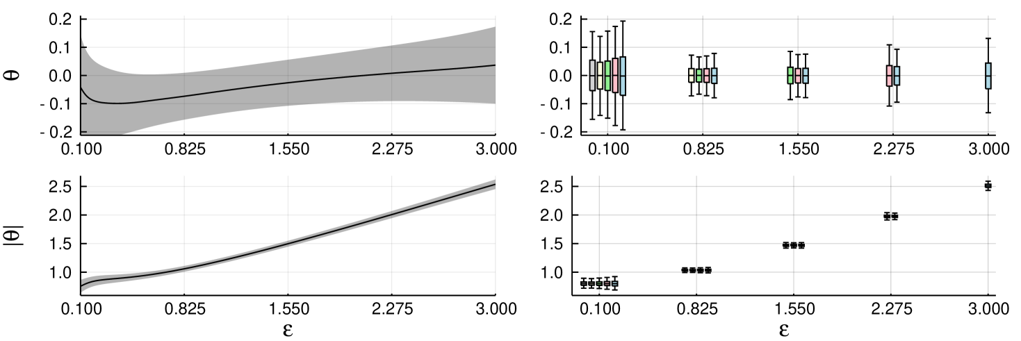
We run the experiments with 10,000 independent chains, each for 11,000 iterations including 1,000 burn-in. The chains were always started from θ0=0\theta_{0}=0. We inspect estimates for the posterior mean 𝔼πϵ[f(Θ)]\mathbb{E}_{\pi_{\epsilon}}[f(\Theta)] for f(θ)=θf(\theta)=\theta and f(θ)=|θ|f(\theta)=|\theta|. Figure 1 (left) shows the estimates with their confidence intervals based on a single realisation of abc-mcmc(3). Figure 1 (right) shows box plots of the estimates calculated from each abc-mcmc(δ\delta), with δ\delta indicated by colour; the rightmost box plot (blue) corresponds to abc-mcmc(3), the second from the right (red) abc-mcmc(2.275) etc. For ϵ=0.1\epsilon=0.1, the post-corrected estimates from abc-mcmc(0.8250.825) and abc-mcmc(1.551.55) appear slightly more accurate than direct abc-mcmc(0.10.1). Similar figure for Gaussian cut-off, with similar findings, may be found in the Supplement Figure 6.

Refer to caption
Figure 1. Gaussian model with ϕsimple\phi_{\mathrm{simple}}. Estimates from single run of abc-mcmc(33) (left) and estimates from 10,000 replications of abc-mcmc(δ\delta) for δ{0.1,0.825,1.55,2.275,3}\delta\in\{0.1,0.825,1.55,2.275,3\} indicated by colours.

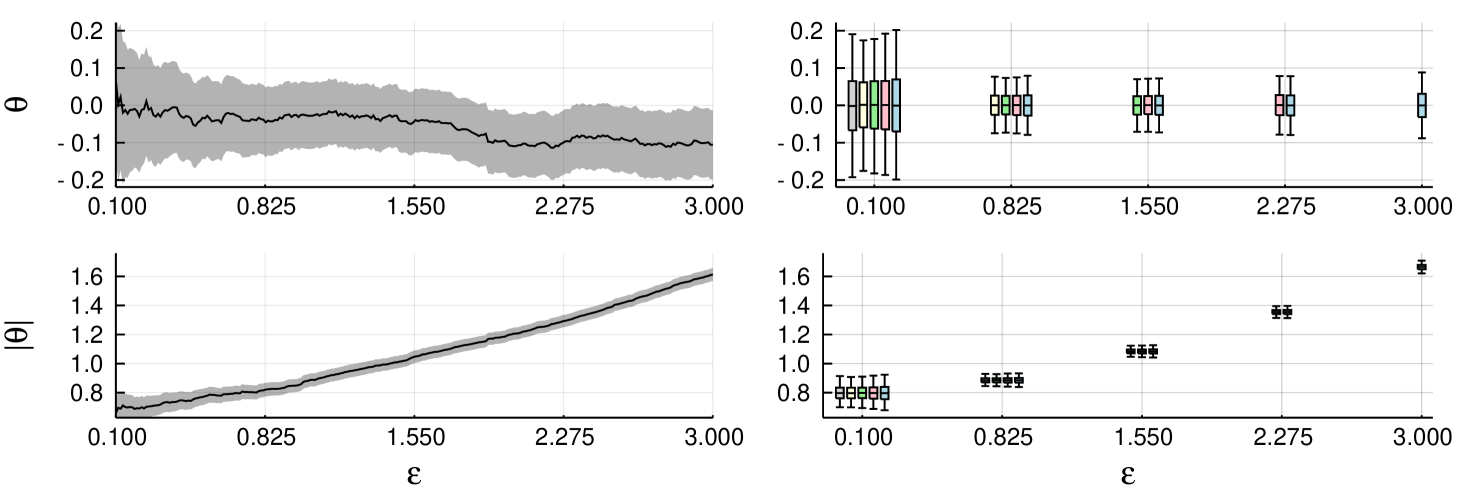
Table 1 shows frequencies of the calculated 95% confidence intervals containing the ‘ground truth’, as well as mean acceptance rates. The ground truth for 𝔼πϵ[f1(Θ)]\mathbb{E}_{\pi_{\epsilon}}[f_{1}(\Theta)] is known to be zero for all ϵ\epsilon, and the overall mean of all the calculated estimates is used as the ground truth for 𝔼πϵ[f2(Θ)]\mathbb{E}_{\pi_{\epsilon}}[f_{2}(\Theta)]. The frequencies appear close to ideal with the post-correction approach, being slightly pessimistic in case of simple cut-off as anticipated by the theoretical considerations (cf. Theorem 6 and the discussion below).

Table 1. Frequencies of the 95% confidence intervals, from abc-mcmc(δ\delta) to tolerances ϵ\epsilon, containing the ground truth in the Gaussian model.
f(x)=xf(x)=x f(x)=|x|f(x)=|x| Acc.
Cut-off δ\delta \\backslash ϵ\epsilon 0.10 0.82 1.55 2.28 3.00 0.10 0.82 1.55 2.28 3.00 rate
ϕsimple\phi_{\mathrm{simple}} 0.1 0.93 0.93 0.03
0.82 0.97 0.95 0.95 0.94 0.22
1.55 0.97 0.97 0.95 0.96 0.95 0.95 0.33
2.28 0.98 0.97 0.96 0.95 0.96 0.96 0.96 0.95 0.4
3.0 0.98 0.98 0.97 0.97 0.95 0.96 0.96 0.96 0.95 0.95 0.43
ϕGauss\phi_{\mathrm{Gauss}} 0.1 0.93 0.93 0.05
0.82 0.94 0.95 0.92 0.95 0.29
1.55 0.94 0.94 0.95 0.94 0.94 0.95 0.38
2.28 0.95 0.95 0.95 0.95 0.95 0.95 0.96 0.95 0.41
3.0 0.95 0.95 0.95 0.95 0.95 0.95 0.96 0.95 0.95 0.95 0.42

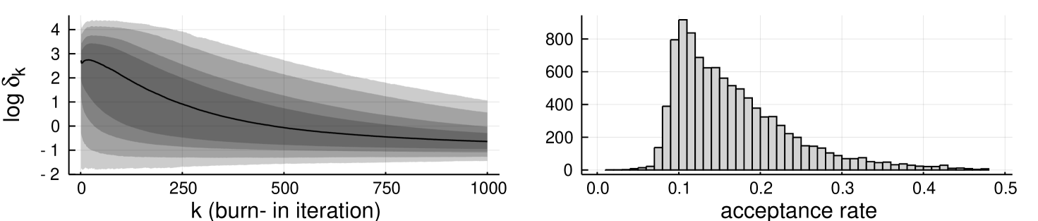
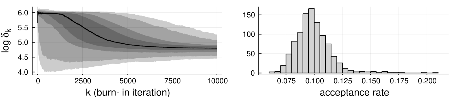
Figure 2 shows progress of tolerance adaptations during the burn-in, and histogram of the mean acceptance rates of the chain after burn-in. The lines on the left show the median, and the shaded regions indicate the 50%, 75%, 95% and 99% quantiles. The figure suggests concentration, but reveals that the adaptation has not fully converged yet. This is also visible in the mean acceptance rate over all realisations, which is 0.170.17 for simple cut-off and 0.120.12 for Gaussian cut-off (see Figure 7 in the Supplement). Table 2 shows root mean square errors for target tolerance ϵ=0.1\epsilon=0.1, with both abc-mcmc(δ\delta) with δ\delta fixed as above, and for the tolerance adaptive algorithm. Here, only the adaptive chains with final tolerance 0.1\geq 0.1 were included (9,998 and 9,993 out of 10,000 chains for ϕsimple\phi_{\mathrm{simple}} and ϕGauss\phi_{\mathrm{Gauss}}, respectively). Tolerance adaptation (started from prior distribution) appears to be competitive with ‘optimally’ tuned fixed tolerance abc-mcmc(δ\delta).

Refer to caption
Figure 2. Progress of tolerance adaptation (left) and histogram of acceptance rates (right) in the Gaussian model experiment with simple cut-off.
Table 2. Root mean square errors (×102)(\times 10^{-2}) from abc-mcmc(δ\delta) for tolerance ϵ=0.1\epsilon=0.1 with fixed tolerance and with the adaptive algorithms in the Gaussian model.
ϕsimple\phi_{\mathrm{simple}} ϕGauss\phi_{\mathrm{Gauss}}
Fixed tolerance Adapt Fixed tolerance Adapt
δ\delta 0.1 0.82 1.55 2.28 3.0 0.64 0.1 0.82 1.55 2.28 3.0 0.28
xx 9.75 8.95 9.29 9.65 10.3 9.15 7.97 7.12 7.82 8.94 9.93 7.08
|x||x| 5.49 5.35 5.51 5.81 6.24 5.38 4.47 4.22 4.68 5.26 5.95 4.15

6.2. Lotka-Volterra model

Our second experiment is a Lotka-Volterra model suggested by Boys et al. (2008), which was considered in the approximate Bayesian computation context by Fearnhead and Prangle (2012). The model is a Markov process (Xt,Yt)t0(X_{t},Y_{t})_{t\geq 0} of counts, corresponding to a reaction network X2XX\to 2X with rate θ1\theta_{1}, X+Y2YX+Y\to 2Y with rate θ2\theta_{2} and YY\to\emptyset with rate θ3\theta_{3}. The reaction log-rates (logθ1,logθ2,logθ3)T(\log\theta_{1},\log\theta_{2},\log\theta_{3})^{\mathrm{\scriptscriptstyle T}} are parameters, which we equip with a uniform prior, (logθ1,logθ2,logθ3)TU([6,0]3)(\log\theta_{1},\log\theta_{2},\log\theta_{3})^{\mathrm{\scriptscriptstyle T}}\sim U([-6,0]^{3}). The data is a simulated trajectory from the model with θ=(0.5,0.0025,0.3)T\theta=(0.5,0.0025,0.3)^{\mathrm{\scriptscriptstyle T}} until time 4040. The inference is based on the Euclidean distances of five-dimensional summary statistics of the process observed every 5 time units (X~k=X5k\tilde{X}_{k}=X_{5k} and Y~k=Y5k\tilde{Y}_{k}=Y_{5k}). The summary statistics are the sample autocorrelation of (X~k)(\tilde{X}_{k}) at lag 2 multiplied by 100, and the 10% and 90% quantiles of (X~k)(\tilde{X}_{k}) and (Y~k)(\tilde{Y}_{k}). The observed summary statistics are (51.07,29,304,65,404)T(-51.07,29,304,65,404)^{\mathrm{\scriptscriptstyle T}}.

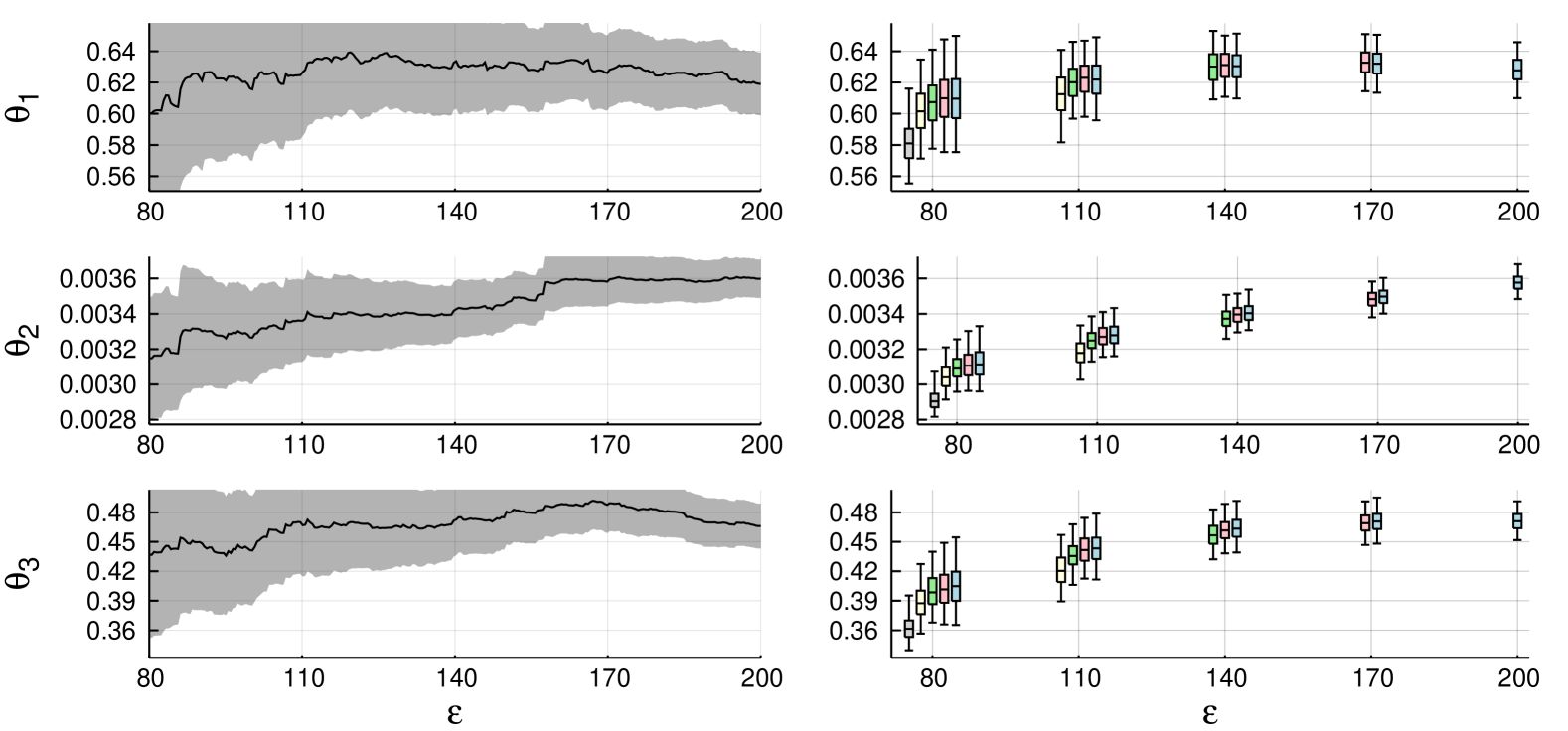
We first run comparisons similar to Section 6.1, but now with 1,000 independent abc-mcmc(δ\delta) chains with simple cut-off. We investigate the effect of post-correction, with 20,000 samples, including 10,000 burn-in, for each chain. All chains were started from near the posterior mode, from (0.55,5.77,1.09)T(-0.55,-5.77,-1.09)^{\mathrm{\scriptscriptstyle T}}. Figure 3

Refer to caption
Figure 3. Lotka-Volterra model with simple cut-off. Estimates from single run of abc-mcmc(200200) (left) and estimates from 1,000 replications of abc-mcmc(δ\delta) with δ{80,110,140,170,200}\delta\in\{80,110,140,170,200\} indicated by colour.

shows similar comparisons as in Section 6.1, and Figure 4

Refer to caption
Figure 4. Lotka-Volterra model with Epanechnikov cut-off and regression correction. Estimates from single run of abc-mcmc(200200) (left) and estimates from 1,000 replications of abc-mcmc(δ\delta) with δ{80,110,140,170,200}\delta\in\{80,110,140,170,200\} indicated by colour.

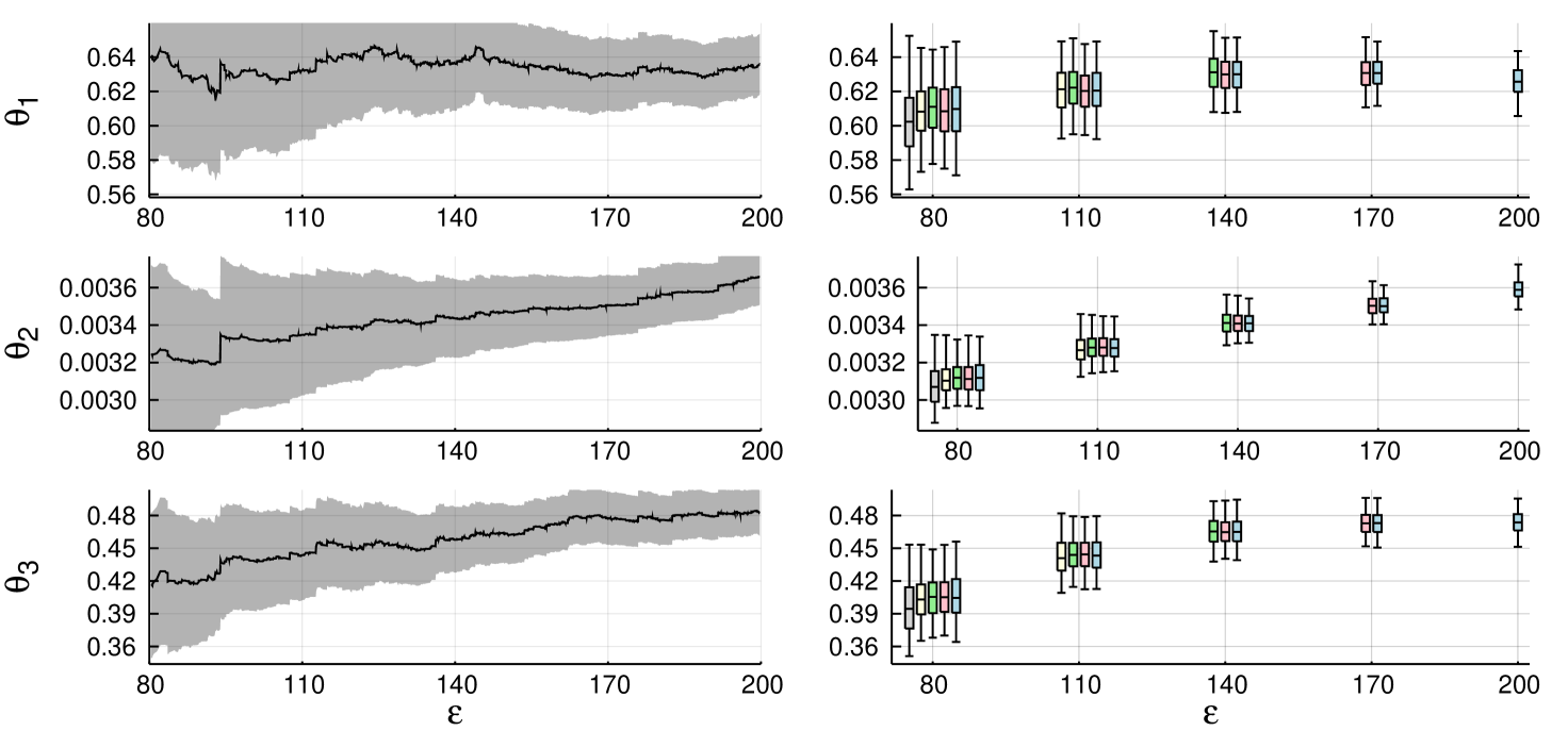
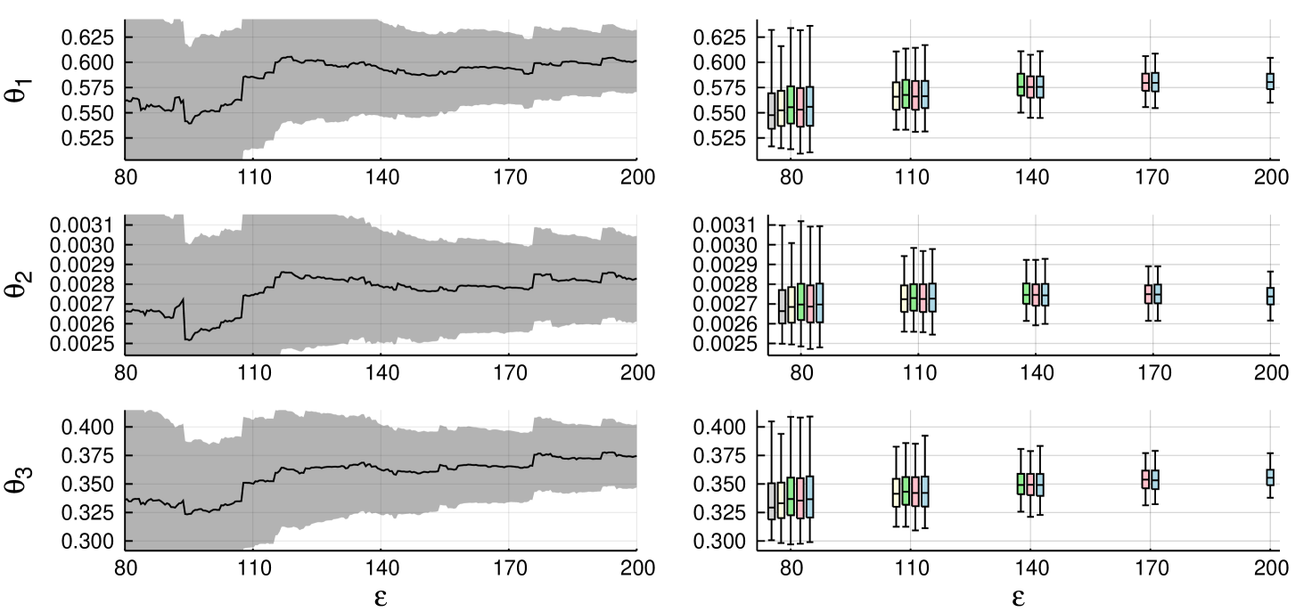
shows results for regression correction with Epanechnikov cut-off ϕEpa(t)=max{0,1t2}\phi_{\mathrm{Epa}}(t)=\max\{0,1-t^{2}\} (Beaumont et al., 2002). The results suggest that post-correction might provide slightly more accurate estimators, particularly with smaller tolerances. There is also some bias in abc-mcmc(δ\delta) with smaller δ\delta, when compared to the ground truth calculated from abc-mcmc(δ\delta) chain of ten million iterations. Table 3 shows coverages of confidence intervals.

Table 3. Mean acceptance rates and frequencies of the 95% confidence intervals, from abc-mcmc(δ\delta) to tolerances ϵ\epsilon, in the Lotka-Volterra model.
f(θ)=θ1f(\theta)=\theta_{1} f(θ)=θ2f(\theta)=\theta_{2} f(θ)=θ3f(\theta)=\theta_{3} Acc.
δ\delta \\backslash ϵ\epsilon 80 110 140 170 200 80 110 140 170 200 80 110 140 170 200 rate
ϕsimple\phi_{\mathrm{simple}} 80 0.8 0.73 0.74 0.05
110 0.97 0.93 0.94 0.89 0.94 0.9 0.07
140 0.99 0.97 0.93 0.98 0.96 0.92 0.98 0.96 0.94 0.1
170 0.99 0.98 0.96 0.93 0.98 0.97 0.96 0.93 0.99 0.98 0.96 0.95 0.14
200 1.0 0.99 0.98 0.97 0.94 0.99 0.99 0.98 0.97 0.92 0.99 0.98 0.98 0.96 0.94 0.17
regr. ϕEpa\phi_{\mathrm{Epa}} 80 0.75 0.76 0.68 0.05
110 0.92 0.92 0.93 0.94 0.87 0.91 0.07
140 0.93 0.94 0.94 0.94 0.96 0.97 0.9 0.92 0.94 0.1
170 0.93 0.95 0.95 0.95 0.96 0.97 0.97 0.98 0.92 0.94 0.94 0.95 0.14
200 0.96 0.96 0.96 0.96 0.96 0.98 0.98 0.98 0.98 0.98 0.95 0.96 0.95 0.96 0.96 0.17

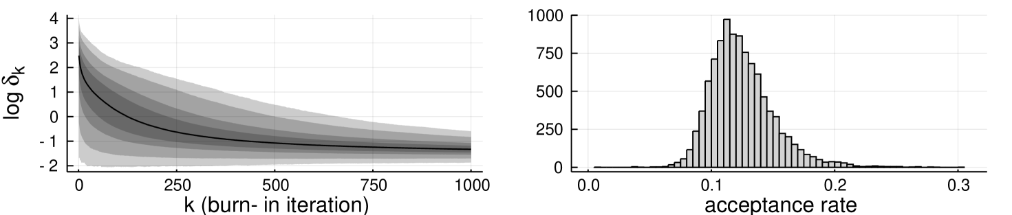
In addition, we experiment with the tolerance adaptation, using also 20,000 samples out of which 10,000 are burn-in. Figure 5

Refer to caption
Figure 5. Progress of tolerance adaptation (left) and histogram of acceptance rates (right) in the Lotka-Volterra experiment.

shows the progress of the log\log-tolerance during the burn-in, and histogram of the realised mean acceptance rates during the estimation phase. The realised acceptance rates are concentrated around the mean 0.100.10. Table 4

Table 4. Root mean square errors of estimators from abc-mcmc(δ\delta) for tolerance ϵ=80\epsilon=80, with fixed tolerance and with adaptive tolerance in the Lotka-Volterra model.
Post-correction, simple cut-off Regression, Epanechnikov cut-off
Fixed tolerance Adapt Fixed tolerance Adapt
δ\delta 80 110 140 170 200 122.6 80 110 140 170 200 122.6
θ1\theta_{1} (×102)(\times 10^{-2}) 2.37 1.81 1.75 1.83 1.93 1.8 3.1 2.74 3.02 3.09 3.19 2.57
θ2\theta_{2} (×104)(\times 10^{-4}) 1.32 0.99 0.93 0.96 1.06 1.04 1.52 1.39 1.54 1.61 1.63 1.28
θ3\theta_{3} (×102)(\times 10^{-2}) 2.94 2.26 2.11 2.14 2.37 2.34 2.77 2.53 2.76 2.85 2.91 2.34

shows root mean square errors of the estimators from abc-mcmc(δ\delta) for ϵ=80\epsilon=80 for fixed tolerance and with tolerance adaptation. Only the adaptive chains with final tolerance 80.0\geq 80.0 were included (999 out of 1,000 chains).

In this case, the chains run with the tolerance adaptation led to better results than those run only with the covariance adaptation (and fixed tolerance). This perhaps surprising result may be due to the initial behaviour of the covariance adaptation, which may be unstable when there are many rejections. Different initialisation strategies, for instance following (Haario et al., 2001, Remark 2), might lead to more stable behaviour compared to using the adaptation of Andrieu and Moulines (2006) from the start, as we do. The different step size sequences (n1n^{-1} and n2/3n^{-2/3}) could also play a rôle. We repeated the experiment for the chains with fixed tolerances, but now with covariance adaptation step size n2/3n^{-2/3}. This led to more accurate estimators for abc-mcmc(δ\delta) with higher δ\delta, but worse behaviour with smaller δ\delta. In any case, also here, tolerance adaptation delivered competitive results (see Supplement F).

7. Discussion

We believe that approximate Bayesian computation inference with Markov chain Monte Carlo is a useful approach, when the chosen simulation tolerance allows for good mixing. Our confidence intervals for post-processing and automatic tuning of simulation tolerance may make this approach more appealing in practice.

A related approach by Bortot et al. (2007) makes tolerance an auxiliary variable with a user-specified prior. This approach avoids explicit tolerance selection, but the inference is based on a pseudo-posterior πˇ(θ,δ)\check{\pi}(\theta,\delta) not directly related to πδ(θ)\pi_{\delta}(\theta) in (1). Bortot et al. (2007) also provide tolerance-dependent analysis, showing parameter means and variances with respect to conditional distributions of πˇ(θ,δ)\check{\pi}(\theta,\delta) given δϵ\delta\leq\epsilon. We believe that our approach, where the effect of tolerance in the expectations with respect πϵ\pi_{\epsilon} can be investigated explicitly, can be more immediate to interpret. Our confidence interval only shows the Monte Carlo uncertainty related to the posterior mean, and we are currently investigating how the overall parameter uncertainty could be summarised in a useful manner.

The convergence rates of approximate Bayesian computation has been investigated by Barber et al. (2015) in terms of cost and bias with respect to true posterior, and recently by Li and Fearnhead (2018a, b) in the large data limit, the latter in the context of regression. It would be interesting to consider extensions of these results in the Markov chain Monte Carlo context. In fact, Li and Fearnhead (2018a) already suggest that the acceptance rate must be lower bounded, which is in line with our adaptation rule.

Automatic selection of tolerance has been considered earlier in Ratmann et al. (2007), who propose an algorithm based on tempering and a cooling schedule. Based on our experiments, the tolerance adaptation we present in this paper appears to perform well in practice, and provides reliable results with post-correction. For the adaptation to work efficiently, the Markov chains must be taken relatively long, rendering the approach difficult for the most computationally demanding models.

We conclude with a brief discussion of certain extensions of the suggested post-correction method; more details are given in Supplement E. First, in case of non-simple cut-off, the rejected samples may be ‘recycled’ by using the acceptance probability as weight (Ceperley et al., 1977). The accuracy of the post-corrected estimator could be enhanced with smaller values of ϵ\epsilon by performing further independent simulations from g(Θk)g(\,\cdot\,\mid\Theta_{k}) (which may be calculated in parallel). The estimator is rather straightforward, but requires some care because the estimators of the pseudo-likelihood take value zero. The latter extension, which involves additional simulations as post-processing, is similar to the ‘lazy’ version of Prangle (2016, 2015) incorporating a randomised stopping rule for simulation, and to debiased ‘exact’ approach of Tran and Kohn (2015), which may lead to estimators which get rid of ϵ\epsilon-bias entirely.

8. Acknowledgements

This work was supported by Academy of Finland (grants 274740, 284513 and 312605). The authors wish to acknowledge CSC, IT Center for Science, Finland, for computational resources, and thank Christophe Andrieu for useful discussions.

References

  • Andrieu and Moulines (2006) C. Andrieu and É. Moulines. On the ergodicity properties of some adaptive MCMC algorithms. Ann. Appl. Probab., 16(3):1462–1505, 2006.
  • Andrieu and Thoms (2008) C. Andrieu and J. Thoms. A tutorial on adaptive MCMC. Statist. Comput., 18(4):343–373, Dec. 2008.
  • Andrieu et al. (2005) C. Andrieu, É. Moulines, and P. Priouret. Stability of stochastic approximation under verifiable conditions. SIAM J. Control Optim., 44(1):283–312, 2005.
  • Andrieu et al. (2018) C. Andrieu, A. Lee, and M. Vihola. Theoretical and methodological aspects of MCMC computations with noisy likelihoods. In S. A. Sisson, Y. Fan, and M. Beaumont, editors, Handbook of Approximate Bayesian Computation. Chapman & Hall/CRC Press, 2018.
  • Barber et al. (2015) S. Barber, J. Voss, and M. Webster. The rate of convergence for approximate Bayesian computation. Electron. J. Statist., 9(1):80–105, 2015.
  • Beaumont et al. (2002) M. Beaumont, W. Zhang, and D. Balding. Approximate Bayesian computation in population genetics. Genetics, 162(4):2025–2035, 2002.
  • Bezanson et al. (2017) J. Bezanson, A. Edelman, S. Karpinski, and V. B. Shah. Julia: A fresh approach to numerical computing. SIAM review, 59(1):65–98, 2017.
  • Bornn et al. (2017) L. Bornn, N. Pillai, A. Smith, and D. Woodard. The use of a single pseudo-sample in approximate Bayesian computation. Statist. Comput., 27(3):583–590, 2017.
  • Bortot et al. (2007) P. Bortot, S. Coles, and S. Sisson. Inference for stereological extremes. J. Amer. Statist. Assoc., 102(477):84–92, 2007.
  • Boys et al. (2008) R. J. Boys, D. J. Wilkinson, and T. B. Kirkwood. Bayesian inference for a discretely observed stochastic kinetic model. Stat. Comput., 18(2):125–135, 2008.
  • Burkholder et al. (1972) D. Burkholder, B. Davis, and R. Gundy. Integral inequalities for convex functions of operators on martingales. In Proc. Sixth Berkeley Symp. Math. Statist. Prob, volume 2, pages 223–240, 1972.
  • Ceperley et al. (1977) D. Ceperley, G. Chester, and M. Kalos. Monte Carlo simulation of a many-fermion study. Phys. Rev. D, 16(7):3081, 1977.
  • Delmas and Jourdain (2009) J.-F. Delmas and B. Jourdain. Does waste recycling really improve the multi-proposal Metropolis–Hastings algorithm? an analysis based on control variates. J. Appl. Probab., 46(4):938–959, 2009.
  • Doucet et al. (2015) A. Doucet, M. Pitt, G. Deligiannidis, and R. Kohn. Efficient implementation of Markov chain Monte Carlo when using an unbiased likelihood estimator. Biometrika, 102(2):295–313, 2015.
  • Fearnhead and Prangle (2012) P. Fearnhead and D. Prangle. Constructing summary statistics for approximate Bayesian computation: semi-automatic approximate Bayesian computation. J. R. Stat. Soc. Ser. B Stat. Methodol., 74(3):419–474, 2012.
  • Flegal and Jones (2010) J. M. Flegal and G. L. Jones. Batch means and spectral variance estimators in Markov chain Monte Carlo. Ann. Statist., 38(2):1034–1070, 2010.
  • Franks and Vihola (2017) J. Franks and M. Vihola. Importance sampling correction versus standard averages of reversible MCMCs in terms of the asymptotic variance. Preprint arXiv:1706.09873v3, 2017.
  • Geyer (1992) C. J. Geyer. Practical Markov chain Monte Carlo. Statist. Sci., pages 473–483, 1992.
  • Haario et al. (2001) H. Haario, E. Saksman, and J. Tamminen. An adaptive Metropolis algorithm. Bernoulli, 7(2):223–242, 2001.
  • Li and Fearnhead (2018a) W. Li and P. Fearnhead. On the asymptotic efficiency of approximate Bayesian computation estimators. Biometrika, 105(2):285–299, 2018a.
  • Li and Fearnhead (2018b) W. Li and P. Fearnhead. Convergence of regression-adjusted approximate Bayesian computation. Biometrika, 105(2):301–318, 2018b.
  • Marin et al. (2012) J.-M. Marin, P. Pudlo, C. P. Robert, and R. J. Ryder. Approximate Bayesian computational methods. Statist. Comput., 22(6):1167–1180, 2012.
  • Marjoram et al. (2003) P. Marjoram, J. Molitor, V. Plagnol, and S. Tavaré. Markov chain Monte Carlo without likelihoods. Proc. Natl. Acad. Sci. USA, 100(26):15324–15328, 2003.
  • Meyn and Tweedie (2009) S. Meyn and R. L. Tweedie. Markov Chains and Stochastic Stability. Cambridge University Press, 2nd edition, 2009. ISBN 978-0-521-73182-9.
  • Prangle (2015) D. Prangle. Lazier ABC. Preprint arXiv:1501.05144, 2015.
  • Prangle (2016) D. Prangle. Lazy ABC. Statist. Comput., 26(1-2):171–185, 2016.
  • Ratmann et al. (2007) O. Ratmann, O. Jørgensen, T. Hinkley, M. Stumpf, S. Richardson, and C. Wiuf. Using likelihood-free inference to compare evolutionary dynamics of the protein networks of H. pylori and P. falciparum. PLoS Comput. Biol., 3(11):e230, 2007.
  • Raynal et al. (to appear) L. Raynal, J.-M. Marin, P. Pudlo, M. Ribatet, C. P. Robert, and A. Estoup. ABC random forests for bayesian parameter inference. Bioinformatics, to appear.
  • Roberts et al. (1997) G. Roberts, A. Gelman, and W. Gilks. Weak convergence and optimal scaling of random walk Metropolis algorithms. Ann. Appl. Probab., 7(1):110–120, 1997.
  • Roberts and Rosenthal (2006) G. O. Roberts and J. S. Rosenthal. Harris recurrence of Metropolis-within-Gibbs and trans-dimensional Markov chains. Ann. Appl. Probab., 16(4):2123–2139, 2006.
  • Rudolf and Sprungk (2018) D. Rudolf and B. Sprungk. On a Metropolis-Hastings importance sampling estimator. Preprint arXiv:1805.07174, 2018.
  • Schuster and Klebanov (2018) I. Schuster and I. Klebanov. Markov chain importance sampling - a highly efficient estimator for MCMC. Preprint arXiv:1805.07179, 2018.
  • Sherlock et al. (2015) C. Sherlock, A. H. Thiery, G. O. Roberts, and J. S. Rosenthal. On the efficiency of pseudo-marginal random walk Metropolis algorithms. Ann. Statist., 43(1):238–275, 2015.
  • Sisson and Fan (2018) S. Sisson and Y. Fan. ABC samplers. In S. Sisson, Y. Fan, and M. Beaumont, editors, Handbook of Markov chain Monte Carlo. Chapman & Hall/CRC Press, 2018.
  • Sokal (1996) A. D. Sokal. Monte Carlo methods in statistical mechanics: Foundations and new algorithms. Lecture notes, 1996.
  • Sunnåker et al. (2013) M. Sunnåker, A. G. Busetto, E. Numminen, J. Corander, M. Foll, and C. Dessimoz. Approximate Bayesian computation. PLoS computational biology, 9(1):e1002803, 2013.
  • Tanaka et al. (2006) M. Tanaka, A. Francis, F. Luciani, and S. Sisson. Using approximate Bayesian computation to estimate tuberculosis transmission parameters from genotype data. Genetics, 173(3):1511–1520, 2006.
  • Tran and Kohn (2015) M. N. Tran and R. Kohn. Exact ABC using importance sampling. Preprint arXiv:1509.08076, 2015.
  • Vihola (2012) M. Vihola. Robust adaptive Metropolis algorithm with coerced acceptance rate. Statist. Comput., 22(5):997–1008, 2012.
  • Vihola et al. (2016) M. Vihola, J. Helske, and J. Franks. Importance sampling type estimators based on approximate marginal MCMC. Preprint arXiv:1609.02541v5, 2016.
  • Wegmann et al. (2009) D. Wegmann, C. Leuenberger, and L. Excoffier. Efficient approximate Bayesian computation coupled with Markov chain Monte Carlo without likelihoods. Genetics, 182(4):1207–1218, 2009.

Appendix

The following algorithm shows that in case of simple (post-correction) cut-off, Eδ,ϵ(f)E_{\delta,\epsilon}(f) and Sδ,ϵ(f)S_{\delta,\epsilon}(f) may be calculated simultaneously for all tolerances efficiently:

Algorithm 11.

Suppose ϕ=ϕsimple\phi=\phi_{\mathrm{simple}} and (Θk,Tk)k=1,,n(\Theta_{k},T_{k})_{k=1,\ldots,n} is the output of abc-mcmc(δ\delta).

  1. (i)

    Sort (Θk,Tk)k=1,,n(\Theta_{k},T_{k})_{k=1,\ldots,n} with respect to TkT_{k}:

    • Find indices I1,,InI_{1},\ldots,I_{n} such that TIkTIk+1T_{I_{k}}\leq T_{I_{k+1}} for all k=1,,n1k=1,\ldots,n-1.

    • Denote (Θ^k,T^k)(ΘIk,TIk)(\hat{\Theta}_{k},\hat{T}_{k})\leftarrow(\Theta_{I_{k}},T_{I_{k}}).

  2. (ii)

    For all unique values ϵ{T^1,,T^n}\epsilon\in\{\hat{T}_{1},\ldots,\hat{T}_{n}\}, let mϵ=max{k1:T^kϵ}m_{\epsilon}=\max\{k\geq 1\,:\,\hat{T}_{k}\leq\epsilon\}, and define

    Eδ,ϵ(f)=mϵ1k=1mϵf(Θ^k),andSδ,ϵ(f)=mϵ2k=1mϵ[f(Θ^k)Eδ,ϵ(f)]2.E_{\delta,\epsilon}(f)=m_{\epsilon}^{-1}\textstyle\sum_{k=1}^{m_{\epsilon}}f(\hat{\Theta}_{k}),\qquad\text{and}\qquad S_{\delta,\epsilon}(f)=m_{\epsilon}^{-2}\textstyle\sum_{k=1}^{m_{\epsilon}}\big{[}f(\hat{\Theta}_{k})-E_{\delta,\epsilon}(f)\big{]}^{2}.

    (and for T^k<ϵ<T^k+1\hat{T}_{k}<\epsilon<\hat{T}_{k+1}, let Eδ,ϵ(f)=Eδ,T^k(f)E_{\delta,\epsilon}(f)=E_{\delta,\hat{T}_{k}}(f) and Sδ,ϵ(f)=Sδ,T^k(f)S_{\delta,\epsilon}(f)=S_{\delta,\hat{T}_{k}}(f).)

The sorting in Algorithm 11(i) may be performed in O(nlogn)O(n\log n) time, and Eδ,ϵ(f)E_{\delta,\epsilon}(f) and Sδ,ϵ(f)S_{\delta,\epsilon}(f) may all be calculated in O(n)O(n) time by forming appropriate cumulative sums.

of Theorem 4.

Algorithm 1 is a Metropolis–Hastings algorithm with compound proposal q~(θ,y;θ,y)=q(θ,θ)g(yθ)\tilde{q}(\theta,y;\theta^{\prime},y^{\prime})=q(\theta,\theta^{\prime})g(y^{\prime}\mid\theta^{\prime}) and with target π~ϵ(θ,y)pr(θ)g(yθ)ϕ(d(y,y)/ϵ)\tilde{\pi}_{\epsilon}(\theta,y)\propto\mathrm{pr}(\theta)g(y\mid\theta)\phi\big{(}d(y,y^{*})/\epsilon\big{)}. The chain (Θk,Yk)k1(\Theta_{k},Y_{k})_{k\geq 1} is Harris-recurrent, as a full-dimensional Metropolis–Hastings which is φ\varphi-irreducible (Roberts and Rosenthal, 2006). Because ϕ\phi is monotone and ϵδ\epsilon\leq\delta, we have ϕ(d(y,y)/δ)ϕ(d(y,y)/ϵ)\phi\big{(}d(y,y^{*})/\delta\big{)}\geq\phi\big{(}d(y,y^{*})/\epsilon\big{)}, and therefore π~ϵ\tilde{\pi}_{\epsilon} is absolutely continuous with respect to π~δ\tilde{\pi}_{\delta}, and wδ,ϵ(y)=cδ,ϵπ~ϵ(θ,y)/π~δ(θ,y)w_{\delta,\epsilon}(y)=c_{\delta,\epsilon}\tilde{\pi}_{\epsilon}(\theta,y)/\tilde{\pi}_{\delta}(\theta,y), where cδ,ϵ>0c_{\delta,\epsilon}>0 is a constant. If we denote ξk(f)=Uk(δ,ϵ)f(Θk)\xi_{k}(f)=U_{k}^{(\delta,\epsilon)}f(\Theta_{k}) and ξk(𝟏)=Uk(δ,ϵ)=wδ,ϵ(Yk)\xi_{k}(\mathbf{1})=U_{k}^{(\delta,\epsilon)}=w_{\delta,\epsilon}(Y_{k}), then Eδ,ϵ(n)(f)=k=1nξk(f)/j=1nξj(𝟏)𝔼π~ϵ[f(Θ)]E_{\delta,\epsilon}^{(n)}(f)=\sum_{k=1}^{n}\xi_{k}(f)/\sum_{j=1}^{n}\xi_{j}(\mathbf{1})\to\mathbb{E}_{\tilde{\pi}_{\epsilon}}[f(\Theta)] almost surely by Harris recurrence and π~ϵ\tilde{\pi}_{\epsilon} invariance (e.g. Vihola et al., 2016). The claim (i) follows because πϵ\pi_{\epsilon} is the marginal density of π~ϵ\tilde{\pi}_{\epsilon}.

The chain (Θk,Yk)k1(\Theta_{k},Y_{k})_{k\geq 1} is reversible, so (ii) follows by (Vihola et al., 2016, Theorem 7(i)), because mf(2)(θ,y)=wδ,ϵ2(y)f2(θ)m_{f}^{(2)}(\theta,y)=w_{\delta,\epsilon}^{2}(y)f^{2}(\theta) satisfies

𝔼π~δ[mf(2)(Θ,Y)]=cδ,ϵ𝔼π~ϵ[wδ,ϵ(Y)f2(Θ)]cδ,ϵ𝔼πϵ[f2(Θ)]<,\mathbb{E}_{\tilde{\pi}_{\delta}}[m_{f}^{(2)}(\Theta,Y)]=c_{\delta,\epsilon}\mathbb{E}_{\tilde{\pi}_{\epsilon}}[w_{\delta,\epsilon}(Y)f^{2}(\Theta)]\leq c_{\delta,\epsilon}\mathbb{E}_{\pi_{\epsilon}}[f^{2}(\Theta)]<\infty,

and because the asymptotic variance of the function hδ,ϵh_{\delta,\epsilon} with respect to (Θk,Yk)k1(\Theta_{k},Y_{k})_{k\geq 1} may be expressed as varπ~δ(hδ,ϵ(Θ,Y))τδ,ϵ(f)\mathrm{var}_{\tilde{\pi}_{\delta}}\big{(}h_{\delta,\epsilon}(\Theta,Y)\big{)}\tau_{\delta,\epsilon}(f), so vδ,ϵ(f)=varπ~δ(hδ,ϵ(Θ,Y))/cδ,ϵ2v_{\delta,\epsilon}(f)=\mathrm{var}_{\tilde{\pi}_{\delta}}\big{(}h_{\delta,\epsilon}(\Theta,Y)\big{)}/c_{\delta,\epsilon}^{2}. The convergence nSδ,ϵ(n)(f)vδ,ϵ(f)nS_{\delta,\epsilon}^{(n)}(f)\to v_{\delta,\epsilon}(f) follows from (Vihola et al., 2016, Theorem 9). ∎

of Theorem 6.

The invariant distribution of abc-mcmc(δ\delta) may be written as π~δ(θ,y)=πδ(θ)g¯δ(yθ)\tilde{\pi}_{\delta}(\theta,y)=\pi_{\delta}(\theta)\bar{g}_{\delta}(y\mid\theta) where g¯δ(yθ)=g(yθ)1(d(y,y)δ)/Lδ(θ)\bar{g}_{\delta}(y\mid\theta)={g(y\mid\theta)}1\left(d(y,y^{*})\leq\delta\right)/L_{\delta}(\theta), and that g¯δ(yθ)wδ,ϵp(y)dy=w¯δ,ϵ(θ)\int\bar{g}_{\delta}(y\mid\theta)w_{\delta,\epsilon}^{p}(y)\mathrm{d}y=\bar{w}_{\delta,\epsilon}(\theta) for p{1,2}p\in\{1,2\}. Consequently, π~δ(hδ,ϵ)=πδ(fδ,ϵ)\tilde{\pi}_{\delta}(h_{\delta,\epsilon})=\pi_{\delta}(f_{\delta,\epsilon}) and π~δ(hδ,ϵ2)=πδ(f2w¯δ,ϵ)\tilde{\pi}_{\delta}(h_{\delta,\epsilon}^{2})=\pi_{\delta}(f^{2}\bar{w}_{\delta,\epsilon}), so varπ~δ(hδ,ϵ)=varπδ(fδ,ϵ)+πδ(w¯δ,ϵ(1w¯δ,ϵ)f2).\mathrm{var}_{\tilde{\pi}_{\delta}}(h_{\delta,\epsilon})=\mathrm{var}_{\pi_{\delta}}(f_{\delta,\epsilon})+\pi_{\delta}\big{(}\bar{w}_{\delta,\epsilon}(1-\bar{w}_{\delta,\epsilon})f^{2}\big{)}. Hereafter, let aδ,ϵ=(varπ~δ(hδ,ϵ))1/2a_{\delta,\epsilon}=\big{(}\mathrm{var}_{\tilde{\pi}_{\delta}}(h_{\delta,\epsilon})\big{)}^{-1/2} and denote h~δ,ϵ=aδ,ϵhδ,ϵ\tilde{h}_{\delta,\epsilon}=a_{\delta,\epsilon}h_{\delta,\epsilon} and f~δ,ϵ=aδ,ϵfδ,ϵ\tilde{f}_{\delta,\epsilon}=a_{\delta,\epsilon}f_{\delta,\epsilon}. Clearly, varπ~δ(h~δ,ϵ)=1\mathrm{var}_{\tilde{\pi}_{\delta}}(\tilde{h}_{\delta,\epsilon})=1 and

ρk(δ,ϵ)=ek(δ,ϵ)(πδ(f~δ,ϵ))2,whereek(δ,ϵ)=𝔼[h~δ,ϵ(Θ0(s),Y0(s))h~δ,ϵ(Θk(s),Yk(s))].\rho_{k}^{(\delta,\epsilon)}=e_{k}^{(\delta,\epsilon)}-\big{(}\pi_{\delta}(\tilde{f}_{\delta,\epsilon})\big{)}^{2},\qquad\text{where}\qquad e_{k}^{(\delta,\epsilon)}=\mathbb{E}\big{[}\tilde{h}_{\delta,\epsilon}(\Theta_{0}^{(s)},Y_{0}^{(s)})\tilde{h}_{\delta,\epsilon}(\Theta_{k}^{(s)},Y_{k}^{(s)})\big{]}.

Note that with ϕ=ϕsimple\phi=\phi_{\mathrm{simple}}, the acceptance ratio is αδ(θ,y;θ^,y^)=α˙(θ,θ^)1(d(y^,y)δ)\alpha_{\delta}(\theta,y;\hat{\theta},\hat{y})=\dot{\alpha}(\theta,\hat{\theta})1\left(d(\hat{y},y^{*})\leq\delta\right), where α˙(θ,θ^)=min{1,pr(θ^)q(θ^,θ)/(pr(θ)q(θ,θ^))},\dot{\alpha}(\theta,\hat{\theta})=\min\big{\{}1,\mathrm{pr}(\hat{\theta})q(\hat{\theta},\theta)\big{/}\big{(}\mathrm{pr}(\theta)q(\theta,\hat{\theta})\big{)}\big{\}}, which is independent of yy, so (Θk(s))(\Theta_{k}^{(s)}) is marginally a Metropolis–Hastings type chain, with proposal qq and acceptance probability α(θ,θ^)Lδ(θ^)\alpha(\theta,\hat{\theta})L_{\delta}(\hat{\theta}), and

𝔼[h~δ,ϵ(Θ1(s),Y1(s))|(Θ0(s),Y0(s))=(θ,y)]rδ(θ)h~δ,ϵ(θ,y)\displaystyle\mathbb{E}\big{[}\tilde{h}_{\delta,\epsilon}(\Theta_{1}^{(s)},Y_{1}^{(s)})\;\big{|}\;(\Theta_{0}^{(s)},Y_{0}^{(s)})=(\theta,y)\big{]}-r_{\delta}(\theta)\tilde{h}_{\delta,\epsilon}(\theta,y)
=aδ,ϵq(θ,θ^)α˙(θ,θ^)g(y^θ^)wδ,ϵ(y^)f(θ^)dθ^dy^=q(θ,θ^)α˙(θ,θ^)Lδ(θ^)f~δ,ϵ(θ^)dθ^.\displaystyle=a_{\delta,\epsilon}\int q(\theta,\hat{\theta})\dot{\alpha}(\theta,\hat{\theta})g(\hat{y}\mid\hat{\theta})w_{\delta,\epsilon}(\hat{y})f(\hat{\theta})\mathrm{d}\hat{\theta}\mathrm{d}\hat{y}=\int q(\theta,\hat{\theta})\dot{\alpha}(\theta,\hat{\theta})L_{\delta}(\hat{\theta})\tilde{f}_{\delta,\epsilon}(\hat{\theta})\mathrm{d}\hat{\theta}.

Using this iteratively, we obtain that

ek(δ,ϵ)=𝔼[f~δ,ϵ(Θ0(s))f~δ,ϵ(Θk(s))]+π~δ(θ,y)[h~δ,ϵ2(θ,y)f~δ,ϵ2(θ)]rδk(θ)dθdy,\textstyle e_{k}^{(\delta,\epsilon)}=\mathbb{E}\big{[}\tilde{f}_{\delta,\epsilon}(\Theta_{0}^{(s)})\tilde{f}_{\delta,\epsilon}(\Theta_{k}^{(s)})\big{]}+\int\tilde{\pi}_{\delta}(\theta,y)\big{[}\tilde{h}_{\delta,\epsilon}^{2}(\theta,y)-\tilde{f}_{\delta,\epsilon}^{2}(\theta)\big{]}r_{\delta}^{k}(\theta)\mathrm{d}\theta\mathrm{d}y,

and therefore with γk(δ,ϵ)=aδ,ϵ2cov(fδ,ϵ(Θ0(s)),fδ,ϵ(Θk(s)))\gamma_{k}^{(\delta,\epsilon)}=a_{\delta,\epsilon}^{2}\mathrm{cov}\big{(}f_{\delta,\epsilon}(\Theta_{0}^{(s)}),f_{\delta,\epsilon}(\Theta_{k}^{(s)})\big{)},

k1ρk(δ,ϵ)=k1γk(δ,ϵ)+aδ,ϵ2πδ(θ)w¯δ,ϵ(θ)(1w¯δ,ϵ(θ))rδ(θ)(1rδ(θ))1f2(θ)dθ.\textstyle\sum_{k\geq 1}\rho_{k}^{(\delta,\epsilon)}=\sum_{k\geq 1}\gamma_{k}^{(\delta,\epsilon)}+a_{\delta,\epsilon}^{2}\int\pi_{\delta}(\theta)\bar{w}_{\delta,\epsilon}(\theta)\big{(}1-\bar{w}_{\delta,\epsilon}(\theta)\big{)}r_{\delta}(\theta)(1-r_{\delta}(\theta))^{-1}f^{2}(\theta)\mathrm{d}\theta.

We conclude by noticing that 2k1γk(δ,ϵ)=aδ,ϵ2varπδ(fδ,ϵ)(τˇδ,ϵ(f)1)2\sum_{k\geq 1}\gamma_{k}^{(\delta,\epsilon)}=a_{\delta,\epsilon}^{2}\mathrm{var}_{\pi_{\delta}}(f_{\delta,\epsilon})(\check{\tau}_{\delta,\epsilon}(f)-1). ∎

Supplement B Convergence of the tolerance adaptive ABC-MCMC under generalised conditions

This section details a convergence theorem, under weaker assumptions than that of Theorem 10, for the tolerance adaptation (Algorithm 8) of Section 4.

For convenience, we denote the distance distribution here as TQθ()T\sim Q_{\theta}(\,\cdot\,), where T=d(Y,y)T=d(Y,y^{*}) for Yg(|θ)Y\sim g(\,\cdot\,|\theta). With this notation, and re-indexing Θk=Θ~k+1\Theta_{k}^{\prime}=\tilde{\Theta}_{k+1}, we may rewrite Algorithm 8 as follows:

Algorithm 12.

Suppose Θ0𝖳\Theta_{0}\in\mathsf{T} is a starting value with pr(Θ0)>0\mathrm{pr}(\Theta_{0})>0. Initialise δ=T0QΘ0()\delta=T_{0}\sim Q_{\Theta_{0}}(\,\cdot\,). k=0,,nb1k=0,\ldots,n_{b}-1, iterate:

  1. (i)

    Draw Θkq(Θk1,)\Theta_{k}^{\prime}\sim q(\Theta_{k-1},\,\cdot\,) and TkQΘk()T_{k}^{\prime}\sim Q_{\Theta_{k}^{\prime}}(\,\cdot\,).

  2. (ii)

    Accept, by setting (Θk+1,Tk+1)(Θk,Tk)(\Theta_{k+1},T_{k+1})\leftarrow(\Theta_{k}^{\prime},T_{k}^{\prime}), with probability

    (2) αδk(Θk,Tk;Θk,Tk)=min{1,pr(Θk)q(Θk,Θk)ϕ(Tk/δk)pr(Θk)q(Θk,Θk)ϕ(Tk/δk)}\alpha_{\delta_{k}}^{\prime}(\Theta_{k},T_{k};\Theta_{k}^{\prime},T_{k}^{\prime})=\min\bigg{\{}1,\frac{\mathrm{pr}(\Theta_{k}^{\prime})q(\Theta_{k}^{\prime},\Theta_{k})\phi(T_{k}^{\prime}/\delta_{k})}{\mathrm{pr}(\Theta_{k})q(\Theta_{k},\Theta_{k}^{\prime})\phi(T_{k}/\delta_{k})}\bigg{\}}

    and otherwise reject, by setting (Θk+1,Tk+1)(Θk,Tk)(\Theta_{k+1},T_{k+1})\leftarrow(\Theta_{k},T_{k}).

  3. (iii)

    logδk+1logδk+γk+1(ααδk(Θk,Θk,Tk))\log\delta_{k+1}\leftarrow\log\delta_{k}+\gamma_{k+1}\big{(}\alpha^{*}-\alpha_{\delta_{k}}^{\prime}(\Theta_{k},\Theta_{k}^{\prime},T_{k}^{\prime})\big{)}.

Let us set β=logδ\beta=\log\delta, and consider the proposal-rejection Markov kernel

(3) P˙β(θ,dϑ)=q(θ,dϑ)αβ(θ,ϑ)+(1q(θ,dϑ)αβ(θ,ϑ))1(θdϑ),\dot{P}_{\beta}(\theta,\mathrm{d}\vartheta)=q(\theta,\mathrm{d}\vartheta)\alpha_{\beta}(\theta,\vartheta)+\bigg{(}1-\int q(\theta,\mathrm{d}\vartheta)\alpha_{\beta}(\theta,\vartheta)\bigg{)}1\left(\theta\in\mathrm{d}\vartheta\right),

where αβ(θ,ϑ)=α˙(θ,ϑ)Lβ(ϑ),\alpha_{\beta}(\theta,\vartheta)=\dot{\alpha}(\theta,\vartheta)L_{\beta}(\vartheta),

α˙(θ,ϑ)=min{1,pr(ϑ)q(ϑ,θ)pr(θ)q(θ,ϑ)},andLβ(ϑ)=Qϑ(dt)1(teβ).\dot{\alpha}(\theta,\vartheta)=\min\bigg{\{}1,\frac{\mathrm{pr}(\vartheta)q(\vartheta,\theta)}{\mathrm{pr}(\theta)q(\theta,\vartheta)}\bigg{\}},\qquad\text{and}\qquad L_{\beta}(\vartheta)=\int Q_{\vartheta}(\mathrm{d}t)1\left(t\leq e^{\beta}\right).

Then P˙βk\dot{P}_{\beta_{k}} is the transition of the θ\theta-coordinate chain of Algorithm 12 with simple cut-off at iteration kk, obtained by disregarding the tt-coordinate. It is easily seen to be reversible with respect to the posterior probability πβ(θ)pr(θ)Lβ(θ)\pi_{\beta}(\theta)\propto\mathrm{pr}(\theta)L_{\beta}(\theta) given in (1), written here in terms of β=logδ\beta=\log\delta instead of δ\delta.

Assumption 13.

Suppose ϕ=ϕsimple\phi=\phi_{\mathrm{simple}} and the following hold:

  1. (i)

    Step sizes (γk)k1(\gamma_{k})_{k\geq 1} satisfy γk0\gamma_{k}\geq 0, γk+1γk\gamma_{k+1}\leq\gamma_{k},

    k1γk=,andk1γk2(1+|logγk|+|logγk|2)<.\sum_{k\geq 1}\gamma_{k}=\infty,\qquad\text{and}\qquad\sum_{k\geq 1}\gamma_{k}^{2}\Big{(}1+\lvert\log\gamma_{k}\rvert+\lvert\log\gamma_{k}\rvert^{2}\Big{)}<\infty.
  2. (ii)

    The domain 𝖳nθ\mathsf{T}\subset\mathbb{R}^{n_{\theta}}, nθ1n_{\theta}\geq 1, is a nonempty open set.

  3. (iii)

    pr()\mathrm{pr}(\,\cdot\,) and q(θ,)q(\theta,\,\cdot\,) are uniformly bounded densities on nθ\mathbb{R}^{n_{\theta}} (i.e. C>0\exists C>0 s.t. q(θ,ϑ)<Cq(\theta,\vartheta)<C and pr(θ)<C\mathrm{pr}(\theta)<C for all θ,ϑnθ\theta,\,\vartheta\in\mathbb{R}^{n_{\theta}}), and pr(θ)=0\mathrm{pr}(\theta)=0 for θ𝖳\theta\notin\mathsf{T}.

  4. (iv)

    Qθ(dt)Q_{\theta}(\mathrm{d}t) admits a uniformly bounded density Qθ(t)Q_{\theta}(t).

  5. (v)

    The values {βk}\{\beta_{k}\} remain in some compact subset 𝖡\mathsf{B}\subset\mathbb{R} almost surely.

  6. (vi)

    cβ>0c_{\beta}>0 for all β𝖡\beta\in\mathsf{B}, where cβ=pr(dθ)Lβ(θ)c_{\beta}=\int\mathrm{pr}(\mathrm{d}\theta)L_{\beta}(\theta).

  7. (vii)

    There exists V˙:𝖳[1,)\dot{V}:\mathsf{T}\to[1,\infty) such that the Markov transitions P˙β\dot{P}_{\beta} are simultaneously V˙\dot{V}-geometrically ergodic: there exist C>0C>0 and ρ(0,1)\rho\in(0,1) s.t. for all k1k\geq 1 and f:𝖳f:\mathsf{T}\to\mathbb{R} with |f|V˙\lvert f\rvert\leq\dot{V}, it holds that

    |P˙βkf(θ)πβ(f)|CV˙(θ)ρk.\lvert\dot{P}_{\beta}^{k}f(\theta)-\pi_{\beta}(f)\rvert\leq C\dot{V}(\theta)\rho^{k}.
  8. (viii)

    With 𝔼[]=𝔼θ,β[]\mathbb{E}[\,\cdot\,]=\mathbb{E}_{\theta,\beta}[\,\cdot\,] denoting expectation with respect to the law of the marginal chain (Θk)(\Theta_{k}) of Algorithm 12 started at θ𝖳\theta\in\mathsf{T}, β𝖡\beta\in\mathsf{B}, and with V˙\dot{V} as in Assumption 13(vii), we have,

    supθ,β,k𝔼[V˙(Θk)2]<.\sup_{\theta,\beta,k}\mathbb{E}\big{[}\dot{V}(\Theta_{k})^{2}\big{]}<\infty.
Theorem 14.

Under Assumption 13, the expected value of the acceptance probability (2), taken with respect to the stationary measure of the chain, converges to α\alpha^{*}.

Proof of Theorem 14 can be found in Section C. It relies heavily on the simple conditions of (Andrieu et al., 2005, Theorem 2.3), which says that one must essentially show that the noise in the stochastic approximation update is asymptotically controlled.

We remark that there are likely extensions of Assumption 13(v) to the general non-compact adaptation parameter case based on projections (cf. Andrieu et al., 2005).

Supplement C Analysis of the tolerance adaptive ABC-MCMC

In this section we aim to prove generalised convergence (Theorem 14 of Section B) of the tolerance adaptation, from which Theorem 10 of Section 4 will follow as a corollary. Throughout, we denote by C>0C>0 a constant which may change from line to line.

C.1. Proposal augmentation

Suppose L˙\dot{L} is a Markov kernel which can be written as

(4) L˙(x,dy)=q(x,dy)α(x,y)+(1q(x,dy)α(x,y))1(xdy),\dot{L}(x,\mathrm{d}y)=q(x,\mathrm{d}y)\alpha(x,y)+\bigg{(}1-\int q(x,\mathrm{d}y^{\prime})\alpha(x,y^{\prime})\bigg{)}1\left(x\in\mathrm{d}y\right),

where α(x,y)[0,1]\alpha(x,y)\in[0,1] is a jointly measurable function and q(x,dy)q(x,\mathrm{d}y) is a Markov proposal kernel. With x˘=(x,x)\breve{x}=(x,x^{\prime}), we define the proposal augmentation to be the Markov kernel

(5) L(x˘,dy˘)=α(x˘)1(xdy)q(x,dy)+(1α(x˘))1(xdy)q(x,dy).L(\breve{x},\mathrm{d}\breve{y})=\alpha(\breve{x})1\left(x^{\prime}\in\mathrm{d}y\right)q(x^{\prime},\mathrm{d}y^{\prime})+\big{(}1-\alpha(\breve{x})\big{)}1\left(x\in\mathrm{d}y\right)q(x,\mathrm{d}y^{\prime}).

It is easy to see that LL need not be reversible even if L˙\dot{L} is reversible. In this case, however, LL does leave a probability measure invariant.

Lemma 15.

Suppose a Markov kernel L˙\dot{L} of the form given in (4) is μ˙\dot{\mu}-reversible. Let LL be its proposal augmentation. Then the following statements hold:

  1. (i)

    μL=μ\mu L=\mu, where μ(dx,dx)=μ˙(dx)q(x,dx)\mu(\mathrm{d}x,\mathrm{d}x^{\prime})=\dot{\mu}(\mathrm{d}x)q(x,\mathrm{d}x^{\prime}).

  2. (ii)

    If L˙\dot{L} is V˙\dot{V}-geometrically ergodic with constants (C˙,ρ˙)(\dot{C},\dot{\rho}), then LL is VV-geometrically ergodic with constants (C,ρ)(C,\rho), where C=2C˙/ρ˙,C=2\dot{C}/\dot{\rho}, ρ=ρ˙,\rho=\dot{\rho}, and V(x˘)=12(V(x)+V(x)).V(\breve{x})=\frac{1}{2}\big{(}V(x)+V(x^{\prime})\big{)}.

Lemma 15 extends (Schuster and Klebanov, 2018, Theorem 4), who consider the case where P˙\dot{P} is a Metropolis–Hastings chain (see also Delmas and Jourdain, 2009; Rudolf and Sprungk, 2018). The extension to the more general class of reversible proposal-rejection chains allows one to consider, for example, jump and delayed acceptance chains, as well as the marginal chain (3) of Section B, which will be important for our analysis of the tolerance adaptation.

of Lemma 15.

Part (i) follows by a direct calculation. We now consider part (ii). For f:𝖷2f:\mathsf{X}^{2}\to\mathbb{R}, we shall use the notation f˙(x)=f(x˘)q(x,dx).\dot{f}(x)=\int f(\breve{x})q(x,\mathrm{d}x^{\prime}). For f:𝖷2f:\mathsf{X}^{2}\to\mathbb{R}, we have

q(x,dx)L((x,x);dy˘)f(y˘)=q(x,dx)α(x˘)f˙(x)+q(x,dx)(1α(x˘))f˙(x)=L˙f˙(x),\int q(x,\mathrm{d}x^{\prime})L\big{(}(x,x^{\prime});\mathrm{d}\breve{y}\big{)}f(\breve{y})=\int q(x,\mathrm{d}x^{\prime})\alpha(\breve{x})\dot{f}(x^{\prime})+\int q(x,\mathrm{d}x^{\prime})\big{(}1-\alpha(\breve{x})\big{)}\dot{f}(x)=\dot{L}\dot{f}(x),

and then inductively, for k1k\geq 1,

q(x,dx)Lk((x,x);dy˘)f(y˘)\displaystyle\int q(x,\mathrm{d}x^{\prime})L^{k}\big{(}(x,x^{\prime});\mathrm{d}\breve{y}\big{)}f(\breve{y}) =q(x,dx)α(x˘)q(x,dy)Lk1((x,y);dz˘)f(z˘)\displaystyle=\int q(x,\mathrm{d}x^{\prime})\alpha(\breve{x})q(x^{\prime},\mathrm{d}y^{\prime})L^{k-1}\big{(}(x^{\prime},y^{\prime});\mathrm{d}\breve{z}\big{)}f(\breve{z})
+q(x,dx)(1α(x˘))q(x,dy)Lk1((x,y);dz˘)f(z˘)\displaystyle\qquad+\int q(x,\mathrm{d}x^{\prime})\big{(}1-\alpha(\breve{x})\big{)}q(x,\mathrm{d}y^{\prime})L^{k-1}\big{(}(x,y^{\prime});\mathrm{d}\breve{z})f(\breve{z})
=q(x,dx)α(x˘)L˙k1f˙(x)+q(x,dx)(1α(x˘))L˙k1f˙(x)\displaystyle=\int q(x,\mathrm{d}x^{\prime})\alpha(\breve{x})\dot{L}^{k-1}\dot{f}(x^{\prime})+\int q(x,\mathrm{d}x^{\prime})\big{(}1-\alpha(\breve{x})\big{)}\dot{L}^{k-1}\dot{f}(x)
=L˙kf˙(x).\displaystyle=\dot{L}^{k}\dot{f}(x).

We then have the equality,

Lkf(x˘)\displaystyle L^{k}f(\breve{x}) =α(x˘)q(x,dy)Lk1((x,y);dz˘)f(z˘)+(1α(x˘))q(x,dy)Lk1((x,y);dz˘)f(z˘)\displaystyle=\alpha(\breve{x})\int q(x^{\prime},\mathrm{d}y^{\prime})L^{k-1}\big{(}(x^{\prime},y^{\prime});\mathrm{d}\breve{z}\big{)}f(\breve{z})+\big{(}1-\alpha(\breve{x})\big{)}\int q(x,\mathrm{d}y^{\prime})L^{k-1}\big{(}(x,y^{\prime});\mathrm{d}\breve{z}\big{)}f(\breve{z})
=α(x˘)L˙k1f˙(x)+(1α(x˘))L˙k1f˙(x).\displaystyle=\alpha(\breve{x})\dot{L}^{k-1}\dot{f}(x^{\prime})+\big{(}1-\alpha(\breve{x})\big{)}\dot{L}^{k-1}\dot{f}(x).

For fV\lVert f\rVert\leq V, note that f˙V˙\lVert\dot{f}\rVert\leq\dot{V} since q1\lVert q\rVert_{\infty}\leq 1, and we conclude (ii) from

|Lkf(x˘)μ(f)|\displaystyle\lvert L^{k}f(\breve{x})-\mu(f)\rvert α(x˘)|L˙k1f˙(x)μ˙(f˙)|+(1α(x˘))|L˙k1f˙(x)μ˙(f˙)|\displaystyle\leq\alpha(\breve{x})\lvert\dot{L}^{k-1}\dot{f}(x^{\prime})-\dot{\mu}(\dot{f})\rvert+\big{(}1-\alpha(\breve{x})\big{)}\lvert\dot{L}^{k-1}\dot{f}(x)-\dot{\mu}(\dot{f})\rvert
C˙ρ˙k1(V˙(x)+V˙(x)).\displaystyle\leq\dot{C}\dot{\rho}^{k-1}\big{(}\dot{V}(x^{\prime})+\dot{V}(x)\big{)}.\qed

Consider now the θ\theta-coordinate chain P˙β\dot{P}_{\beta} presented in (3) of Section B. This transition P˙β\dot{P}_{\beta} is clearly a reversible proposal-rejection chain of the form (4). We now consider PβP_{\beta}, its proposal augmentation. This is the chain Θ˘k=(Θk,Θk)𝖳2\breve{\Theta}_{k}=(\Theta_{k},\Theta_{k}^{\prime})\in{\mathsf{T}}^{2}, formed by disregarding the tt-parameter as with P˙β\dot{P}_{\beta} before, but now augmenting by the proposal θq(θ,)\theta^{\prime}\sim q(\theta,\,\cdot\,). Its transitions are of the form θ˘=Θ˘k\breve{\theta}=\breve{\Theta}_{k} goes to ϑ˘=Θ˘k+1\breve{\vartheta}=\breve{\Theta}_{k+1} in the ABC-MCMC, with ϑ˘=(ϑ,ϑ)\breve{\vartheta}=(\vartheta,\vartheta^{\prime}) and kernel

Pβ(θ˘,dϑ˘)=αβ(θ˘)1(θdϑ)q(θ,dϑ)+(1αβ(θ˘))1(θdϑ)q(θ,dϑ)P_{\beta}(\breve{\theta},\mathrm{d}\breve{\vartheta})=\alpha_{\beta}(\breve{\theta})1\left(\theta^{\prime}\in\mathrm{d}\vartheta\right)q(\theta^{\prime},\mathrm{d}\vartheta^{\prime})+\big{(}1-\alpha_{\beta}(\breve{\theta})\big{)}1\left(\theta\in\mathrm{d}\vartheta\right)q(\theta,\mathrm{d}\vartheta^{\prime})

By Lemma 15(i), PβP_{\beta} leaves πβ=πβ,u/cβ\pi_{\beta}^{\prime}=\pi_{\beta,u}^{\prime}/c_{\beta} invariant, where πβ,u(dθ˘)=pr(dθ)Lβ(θ)q(θ,dθ)\pi_{\beta,u}^{\prime}(\mathrm{d}\breve{\theta})=\mathrm{pr}(\mathrm{d}\theta)L_{\beta}(\theta)q(\theta,\mathrm{d}\theta^{\prime}) and cβ=pr(dθ)Lβ(θ).c_{\beta}=\int\mathrm{pr}(\mathrm{d}\theta)L_{\beta}(\theta).

C.2. Monotonicity properties

The following result establishes monotonicity of the mean field acceptance rate with increasing tolerance.

Lemma 16.

Assume Assumption 13(iii) and 13(iv) hold. The mapping βπβ(αβ)\beta\mapsto\pi_{\beta}^{\prime}(\alpha_{\beta}) is monotone non-decreasing.

Proof.

Since pr(θ)\mathrm{pr}(\theta) and q(θ,θ)q(\theta,\theta^{\prime}) are uniformly bounded (Assumption 13(iii)), and Lβ(θ)1L_{\beta}(\theta)\leq 1, differentiation under the integral sign is possible in the following by the dominated convergence theorem. By the quotient rule,

(6) ddβ(πβ(αβ))=1cβ2(cβddβ(πβ,u(αβ))πβ,u(αβ)dcβdβ).\frac{\mathrm{d}}{\mathrm{d}\beta}\Big{(}\pi_{\beta}^{\prime}(\alpha_{\beta})\Big{)}=\frac{1}{c_{\beta}^{2}}\bigg{(}c_{\beta}\frac{\mathrm{d}}{\mathrm{d}\beta}\Big{(}\pi_{\beta,u}^{\prime}(\alpha_{\beta})\Big{)}-\pi_{\beta,u}^{\prime}(\alpha_{\beta})\frac{\mathrm{d}c_{\beta}}{\mathrm{d}\beta}\bigg{)}.

By reversibility of Metropolis–Hastings targeting pr(θ)\mathrm{pr}(\theta) with proposal qq,

ddβ(πβ,u(αβ))=2eβpr(dθ)Lβ(θ)q(θ,dθ)α˙(θ,θ)Qθ(eβ).\frac{\mathrm{d}}{\mathrm{d}\beta}\Big{(}\pi_{\beta,u}^{\prime}(\alpha_{\beta})\Big{)}=2e^{\beta}\int\mathrm{pr}(\mathrm{d}\theta)L_{\beta}(\theta)q(\theta,\mathrm{d}\theta^{\prime})\dot{\alpha}(\theta,\theta^{\prime})Q_{\theta^{\prime}}(e^{\beta}).

With

f(θ)=2Qθ(eβ)pr(dθ~)Lβ(θ~)Lβ(θ)pr(dθ~)Qθ~(eβ),f(\theta^{\prime})=2Q_{\theta^{\prime}}(e^{\beta})\int\mathrm{pr}(\mathrm{d}\tilde{\theta})L_{\beta}(\tilde{\theta})-L_{\beta}(\theta^{\prime})\int\mathrm{pr}(\mathrm{d}\tilde{\theta})Q_{\tilde{\theta}}(e^{\beta}),

we can then write (6) as

ddβ(πβ(αβ))=eβcβ2pr(dθ)Lβ(θ)q(θ,dθ)α˙(θ,θ)f(θ).\frac{\mathrm{d}}{\mathrm{d}\beta}\Big{(}\pi_{\beta}^{\prime}(\alpha_{\beta})\Big{)}=\frac{e^{\beta}}{c_{\beta}^{2}}\int\mathrm{pr}(\mathrm{d}\theta)L_{\beta}(\theta)q(\theta,\mathrm{d}\theta^{\prime})\dot{\alpha}(\theta,\theta^{\prime})f(\theta^{\prime}).

By the same reversibility property as before, we can write this again as

ddβ(πβ(αβ))=eβcβ2f(θ)pr(dθ)q(θ,dθ)Lβ(θ)α˙(θ,θ),\frac{\mathrm{d}}{\mathrm{d}\beta}\Big{(}\pi_{\beta}^{\prime}(\alpha_{\beta})\Big{)}=\frac{e^{\beta}}{c_{\beta}^{2}}\int f(\theta)\mathrm{pr}(\mathrm{d}\theta)\int q(\theta,\mathrm{d}\theta^{\prime})L_{\beta}(\theta^{\prime})\dot{\alpha}(\theta,\theta^{\prime}),

We then conclude, since

f(θ)pr(dθ)=Qθ(eβ)pr(dθ)Lβ(θ~)pr(dθ~)0.\int f(\theta)\mathrm{pr}(\mathrm{d}\theta)=\int Q_{\theta}(e^{\beta})\mathrm{pr}(\mathrm{d}\theta)\int L_{\beta}(\tilde{\theta})\mathrm{pr}(\mathrm{d}\tilde{\theta})\geq 0.\qed
Lemma 17.

The following statements hold:

  1. (i)

    The function βcβ\beta\mapsto c_{\beta} is monotone non-decreasing on \mathbb{R}.

  2. (ii)

    If Assumption 13(v) and 13(vi) hold, then there exist Cmin>0C_{\min}>0, Cmax>0C_{\max}>0 such that CmincβCmaxC_{\min}\leq c_{\beta}\leq C_{\max} for all β𝖡\beta\in\mathsf{B}.

Proof.

Part (i) follows, for ββ\beta\leq\beta^{\prime}, from

cβ=pr(dθ)Qθ([0,eβ])pr(dθ)Qθ([0,eβ])=cβ.c_{\beta}=\int\mathrm{pr}(\mathrm{d}\theta)Q_{\theta}([0,e^{\beta}])\leq\int\mathrm{pr}(\mathrm{d}\theta)Q_{\theta}([0,e^{\beta^{\prime}}])=c_{\beta^{\prime}}.

Consider part (ii). By part (i) and compactness of 𝖡\mathsf{B} (Assumption 13(v)), we can set Cmin=cmin(𝖡)C_{\min}=c_{\min(\mathsf{B})} and Cmax=cmax(𝖡),C_{\max}=c_{\max(\mathsf{B})}, both of which are positive by Assumption 13(vi). ∎

C.3. Stochastic approximation framework

To obtain a form common in the stochastic approximation literature (cf. Andrieu et al., 2005), we write the update in Algorithm 12 as

βk+1\displaystyle\beta_{k+1} =βk+γk+1Hβk(Θ˘k,Tk)\displaystyle=\beta_{k}+\gamma_{k+1}H_{\beta_{k}}(\breve{\Theta}_{k},T_{k}^{\prime})
=βk+γk+1h(βk)+γk+1ζk+1\displaystyle=\beta_{k}+\gamma_{k+1}h(\beta_{k})+\gamma_{k+1}\zeta_{k+1}

where Hβ(θ˘,t)=ααβ(θ˘,t),H_{\beta}(\breve{\theta},t^{\prime})=\alpha^{*}-\alpha_{\beta}^{\prime}(\breve{\theta},t^{\prime}),

αβ(θ˘,t)=min{1,pr(θ)q(θ,θ)pr(θ)q(θ,θ)}1(teβ),\alpha_{\beta}^{\prime}(\breve{\theta},t^{\prime})=\min\bigg{\{}1,\frac{\mathrm{pr}(\theta^{\prime})q(\theta^{\prime},\theta)}{\mathrm{pr}(\theta)q(\theta,\theta^{\prime})}\bigg{\}}1\left(t^{\prime}\leq e^{\beta}\right),
h(β)=πβ(H^β)=πβ(dθ)q(θ,dθ)Qθ(dt)Hβ(θ,θ,t),h(\beta)=\pi_{\beta}^{\prime}(\widehat{H}_{\beta})=\int\pi_{\beta}(\mathrm{d}\theta)q(\theta,\mathrm{d}\theta^{\prime})Q_{\theta^{\prime}}(\mathrm{d}t^{\prime})H_{\beta}(\theta,\theta^{\prime},t^{\prime}),

noise sequence ζk+1=Hβk(Θ˘k,Tk)h(βk),\zeta_{k+1}=H_{\beta_{k}}(\breve{\Theta}_{k},T_{k}^{\prime})-h(\beta_{k}), and conditional expectation

H^β(θ˘)=𝔼[Hβ(Θ˘,T)|Θ˘=θ˘],\widehat{H}_{\beta}(\breve{\theta})=\mathbb{E}[H_{\beta}(\breve{\Theta},T^{\prime})|\breve{\Theta}=\breve{\theta}],

where TQθ()T^{\prime}\sim Q_{\theta^{\prime}}(\,\cdot\,). We also set for convenience H¯β(θ˘)=H^β(θ˘)πβ(H^β).\bar{H}_{\beta}(\breve{\theta})=\widehat{H}_{\beta}(\breve{\theta})-\pi_{\beta}^{\prime}(\widehat{H}_{\beta}).

Lemma 18.

Suppose Assumption 13(vii) holds. Then the following statements hold:

  1. (i)

    The proposal augmented kernels (Pβ)β𝖡(P_{\beta})_{\beta\in\mathsf{B}} are simultaneously VV-geometrically ergodic, where V(θ,θ)=12(V˙(θ)+V˙(θ))V(\theta,\theta^{\prime})=\frac{1}{2}\big{(}\dot{V}(\theta)+\dot{V}(\theta^{\prime})\big{)}, with V˙\dot{V} as in Assumption 13(vii).

  2. (ii)

    There exists C>0C>0, such that for all β𝖡\beta\in\mathsf{B}, the formal solution gβ=k0PβkH¯βg_{\beta}=\sum_{k\geq 0}P_{\beta}^{k}\bar{H}_{\beta} to the Poisson equation gβPβgβ=H¯βg_{\beta}-P_{\beta}g_{\beta}=\bar{H}_{\beta} satisfies |gβ(θ˘)|CV(θ˘).\lvert g_{\beta}(\breve{\theta})\rvert\leq CV(\breve{\theta}).

Proof.

(i) follows directly from the explicit parametrisation for (C,ρ)(C,\rho) given in Lemma 15(ii).

Part (ii) follows from part (i) and the bound, since |H¯β|1V\lvert\bar{H}_{\beta}\rvert\leq 1\leq V,

|gβ(θ˘)|1+Cβk1ρβkV(θ˘)(1+Cβ1ρβ)V(θ˘).\lvert g_{\beta}(\breve{\theta})\rvert\leq 1+C_{\beta}\sum_{k\geq 1}\rho_{\beta}^{k}V(\breve{\theta})\leq\bigg{(}1+\frac{C_{\beta}}{1-\rho_{\beta}}\bigg{)}V(\breve{\theta}).\qed

C.4. Contractions

We define for V:𝖳[1,)V:\mathsf{T}\rightarrow[1,\infty) and g:𝖳g:\mathsf{T}\to\mathbb{R} the VV-norm gV=supθ𝖳|g(θ)|V(θ).\lVert g\rVert_{V}=\sup_{\theta\in\mathsf{T}}\frac{|g(\theta)|}{V(\theta)}. We define for a bounded operator AA on a Banach space of bounded functions ff, the operator norm A=supfAff\lVert A\rVert_{\infty}=\sup_{f}\frac{\lVert Af\rVert_{\infty}}{\lVert f\rVert_{\infty}}.

Lemma 19.

Suppose Assumption 13(iv), 13(v) and 13(vi) hold. The following hold:

  1. (i)

    C>0\exists C>0, C𝖡+>0\exists C_{\mathsf{B}}^{+}>0 s.t. β1𝖡\forall\beta_{1}\in\mathsf{B}, β2𝖡\forall\beta_{2}\in\mathsf{B}, g:𝖳2\forall g:\mathsf{T}^{2}\to\mathbb{R} bounded, we have

    (Pβ1Pβ2)gCg|eβ1eβ2|C𝖡+g|β1β2|.\lVert(P_{\beta_{1}}-P_{\beta_{2}})g\rVert_{\infty}\leq C\lVert g\rVert_{\infty}\lvert e^{\beta_{1}}-e^{\beta_{2}}\rvert\leq C_{\mathsf{B}}^{+}\lVert g\rVert_{\infty}\lvert\beta_{1}-\beta_{2}\rvert.
  2. (ii)

    C𝖡>0\exists C_{\mathsf{B}}^{-}>0, C𝖡>0\exists C_{\mathsf{B}}>0, s.t. β1𝖡\forall\beta_{1}\in\mathsf{B}, β2𝖡\forall\beta_{2}\in\mathsf{B}, we have

    H¯β1H¯β2C𝖡|eβ1eβ2|C𝖡|β1β2|.\lVert\bar{H}_{\beta_{1}}-\bar{H}_{\beta_{2}}\rVert_{\infty}\leq C_{\mathsf{B}}^{-}\lvert e^{\beta_{1}}-e^{\beta_{2}}\rvert\leq C_{\mathsf{B}}\lvert\beta_{1}-\beta_{2}\rvert.
  3. (iii)

    C𝖡>0\exists C_{\mathsf{B}}^{-}>0, C𝖡>0\exists C_{\mathsf{B}}>0, s.t. β1𝖡\forall\beta_{1}\in\mathsf{B}, β2𝖡\forall\beta_{2}\in\mathsf{B}, g:𝖳2\forall g:\mathsf{T}^{2}\to\mathbb{R} bounded, we have

    |πβ1(g)πβ2(g)|C𝖡g|eβ1eβ2|C𝖡g|β1β2|.\lvert\pi_{\beta_{1}}^{\prime}(g)-\pi_{\beta_{2}}^{\prime}(g)\rvert\leq C_{\mathsf{B}}^{-}\lVert g\rVert_{\infty}\lvert e^{\beta_{1}}-e^{\beta_{2}}\rvert\leq C_{\mathsf{B}}\lVert g\rVert_{\infty}\lvert\beta_{1}-\beta_{2}\rvert.
Proof.

By Assumption 13(iv), we have for all β1,β2𝖡\beta_{1},\,\beta_{2}\in\mathsf{B},

|Lβ1(θ)Lβ2(θ)|=eβ1β2eβ1β2Qθ(dt)C|eβ1eβ2|.\lvert L_{\beta_{1}}(\theta)-L_{\beta_{2}}(\theta)\rvert=\int_{e^{\beta_{1}\wedge\beta_{2}}}^{e^{\beta_{1}\vee\beta_{2}}}Q_{\theta}(\mathrm{d}t)\leq C\lvert e^{\beta_{1}}-e^{\beta_{2}}\rvert.

We obtain the first inequality for part (i), then, from the bound,

|(Pβ1Pβ2)g(θ˘)|\displaystyle\lvert(P_{\beta_{1}}-P_{\beta_{2}})g(\breve{\theta})\rvert =|(αβ1(θ˘)αβ2(θ˘))g˙(θ)+(αβ2(θ˘)αβ1(θ˘))g˙(θ)|\displaystyle=\lvert\big{(}\alpha_{\beta_{1}}(\breve{\theta})-\alpha_{\beta_{2}}(\breve{\theta})\big{)}\dot{g}(\theta^{\prime})+\big{(}\alpha_{\beta_{2}}(\breve{\theta})-\alpha_{\beta_{1}}(\breve{\theta})\big{)}\dot{g}(\theta)\rvert
α˙(θ˘)|Lβ1(θ)Lβ2(θ)|(q(θ,dϑ)|g(θ,ϑ)|+q(θ,dϑ)|g(θ,ϑ)|),\displaystyle\leq\dot{\alpha}(\breve{\theta})\lvert L_{\beta_{1}}(\theta^{\prime})-L_{\beta_{2}}(\theta^{\prime})\rvert\int\Big{(}q(\theta^{\prime},\mathrm{d}\vartheta^{\prime})\lvert g(\theta^{\prime},\vartheta^{\prime})\rvert+q(\theta,\mathrm{d}\vartheta^{\prime})\lvert g(\theta,\vartheta^{\prime})\rvert\Big{)},

The second, Lipschitz bound follows by a mean value theorem argument for the function βeβ\beta\mapsto e^{\beta}, namely

|eβ1eβ2|supβ𝖡eβ|β1β2|C𝖡+|β1β2|,\lvert e^{\beta_{1}}-e^{\beta_{2}}\rvert\leq\sup_{\beta\in\mathsf{B}}e^{\beta}\,\lvert\beta_{1}-\beta_{2}\rvert\leq C_{\mathsf{B}}^{+}\lvert\beta_{1}-\beta_{2}\rvert,

where the last inequality follows by compactness of 𝖡\mathsf{B} (Assumption 13(v)).

We now consider part (ii). We have,

H¯β1H¯β2H^β1H^β2+|h(β1)h(β2)|.\lVert\bar{H}_{\beta_{1}}-\bar{H}_{\beta_{2}}\rVert_{\infty}\leq\lVert\widehat{H}_{\beta_{1}}-\widehat{H}_{\beta_{2}}\rVert_{\infty}+\lvert h(\beta_{1})-h(\beta_{2})\rvert.

For the first term, by Assumption 13(iv), as in (i), we have

H^β1H^β2supθ˘α˙(θ˘)eβ1β2eβ1β2Qθ(dt)C|β1β2|.\lVert\widehat{H}_{\beta_{1}}-\widehat{H}_{\beta_{2}}\rVert_{\infty}\leq\sup_{\breve{\theta}}\dot{\alpha}(\breve{\theta})\int_{e^{\beta_{1}\wedge\beta_{2}}}^{e^{\beta_{1}\vee\beta_{2}}}Q_{\theta^{\prime}}(\mathrm{d}t)\leq C\lvert\beta_{1}-\beta_{2}\rvert.

For the other term, we have

|h(β1)h(β2)|1cβ1|πβ1,u(αβ1)πβ2,u(αβ2)|+πβ2,u(αβ2)|cβ1cβ2|cβ1cβ2.\lvert h(\beta_{1})-h(\beta_{2})\rvert\leq\frac{1}{c_{\beta_{1}}}\lvert\pi_{\beta_{1},u}^{\prime}(\alpha_{\beta_{1}})-\pi_{\beta_{2},u}^{\prime}(\alpha_{\beta_{2}})\rvert+\pi_{\beta_{2},u}^{\prime}(\alpha_{\beta_{2}})\frac{\lvert c_{\beta_{1}}-c_{\beta_{2}}\rvert}{c_{\beta_{1}}c_{\beta_{2}}}.

By the triangle inequality, we have

|πβ1,u(αβ1)πβ2,u(αβ2)||πβ1,u(αβ1)πβ1,u(αβ2)|+|πβ1,u(αβ2)πβ2,u(αβ2)|\lvert\pi_{\beta_{1},u}^{\prime}(\alpha_{\beta_{1}})-\pi_{\beta_{2},u}^{\prime}(\alpha_{\beta_{2}})\rvert\leq\lvert\pi_{\beta_{1},u}^{\prime}(\alpha_{\beta_{1}})-\pi_{\beta_{1},u}^{\prime}(\alpha_{\beta_{2}})\rvert+\lvert\pi_{\beta_{1},u}^{\prime}(\alpha_{\beta_{2}})-\pi_{\beta_{2},u}^{\prime}(\alpha_{\beta_{2}})\rvert

Each term above is bounded by C|eβ1eβ2|C\lvert e^{\beta_{1}}-e^{\beta_{2}}\rvert, as is |cβ1cβ2|\lvert c_{\beta_{1}}-c_{\beta_{2}}\rvert. Moreover, by Lemma 17(ii), we have cβcmin>0c_{\beta}\geq c_{\min}>0 for all β𝖡\beta\in\mathsf{B}, and the first inequality in part (ii) follows. The second inequality follows by a mean value theorem argument as before. Proof of (iii) is simpler. ∎

C.5. Control of noise

We state a simple standard fact used repeatedly in the proof of Lemma 21 below, our key lemma.

Lemma 20.

Suppose (Xj)j1(X_{j})_{j\geq 1} are random variables with Xj0X_{j}\geq 0, Xj+1XjX_{j+1}\leq X_{j}, and limj𝔼[Xj]=0.\lim_{j\to\infty}\mathbb{E}[X_{j}]=0. Then, almost surely, limjXj=0.\lim_{j\to\infty}X_{j}=0.

Lemma 21.

Suppose Assumption 13 holds. Then, with 𝒯j,n=k=jnγkζk,\mathcal{T}_{j,n}=\sum_{k=j}^{n}\gamma_{k}\zeta_{k}, we have

limjsupnj|𝒯j,n|=0,almost surely.\lim_{j\to\infty}\sup_{n\geq j}\big{|}\mathcal{T}_{j,n}\big{|}=0,\qquad\text{almost surely.}
Proof.

Similar to (Andrieu et al., 2005, Proof of Prop. 5.2), we write 𝒯j,n=i=18𝒯j,n(j)\mathcal{T}_{j,n}=\sum_{i=1}^{8}\mathcal{T}_{j,n}^{(j)}, where

H^βk1(Θ˘k1)=𝔼[Hβk1(Θ˘k1,T)|k1],\widehat{H}_{\beta_{k-1}}(\breve{\Theta}_{k-1})=\mathbb{E}[H_{\beta_{k-1}}(\breve{\Theta}_{k-1},T^{\prime})|\mathcal{F}_{k-1}^{\prime}],

with k1=σ(βk1,Θk1,Θk1)\mathcal{F}_{k-1}^{\prime}=\sigma(\beta_{k-1},\Theta_{k-1},\Theta_{k-1}^{\prime}) representing the information obtained through running Algorithm 12 up to and including iteration k2k-2 and then also generating Θk1\Theta_{k-1}^{\prime}, and

𝒯j,n(1)\displaystyle\mathcal{T}_{j,n}^{(1)} =k=jnγk(Hβk1(Θ˘k1,Tk1)H^βk1(Θ˘k1)),\displaystyle=\sum_{k=j}^{n}\gamma_{k}\Big{(}H_{\beta_{k-1}}(\breve{\Theta}_{k-1},T_{k-1}^{\prime})-\widehat{H}_{\beta_{k-1}}(\breve{\Theta}_{k-1})\Big{)},
𝒯j,n(2)\displaystyle\mathcal{T}_{j,n}^{(2)} =k=jnγk(gβk1(Θ˘k1)Pβk1gβk1(Θ˘k2)),\displaystyle=\sum_{k=j}^{n}\gamma_{k}\Big{(}g_{\beta_{k-1}}(\breve{\Theta}_{k-1})-P_{\beta_{k-1}}g_{\beta_{k-1}}(\breve{\Theta}_{k-2})\Big{)},
𝒯j,n(3)\displaystyle\mathcal{T}_{j,n}^{(3)} =γj1Pj1gβj1(Θ˘j2)γnPβngβn(Θ˘n1),\displaystyle=\gamma_{j-1}P_{j-1}g_{\beta_{j-1}}(\breve{\Theta}_{j-2})-\gamma_{n}P_{\beta_{n}}g_{\beta_{n}}(\breve{\Theta}_{n-1}),
𝒯j,n(4)\displaystyle\mathcal{T}_{j,n}^{(4)} =k=jn(γkγk1)Pβk1gβk1(Θ˘k2),\displaystyle=\sum_{k=j}^{n}\Big{(}\gamma_{k}-\gamma_{k-1}\Big{)}P_{\beta_{k-1}}g_{\beta_{k-1}}(\breve{\Theta}_{k-2}),
𝒯j,n(5)\displaystyle\mathcal{T}_{j,n}^{(5)} =k=jnγkimk+1PβkiH¯βk(Θ˘k1),\displaystyle=\sum_{k=j}^{n}\gamma_{k}\sum_{i\geq m_{k}+1}P_{\beta_{k}}^{i}\bar{H}_{\beta_{k}}(\breve{\Theta}_{k-1}),
𝒯j,n(6)\displaystyle\mathcal{T}_{j,n}^{(6)} =k=jnγkimk+1Pβk1iH¯βk1(Θ˘k1),\displaystyle=-\sum_{k=j}^{n}\gamma_{k}\sum_{i\geq m_{k}+1}P_{\beta_{k-1}}^{i}\bar{H}_{\beta_{k-1}}(\breve{\Theta}_{k-1}),
𝒯j,n(7)\displaystyle\mathcal{T}_{j,n}^{(7)} =k=jnγki=1mk(PβkiPβk1i)H¯βk(Θ˘k1),\displaystyle=\sum_{k=j}^{n}\gamma_{k}\sum_{i=1}^{m_{k}}\Big{(}P_{\beta_{k}}^{i}-P_{\beta_{k-1}}^{i}\Big{)}\bar{H}_{\beta_{k}}(\breve{\Theta}_{k-1}),
𝒯j,n(8)\displaystyle\mathcal{T}_{j,n}^{(8)} =k=jnγki=1mkPβk1i(H¯βkH¯βk1)(Θ˘k1).\displaystyle=\sum_{k=j}^{n}\gamma_{k}\sum_{i=1}^{m_{k}}P_{\beta_{k-1}}^{i}\Big{(}\bar{H}_{\beta_{k}}-\bar{H}_{\beta_{k-1}}\Big{)}(\breve{\Theta}_{k-1}).

Here, gβg_{\beta} is the Poisson solution defined in Lemma 18(ii), and mk=|logγk|m_{k}=\lceil\lvert\log\gamma_{k}\rvert\rceil. We remind that H¯β=H^βh(β)\bar{H}_{\beta}=\widehat{H}_{\beta}-h(\beta) from Section C.3.

We now show limjsupnj|𝒯j,n(i)|=0\lim_{j\to\infty}\sup_{n\geq j}\big{|}\mathcal{T}_{j,n}^{(i)}\big{|}=0 for each of the terms i{1:8}i\in\{1{:}8\} individually, which implies the result of the lemma.

(1) Since for all n>jn>j,

𝔼[𝒯j,n(1)𝒯j,n1(1)|n1]=0,\mathbb{E}[\mathcal{T}_{j,n}^{(1)}-\mathcal{T}_{j,n-1}^{(1)}|\mathcal{F}_{n-1}^{\prime}]=0,

we have that (𝒯j,n(1))nj(\mathcal{T}_{j,n}^{(1)})_{n\geq j} is a n\mathcal{F}_{n}^{\prime}-martingale for each j1j\geq 1. By the Burkholder-Davis-Gundy inequality for martingales (cf. Burkholder et al., 1972), we have

𝔼[supnj|𝒯j,n(1)|2]C𝔼[k=jγk2(Hβk1(Θ˘k1,Tk1)H^βk1(Θ˘k1))2]Ck=jγk2,\mathbb{E}[\sup_{n\geq j}|\mathcal{T}_{j,n}^{(1)}|^{2}]\leq C\mathbb{E}\Big{[}\sum_{k=j}^{\infty}\gamma_{k}^{2}\big{(}H_{\beta_{k-1}}(\breve{\Theta}_{k-1},T_{k-1}^{\prime})-\widehat{H}_{\beta_{k-1}}(\breve{\Theta}_{k-1})\big{)}^{2}\Big{]}\leq C\sum_{k=j}^{\infty}\gamma_{k}^{2},

where in the last inequality we have noted that |HβH^β|1|H_{\beta}-\widehat{H}_{\beta}|\leq 1. Since k1γk2<\sum_{k\geq 1}\gamma_{k}^{2}<\infty, we get that

limj𝔼[supnj|𝒯j,n(1)|2]=0.\lim_{j\to\infty}\mathbb{E}[\sup_{n\geq j}|\mathcal{T}_{j,n}^{(1)}|^{2}]=0.

Hence, the result follows by Lemma 20.

(2) For j2j\geq 2, we have for n>jn>j,

𝔼[𝒯j,n(2)𝒯j,n1(2)|n2]=0,\mathbb{E}[\mathcal{T}_{j,n}^{(2)}-\mathcal{T}_{j,n-1}^{(2)}|\mathcal{F}_{n-2}^{\prime}]=0,

so that (𝒯j,n(2))nj(\mathcal{T}_{j,n}^{(2)})_{n\geq j} is a n1\mathcal{F}_{n-1}^{\prime}-martingale, for j2j\geq 2. By the Burkholder-Davis-Gundy inequality again,

𝔼[supnj|𝒯j,n(2)|2]C𝔼[k=jγk2(gβk1(Θ˘k1)Pβk1gβk1(Θ˘k2))2].\mathbb{E}[\sup_{n\geq j}\lvert\mathcal{T}_{j,n}^{(2)}\rvert^{2}]\leq C\mathbb{E}\Big{[}\sum_{k=j}^{\infty}\gamma_{k}^{2}\big{(}g_{\beta_{k-1}}(\breve{\Theta}_{k-1})-P_{\beta_{k-1}}g_{\beta_{k-1}}(\breve{\Theta}_{k-2})\big{)}^{2}\Big{]}.

We then use Lemma 18(ii) and Pβ1\lVert P_{\beta}\rVert_{\infty}\leq 1, to get, after combining terms,

𝔼[supnj|𝒯j,n(2)|2]Ck=j1γk2𝔼[V(Θ˘k1)2]Ck=j1γk2,\mathbb{E}[\sup_{n\geq j}\lvert\mathcal{T}_{j,n}^{(2)}\rvert^{2}]\leq C\sum_{k=j-1}^{\infty}\gamma_{k}^{2}\mathbb{E}\Big{[}V(\breve{\Theta}_{k-1})^{2}\Big{]}\leq C\sum_{k=j-1}^{\infty}\gamma_{k}^{2},

where we have used Assumption 13(viii) in the last inequality. We then conclude by Lemma 20 as before.

(3) By Lemma 18(ii), the triangle inequality, Pβ1\lVert P_{\beta}\rVert_{\infty}\leq 1, and the dominated convergence theorem, we obtain

𝔼[supnj|𝒯j,n(3)|Cγj1𝔼[V(Θ˘j2)]+Csupnjγn𝔼[V(Θ˘n1)].\mathbb{E}[\sup_{n\geq j}\lvert\mathcal{T}_{j,n}^{(3)}\rvert\leq C\gamma_{j-1}\mathbb{E}[V(\breve{\Theta}_{j-2})]+C\sup_{n\geq j}\gamma_{n}\mathbb{E}[V(\breve{\Theta}_{n-1})].

We then apply Assumption 13(viii) and Jensen’s inequality, and use that γk\gamma_{k} go to zero, since γk2<\sum\gamma_{k}^{2}<\infty, to get that

limj𝔼[supnj|𝒯j,n(3)|]C(limjγj1+supnjγn)=0.\lim_{j\to\infty}\mathbb{E}[\sup_{n\geq j}\lvert\mathcal{T}_{j,n}^{(3)}\rvert]\leq C\Big{(}\lim_{j\to\infty}\gamma_{j-1}+\sup_{n\geq j}\gamma_{n}\Big{)}=0.

We now may conclude by Lemma 20.

(4) By Lemma 18(ii) and γkγk1\gamma_{k}\leq\gamma_{k-1}, we have for j2j\geq 2,

𝔼[supnj|𝒯j,n(4)|]Csupnjk=jn(γk1γk)𝔼[V(Θ˘k2)]Csupnjk=jn(γk1γk)\mathbb{E}[\sup_{n\geq j}\lvert\mathcal{T}_{j,n}^{(4)}\rvert]\leq C\sup_{n\geq j}\sum_{k=j}^{n}(\gamma_{k-1}-\gamma_{k})\mathbb{E}[V(\breve{\Theta}_{k-2})]\leq C\sup_{n\geq j}\sum_{k=j}^{n}(\gamma_{k-1}-\gamma_{k})

where we have used lastly Assumption 13(viii) and Jensen’s inequality. Since this is a telescoping sum, we get

𝔼[supnj|𝒯j,n(4)|]Csupnj(γj1γn)Cγj1\mathbb{E}[\sup_{n\geq j}\lvert\mathcal{T}_{j,n}^{(4)}\rvert]\leq C\sup_{n\geq j}(\gamma_{j-1}-\gamma_{n})\leq C\gamma_{j-1}

We then conclude by Lemma 20, since γj0\gamma_{j}\to 0.

(5) By Lemma 18(i), |PβiH¯β(θ˘)|CρiV(θ˘),\lvert P_{\beta}^{i}\bar{H}_{\beta}(\breve{\theta})\rvert\leq C\rho^{i}V(\breve{\theta}), where C,ρC,\,\rho do not depend on β𝖡\beta\in\mathsf{B}. Hence,

𝔼[|𝒯j,n(5)|]Ck=jnγkimk+1ρi𝔼[V(Θ˘k1)]Ck=jnγkρmk,\mathbb{E}[\lvert\mathcal{T}_{j,n}^{(5)}\rvert]\leq C\sum_{k=j}^{n}\gamma_{k}\sum_{i\geq m_{k}+1}\rho^{i}\mathbb{E}[V(\breve{\Theta}_{k-1})]\leq C\sum_{k=j}^{n}\gamma_{k}\rho^{m_{k}},

where we have used lastly Assumption 13(viii) and Jensen’s inequality. Since mkm_{k} was defined to be of order |logγk|\lvert\log\gamma_{k}\rvert, we have

𝔼[|𝒯j,n(5)|]Ck=jγk2<\mathbb{E}[\lvert\mathcal{T}_{j,n}^{(5)}\rvert]\leq C\sum_{k=j}^{\infty}\gamma_{k}^{2}<\infty

By the dominated convergence theorem, we then have

𝔼[supnj|𝒯j,n(5)|]Ck=jγk2.\mathbb{E}[\sup_{n\geq j}\lvert\mathcal{T}_{j,n}^{(5)}\rvert]\leq C\sum_{k=j}^{\infty}\gamma_{k}^{2}.

Taking the limit jj\to\infty, we can then conclude by using Lemma 20.

(6) The proof is essentially the same as for (5).

(7) We write for i1i\geq 1,

PβkiPβk1i=l=0i1Pβkil1(PβkPβk1)Pβk1l.P_{\beta_{k}}^{i}-P_{\beta_{k-1}}^{i}=\sum_{l=0}^{i-1}P_{\beta_{k}}^{i-l-1}\big{(}P_{\beta_{k}}-P_{\beta_{k-1}}\big{)}P_{\beta_{k-1}}^{l}.

Since Pβi1\lVert P_{\beta}^{i}\rVert_{\infty}\leq 1 for all i0i\geq 0, and |H¯β|1\lvert\bar{H}_{\beta}\rvert\leq 1, by Lemma 19(i), we have

(PβkiPβk1i)H¯βkCl=0i1Pβkil1|βkβk1|Pβk1lH¯βkC|βkβk1|i.\lVert(P_{\beta_{k}}^{i}-P_{\beta_{k-1}}^{i})\bar{H}_{\beta_{k}}\rVert\leq C\sum_{l=0}^{i-1}\lVert P_{\beta_{k}}^{i-l-1}\rVert_{\infty}\lvert\beta_{k}-\beta_{k-1}\rvert\lVert P_{\beta_{k-1}}^{l}\bar{H}_{\beta_{k}}\rVert_{\infty}\leq C\lvert\beta_{k}-\beta_{k-1}\rvert i.

Since |βkβk1|γk\lvert\beta_{k}-\beta_{k-1}\rvert\leq\gamma_{k} from the adaptation step in Algorithm 12, we have

|𝒯j,n(7)|Ck=jnγki=1mkiγkCk=jγk2mk(1+mk)<.\lvert\mathcal{T}_{j,n}^{(7)}\rvert\leq C\sum_{k=j}^{n}\gamma_{k}\sum_{i=1}^{m_{k}}i\gamma_{k}\leq C\sum_{k=j}^{\infty}\gamma_{k}^{2}m_{k}(1+m_{k})<\infty.

We then take supnj\sup_{n\geq j} on the left, take the expectation, and conclude by Lemma 20.

(8) Since Pβi1\lVert P_{\beta}^{i}\rVert_{\infty}\leq 1 and by Lemma 19(ii), we have that

Pβk1i(H¯βkH¯βk1)Pβk1iH¯βkH¯βk1C|βkβk1|\lVert P_{\beta_{k-1}}^{i}(\bar{H}_{\beta_{k}}-\bar{H}_{\beta_{k-1}})\rVert_{\infty}\leq\lVert P_{\beta_{k-1}}^{i}\rVert_{\infty}\lVert\bar{H}_{\beta_{k}}-\bar{H}_{\beta_{k-1}}\rVert_{\infty}\leq C\lvert\beta_{k}-\beta_{k-1}\rvert

Since |βkβk1|γk\lvert\beta_{k}-\beta_{k-1}\rvert\leq\gamma_{k}, we have

𝔼[supnj𝒯j,n(8)]Ck=jγk2mk<.\mathbb{E}[\sup_{n\geq j}\mathcal{T}_{j,n}^{(8)}]\leq C\sum_{k=j}^{\infty}\gamma_{k}^{2}m_{k}<\infty.

We then conclude by Lemma 20. ∎

C.6. Proofs of convergence theorems

of Theorem 14.

We define our Lyapunov function w:[0,)w:\mathbb{R}\rightarrow[0,\infty) to be the continuously differentiable function w(β)=12|eβeβ|2w(\beta)=\frac{1}{2}|e^{\beta}-e^{\beta^{*}}|^{2}. We also have that h(β)=πβ(H^β)h(\beta)=\pi_{\beta}^{\prime}(\widehat{H}_{\beta}) is continuous, which follows from Lemma 19(iii). One can then check that Assumption 13 and Lemma 21 imply that the assumptions of (Andrieu et al., 2005, Theorem 2.3) hold. The latter result implies lim|βkβ|0\lim\lvert\beta_{k}-\beta^{*}\rvert\rightarrow 0, for some β𝖡\beta^{*}\in\mathsf{B} satisfying πβ(αβ)=α\pi_{\beta^{*}}^{\prime}(\alpha_{\beta^{*}})=\alpha^{*}, as desired. ∎

Lemma 22.

Suppose Assumption 9 holds. Then both (P˙β)β𝖡(\dot{P}_{\beta})_{\beta\in\mathsf{B}} and (Pβ)β𝖡(P_{\beta})_{\beta\in\mathsf{B}} are simultaneously 11-geometrically ergodic (i.e. uniformly ergodic).

Proof.

We have pr(θ)Cpr\mathrm{pr}(\theta)\leq C_{\mathrm{pr}} some Cpr>0C_{\mathrm{pr}}>0, and also 0<δqq(θ,ϑ)0<\delta_{q}\leq q(\theta,\vartheta), for all θ,ϑ𝖳\theta,\,\vartheta\in\mathsf{T}. Hence, for A𝖳A\subset\mathsf{T},

P˙β(θ,A)δqmin{1,pr(ϑ)pr(θ)}Lβ(ϑ)1(ϑA)δqpr(ϑ)CprLβ(ϑ)1(ϑA)\dot{P}_{\beta}(\theta,A)\geq\int\delta_{q}\min\bigg{\{}1,\frac{\mathrm{pr}(\vartheta)}{\mathrm{pr}(\theta)}\bigg{\}}L_{\beta}(\vartheta)1\left(\vartheta\in A\right)\geq\int\delta_{q}\frac{\mathrm{pr}(\vartheta)}{C_{\mathrm{pr}}}L_{\beta}(\vartheta)1\left(\vartheta\in A\right)

By Lemma 17(ii), it holds cβCminc_{\beta}\geq C_{\min} for some Cmin>0C_{\min}>0 for all β𝖡\beta\in\mathsf{B}. Therefore,

P˙β(θ,A)δπβ(A),\dot{P}_{\beta}(\theta,A)\geq\delta\pi_{\beta}(A),

where δP˙=δqCmin/Cpr>0\delta_{\dot{P}}=\delta_{q}C_{\min}/C_{\mathrm{pr}}>0 is independent of β\beta. As in Nummelin’s split chain construction (cf. Meyn and Tweedie, 2009), we can then define the Markov kernel Rβ(θ,A)=(1δP˙)1(P˙β(θ,A)δP˙πβ(A))R_{\beta}(\theta,A)=(1-\delta_{\dot{P}})^{-1}\big{(}\dot{P}_{\beta}(\theta,A)-\delta_{\dot{P}}\pi_{\beta}(A)\big{)} with πβRβ=πβ\pi_{\beta}R_{\beta}=\pi_{\beta}. Set Πβ(θ,A)=πβ(A)\Pi_{\beta}(\theta,A)=\pi_{\beta}(A). For any f1f\leq 1, β𝖡\beta\in\mathsf{B}, and k1k\geq 1, we have

P˙βkfπβ(f)\displaystyle\lVert\dot{P}_{\beta}^{k}f-\pi_{\beta}(f)\rVert_{\infty} =(1δP˙)(RβΠβ)P˙βk1f=(1δP˙)RβP˙βk1(fπβ(f))\displaystyle=(1-\delta_{\dot{P}})\lVert(R_{\beta}-\Pi_{\beta})\dot{P}_{\beta}^{k-1}f\rVert_{\infty}=(1-\delta_{\dot{P}})\lVert R_{\beta}\dot{P}_{\beta}^{k-1}\big{(}f-\pi_{\beta}(f)\big{)}\rVert_{\infty}
(1δP˙)P˙βk1(fπβ(f))=(1δP˙)P˙βk1fπβ(f)\displaystyle\leq(1-\delta_{\dot{P}})\lVert\dot{P}_{\beta}^{k-1}\big{(}f-\pi_{\beta}(f)\big{)}\rVert_{\infty}=(1-\delta_{\dot{P}})\lVert\dot{P}_{\beta}^{k-1}f-\pi_{\beta}(f)\rVert_{\infty}
(1δP˙)kfπβ(f)2(1δP˙)kf,\displaystyle\leq\ldots\leq(1-\delta_{\dot{P}})^{k}\lVert f-\pi_{\beta}(f)\rVert_{\infty}\leq 2(1-\delta_{\dot{P}})^{k}\lVert f\rVert_{\infty},

where we have used Rβ1\lVert R_{\beta}\rVert_{\infty}\leq 1 in the first inequality. Hence, (P˙β)β𝖡(\dot{P}_{\beta})_{\beta\in\mathsf{B}} are simultaneously 11-geometrically ergodic, and thus so are (Pβ)β𝖡(P_{\beta})_{\beta\in\mathsf{B}} by Lemma 18(i). ∎

of Theorem 10.

Since (P˙β)β𝖡(\dot{P}_{\beta})_{\beta\in\mathsf{B}} are simultaneously 11-geometric ergodic by Lemma 22, it is direct to see that Assumption 9 implies Assumption 13. We conclude by Theorem 14. ∎

Supplement D Simultaneous tolerance and covariance adaptation

Algorithm 23 (TA-AM(nb,αn_{b},\alpha^{*})).

Suppose Θ0𝖳nθ\Theta_{0}\in\mathsf{T}\subset\mathbb{R}^{n_{\theta}} is a starting value with pr(Θ0)>0\mathrm{pr}(\Theta_{0})>0 and Γ0=𝟏nθ×nθ\Gamma_{0}=\mathbf{1}_{n_{\theta}\times n_{\theta}} is the identity matrix.

  1. 1.

    Initialise δ=T0\delta=T_{0} where T0QΘ0()T_{0}\sim Q_{\Theta_{0}}(\,\cdot\,) and T0>0T_{0}>0. Set μ0=Θ0\mu_{0}=\Theta_{0}.

  2. 2.

    For k=0,,nb1k=0,\ldots,n_{b}-1, iterate:

    1. (i)

      Draw ΘkN(Θk,(2.382/nθ)Γk)\Theta_{k}^{\prime}\sim N(\Theta_{k},(2.38^{2}/n_{\theta})\Gamma_{k})

    2. (ii)

      Draw TkQΘk()T_{k}^{\prime}\sim Q_{\Theta_{k}^{\prime}}(\,\cdot\,).

    3. (iii)

      Accept, by setting (Θk+1,Tk+1)(Θk,Tk)(\Theta_{k+1},T_{k+1})\leftarrow(\Theta_{k}^{\prime},T_{k}^{\prime}), with probability

      αδk(Θk,Tk;Θk,Tk)=min{1,pr(Θk)ϕ(Tk/δk)pr(Θk)ϕ(Tk/δk)}.\alpha_{\delta_{k}}(\Theta_{k},T_{k};\Theta_{k}^{\prime},T_{k}^{\prime})=\min\bigg{\{}1,\frac{\mathrm{pr}(\Theta_{k}^{\prime})\phi(T_{k}^{\prime}/\delta_{k})}{\mathrm{pr}(\Theta_{k})\phi(T_{k}/\delta_{k})}\bigg{\}}.

      Otherwise reject, by setting (Θk+1,Tk+1)(Θk,Tk)(\Theta_{k+1},T_{k+1})\leftarrow(\Theta_{k},T_{k}).

    4. (iv)

      logδk+1logδk+γk+1(ααδk(Θk,Θk,Tk)).\log\delta_{k+1}\leftarrow\log\delta_{k}+\gamma_{k+1}\big{(}\alpha^{*}-\alpha_{\delta_{k}}^{\prime}(\Theta_{k},\Theta_{k}^{\prime},T_{k}^{\prime})\big{)}.

    5. (v)

      μk+1μk+γk+1(Θk+1μk).\mu_{k+1}\leftarrow\mu_{k}+\gamma_{k+1}\big{(}\Theta_{k+1}-\mu_{k}\big{)}.

    6. (vi)

      Γk+1Γk+γk+1((Θk+1μk)(Θk+1μk)TΓk).\Gamma_{k+1}\leftarrow\Gamma_{k}+\gamma_{k+1}\big{(}(\Theta_{k+1}-\mu_{k})(\Theta_{k+1}-\mu_{k})^{\mathrm{\scriptscriptstyle T}}-\Gamma_{k}\big{)}.

  3. 3.

    Output (Θnb,δnb)(\Theta_{n_{b}},\delta_{n_{b}}).

Supplement E Details of extensions in Section 7

In case of non-simple cut-off, the rejected samples may be ‘recycled’ the rejected samples in the estimator (Ceperley et al., 1977). This may improve the accuracy (but can also reduce accuracy in certain pathological cases; see Delmas and Jourdain (2009)). The ‘waste recycling’ estimator is

Eδ,ϵWR(f)=k=1nWk(δ,ϵ)[αδ(Θk,Yk;Θ~k+1,Y~k+1)f(Θ~k+1)+[1αδ(Θk,Yk;Θ~k+1,Y~k+1)]f(Θk)].E^{\mathrm{WR}}_{\delta,\epsilon}(f)=\sum_{k=1}^{n}W_{k}^{(\delta,\epsilon)}\big{[}\alpha_{\delta}(\Theta_{k},Y_{k};\tilde{\Theta}_{k+1},\tilde{Y}_{k+1})f(\tilde{\Theta}_{k+1})+[1-\alpha_{\delta}(\Theta_{k},Y_{k};\tilde{\Theta}_{k+1},\tilde{Y}_{k+1})]f(\Theta_{k})\big{]}.

When Eδ,ϵ(f)E_{\delta,\epsilon}(f) is consistent under Theorem 4, this is also a consistent estimator. Namely, as in the proof of Theorem 4, we find that (Θk,Yk,Θ~k+1,Yk+1)k1(\Theta_{k},Y_{k},\tilde{\Theta}_{k+1},Y_{k+1})_{k\geq 1} is a Harris recurrent Markov chain with invariant distribution

π^δ(θ,y,θ~,y~)=π~δ(θ,y)q~(θ,y;θ~,y~),\hat{\pi}_{\delta}(\theta,y,\tilde{\theta},\tilde{y})=\tilde{\pi}_{\delta}(\theta,y)\tilde{q}(\theta,y;\tilde{\theta},\tilde{y}),

and π^ϵ(θ,y,θ~,y~)/π^δ(θ,y,θ~,y~)=cϵwδ,ϵ(y)\hat{\pi}_{\epsilon}(\theta,y,\tilde{\theta},\tilde{y})/\hat{\pi}_{\delta}(\theta,y,\tilde{\theta},\tilde{y})=c_{\epsilon}w_{\delta,\epsilon}(y), where q~(θ,y;θ,y)=q(θ,θ)g(yθ)\tilde{q}(\theta,y;\theta^{\prime},y^{\prime})=q(\theta,\theta^{\prime})g(y^{\prime}\mid\theta^{\prime}). Therefore, Eδ,ϵWR(f)E^{\mathrm{WR}}_{\delta,\epsilon}(f) is a strongly consistent estimator of

𝔼π^ϵ[αδ(Θ,Y;Θ~,Y~)f(Θ~)+[1αδ(Θ,Y;Θ~,Y~)]f(Θ)]=𝔼πϵ[f(Θ)].\mathbb{E}_{\hat{\pi}_{\epsilon}}\big{[}\alpha_{\delta}(\Theta,Y;\tilde{\Theta},\tilde{Y})f(\tilde{\Theta})+[1-\alpha_{\delta}(\Theta,Y;\tilde{\Theta},\tilde{Y})]f(\Theta)\big{]}=\mathbb{E}_{\pi_{\epsilon}}[f(\Theta)].

See (Rudolf and Sprungk, 2018; Schuster and Klebanov, 2018) for alternative waste recycling estimators based on importance sampling analogues.

A refined estimator may be formed as

E^δ,ϵ(f)=k=1nj=0mU^k,j(δ,ϵ)f(Θk)/=1ni=0mU^,i(δ,ϵ),\hat{E}_{\delta,\epsilon}(f)=\textstyle\sum_{k=1}^{n}\sum_{j=0}^{m}\hat{U}_{k,j}^{(\delta,\epsilon)}f(\Theta_{k})\big{/}\sum_{\ell=1}^{n}\sum_{i=0}^{m}\hat{U}_{\ell,i}^{(\delta,\epsilon)},

where U^k,0(δ,ϵ)=Uk(δ,ϵ)\hat{U}_{k,0}^{(\delta,\epsilon)}=U_{k}^{(\delta,\epsilon)} and U^k,j(δ,ϵ)=N^kϕ(T^k,j/ϵ)/ϕ(Tk/δ)\hat{U}_{k,j}^{(\delta,\epsilon)}=\hat{N}_{k}\phi(\hat{T}_{k,j}/\epsilon)\big{/}\phi(T_{k}/\delta), for j1j\geq 1, and where N^k\hat{N}_{k} is the number of independent random variables Z^1,Z^2,g(Θk)\hat{Z}_{1},\hat{Z}_{2},\ldots\sim g(\,\cdot\,\mid\Theta_{k}) generated before observing ϕ(T^k,N^k/δ)>0\phi(\hat{T}_{k,\hat{N}_{k}}/\delta)>0. The variables T^k,j=d(Z^j,y)\hat{T}_{k,j}=d(\hat{Z}_{j},y^{*}), and T^k=d(Y^k,y)\hat{T}_{k}=d(\hat{Y}_{k},y^{*}) with independent Y^kg(Θk)\hat{Y}_{k}\sim g(\,\cdot\,\mid\Theta_{k}). This ensures that

𝔼[N^kϕ(T^k,j/ϵ)Θk=θ,Yk=y]=Lϵ(θ)g(θ)(ϕ(d(Y,y)/δ)>0),\mathbb{E}[\hat{N}_{k}\phi(\hat{T}_{k,j}/\epsilon)\mid\Theta_{k}=\theta,Y_{k}=y]=\frac{L_{\epsilon}(\theta)}{\mathbb{P}_{g(\,\cdot\,\mid\theta)}\big{(}\phi\big{(}d(Y,y^{*})/\delta\big{)}>0\big{)}},

which is sufficient to ensure that ξk,j(f)=U^k,j(δ,ϵ)f(Θk)\xi_{k,j}(f)=\hat{U}_{k,j}^{(\delta,\epsilon)}f(\Theta_{k}) is a proper weighting scheme from π~δ\tilde{\pi}_{\delta} to πϵ\pi_{\epsilon}; see (Vihola et al., 2016, Proposition 17(ii)), and consequently the average ξk(f)=(m+1)1j=0mξk,j(f)\xi_{k}(f)=(m+1)^{-1}\sum_{j=0}^{m}\xi_{k,j}(f) is a proper weighting.

Supplement F Supplementary results

Refer to caption
Figure 6. Gaussian model with Gaussian cut-off. Estimates from single run of abc-mcmc(33) (left) and estimates from 10,000 replications of abc-mcmc(δ\delta) for δ{0.1,0.825,1.55,2.275,3}\delta\in\{0.1,0.825,1.55,2.275,3\} indicated by colours.
Refer to caption
Figure 7. Progress of tolerance adaptation (left) and histogram of acceptance rates (right) in the Gaussian model experiment with Gaussian cut-off.
Table 5. Root mean square errors (×102)(\times 10^{-2}) from abc-mcmc(δ\delta) for tolerances ϵ\epsilon in the Gaussian mode with ϕsimple\phi_{\mathrm{simple}}.
f(x)=xf(x)=x f(x)=|x|f(x)=|x| Acc.
Cut-off δ\delta \\backslash ϵ\epsilon 0.10 0.82 1.55 2.28 3.00 0.10 0.82 1.55 2.28 3.00 rate
ϕsimple\phi_{\mathrm{simple}} 0.1 9.68 5.54 0.03
0.82 8.99 3.81 5.38 2.14 0.22
1.55 9.21 3.66 3.59 5.5 2.17 1.96 0.33
2.28 9.67 3.86 3.6 3.97 5.85 2.28 2.02 2.08 0.4
3.0 10.36 4.03 3.71 3.98 4.51 6.21 2.42 2.12 2.16 2.26 0.43
ϕGauss\phi_{\mathrm{Gauss}} 0.1 7.97 4.47 0.05
0.82 7.12 3.67 4.22 2.08 0.29
1.55 7.82 3.39 4.35 4.68 1.99 2.52 0.38
2.28 8.94 3.59 3.81 5.52 5.26 2.2 2.29 3.29 0.41
3.0 9.93 4.01 3.97 4.81 6.76 5.95 2.44 2.44 2.92 4.1 0.42
Table 6. Frequencies of the 95% confidence intervals for the adaptive algorithm in the Gaussian model, for tolerance ϵ=0.1\epsilon=0.1.
ϕsimple\phi_{\mathrm{simple}} ϕGauss\phi_{\mathrm{Gauss}}
Fixed tolerance Adapt Fixed tolerance Adapt
δ\delta 0.1 0.82 1.55 2.28 3.0 0.64 0.1 0.82 1.55 2.28 3.0 0.28
xx 0.93 0.97 0.97 0.98 0.98 0.96 0.93 0.94 0.94 0.95 0.95 0.93
|x||x| 0.92 0.95 0.96 0.96 0.96 0.96 0.93 0.92 0.94 0.95 0.95 0.92
Table 7. Root mean square errors and acceptance rates in the Lotka-Volterra experiment.
f(θ)=θ1f(\theta)=\theta_{1} f(θ)=θ2f(\theta)=\theta_{2} f(θ)=θ3f(\theta)=\theta_{3} Acc.
δ\delta \\backslash ϵ\epsilon 80 110 140 170 200 80 110 140 170 200 80 110 140 170 200 rate
ϕsimple\phi_{\mathrm{simple}} 80 2.37 1.32 2.94 0.05
110 1.81 1.48 0.99 0.86 2.26 1.88 0.07
140 1.75 1.41 1.22 0.93 0.77 0.68 2.11 1.69 1.4 0.1
170 1.83 1.35 1.14 1.05 0.96 0.75 0.64 0.6 2.14 1.65 1.33 1.15 0.14
200 1.93 1.41 1.11 0.97 0.95 1.06 0.75 0.61 0.56 0.6 2.37 1.74 1.36 1.16 1.09 0.17
regr. ϕEpa\phi_{\mathrm{Epa}} 80 3.1 1.52 2.77 0.05
110 2.74 1.99 1.39 1.0 2.53 1.81 0.07
140 3.02 2.08 1.56 1.54 1.05 0.79 2.76 1.9 1.39 0.1
170 3.09 2.13 1.6 1.31 1.61 1.09 0.83 0.69 2.85 1.95 1.46 1.16 0.14
200 3.19 2.2 1.68 1.36 1.15 1.63 1.1 0.84 0.71 0.63 2.91 2.04 1.52 1.21 1.01 0.17
Refer to caption
Figure 8. Lotka-Volterra model with simple cut-off and step size n2/3n^{-2/3}. Estimates from single run of abc-mcmc(200200) (left) and estimates from 1,000 replications of abc-mcmc(δ\delta) for δ{80,110,140,170,200}\delta\in\{80,110,140,170,200\} indicated by colours.
Table 8. Coverages of confidence intervals from abc-mcmc(δ\delta) for tolerance ϵ=80\epsilon=80, with fixed tolerance and with adaptive tolerance in the Lotka-Volterra model.
Post-correction, simple cut-off Regression, Epanechnikov cut-off
Fixed tolerance Adapt Fixed tolerance Adapt
δ\delta 80.0 110.0 140.0 170.0 200.0 122.6 80.0 110.0 140.0 170.0 200.0 122.6
θ1\theta_{1} 0.8 0.97 0.99 0.99 1.0 0.93 0.75 0.92 0.93 0.93 0.96 0.9
θ2\theta_{2} 0.73 0.94 0.98 0.98 0.99 0.84 0.76 0.93 0.94 0.96 0.98 0.9
θ3\theta_{3} 0.74 0.94 0.98 0.99 0.99 0.86 0.68 0.87 0.9 0.92 0.95 0.83
Table 9. Frequencies of the 95% confidence intervals and mean acceptance rates in the Lotka-Volterra experiment with step size n2/3n^{-2/3}.
f(θ)=θ1f(\theta)=\theta_{1} f(θ)=θ2f(\theta)=\theta_{2} f(θ)=θ3f(\theta)=\theta_{3} Acc.
δ\delta \\backslash ϵ\epsilon 80 110 140 170 200 80 110 140 170 200 80 110 140 170 200 rate
ϕsimple\phi_{\mathrm{simple}} 80 0.32 0.11 0.11 0.07
110 0.91 0.78 0.76 0.52 0.79 0.56 0.09
140 0.97 0.96 0.91 0.95 0.88 0.8 0.96 0.9 0.86 0.12
170 0.98 0.98 0.97 0.94 0.97 0.97 0.93 0.87 0.97 0.97 0.95 0.91 0.15
200 0.99 0.98 0.98 0.96 0.93 0.99 0.99 0.98 0.94 0.87 0.98 0.98 0.97 0.94 0.92 0.18
regr. ϕEpa\phi_{\mathrm{Epa}} 80 0.34 0.41 0.25 0.07
110 0.86 0.81 0.88 0.87 0.81 0.82 0.09
140 0.94 0.94 0.92 0.95 0.95 0.96 0.9 0.91 0.91 0.12
170 0.95 0.95 0.95 0.95 0.96 0.97 0.97 0.97 0.92 0.94 0.94 0.95 0.15
200 0.95 0.95 0.95 0.95 0.94 0.96 0.97 0.97 0.98 0.98 0.92 0.94 0.95 0.95 0.95 0.18
Table 10. Root mean square errors and acceptance rates in the Lotka-Volterra experiment with step size n2/3n^{-2/3}.
f(θ)=θ1f(\theta)=\theta_{1} f(θ)=θ2f(\theta)=\theta_{2} f(θ)=θ3f(\theta)=\theta_{3} Acc.
δ\delta \\backslash ϵ\epsilon 80 110 140 170 200 80 110 140 170 200 80 110 140 170 200 rate
ϕsimple\phi_{\mathrm{simple}} 80 3.24 2.2 4.67 0.07
110 2.12 2.14 1.14 1.38 2.69 3.17 0.09
140 1.87 1.56 1.49 0.89 0.81 0.79 2.1 1.82 1.63 0.12
170 1.77 1.27 1.05 0.96 0.87 0.68 0.59 0.59 2.14 1.6 1.31 1.19 0.15
200 1.94 1.45 1.2 1.11 1.08 0.95 0.69 0.59 0.54 0.57 2.44 1.95 1.68 1.58 1.52 0.18
regr. ϕEpa\phi_{\mathrm{Epa}} 80 2.67 1.14 2.17 0.07
110 2.88 2.18 1.27 0.9 2.36 1.76 0.09
140 2.67 1.98 1.61 1.38 1.02 0.83 2.57 1.91 1.54 0.12
170 2.89 1.98 1.49 1.21 1.46 0.98 0.74 0.61 2.63 1.79 1.34 1.08 0.15
200 3.57 2.85 2.46 4.93 1.2 1.82 1.41 1.21 1.42 0.63 3.11 2.32 1.88 1.81 1.22 0.18
Table 11. Root mean square errors of estimators from abc-mcmc(δ\delta) for tolerance ϵ=80\epsilon=80, with fixed tolerance and with adaptive tolerance in the Lotka-Volterra model with step size n2/3n^{-2/3}.
Post-correction, simple cut-off Regression, Epanechnikov cut-off
Fixed tolerance Adapt Fixed tolerance Adapt
δ\delta 80 110 140 170 200 122.6 80 110 140 170 200 122.6
θ1\theta_{1} (×102)(\times 10^{-2}) 3.24 2.12 1.87 1.77 1.94 1.8 2.67 2.88 2.67 2.89 3.57 2.57
θ2\theta_{2} (×104)(\times 10^{-4}) 2.2 1.14 0.89 0.87 0.95 1.04 1.14 1.27 1.38 1.46 1.82 1.28
θ3\theta_{3} (×102)(\times 10^{-2}) 4.67 2.69 2.1 2.14 2.44 2.34 2.17 2.36 2.57 2.63 3.11 2.34