On the Use of Cauchy Prior Distributions for Bayesian Logistic Regression
Abstract
In logistic regression, separation occurs when a linear combination of the predictors can perfectly classify part or all of the observations in the sample, and as a result, finite maximum likelihood estimates of the regression coefficients do not exist. Gelman et al. (2008) recommended independent Cauchy distributions as default priors for the regression coefficients in logistic regression, even in the case of separation, and reported posterior modes in their analyses. As the mean does not exist for the Cauchy prior, a natural question is whether the posterior means of the regression coefficients exist under separation. We prove theorems that provide necessary and sufficient conditions for the existence of posterior means under independent Cauchy priors for the logit link and a general family of link functions, including the probit link. We also study the existence of posterior means under multivariate Cauchy priors. For full Bayesian inference, we develop a Gibbs sampler based on Pólya-Gamma data augmentation to sample from the posterior distribution under independent Student- priors including Cauchy priors, and provide a companion R package in the supplement. We demonstrate empirically that even when the posterior means of the regression coefficients exist under separation, the magnitude of the posterior samples for Cauchy priors may be unusually large, and the corresponding Gibbs sampler shows extremely slow mixing. While alternative algorithms such as the No-U-Turn Sampler in Stan can greatly improve mixing, in order to resolve the issue of extremely heavy tailed posteriors for Cauchy priors under separation, one would need to consider lighter tailed priors such as normal priors or Student- priors with degrees of freedom larger than one.
1 Introduction
In Bayesian linear regression, the choice of prior distribution for the regression coefficients is a key component of the analysis. Noninformative priors are convenient when the analyst does not have much prior information, but these prior distributions are often improper which can lead to improper posterior distributions in certain situations. Fernández and Steel (2000) investigated the propriety of the posterior distribution and the existence of posterior moments of regression and scale parameters for a linear regression model, with errors distributed as scale mixtures of normals, under the independence Jeffreys prior. For a design matrix of full column rank, they showed that posterior propriety holds under mild conditions on the sample size; however, the existence of posterior moments is affected by the design matrix and the mixing distribution. Further, there is not always a unique choice of noninformative prior (Yang and Berger 1996). On the other hand, proper prior distributions for the regression coefficients guarantee the propriety of posterior distributions. Among them, normal priors are commonly used in normal linear regression models, as conjugacy permits efficient posterior computation. The normal priors are informative because the prior mean and covariance can be specified to reflect the analyst’s prior information, and the posterior mean of the regression coefficients is the weighted average of the maximum likelihood estimator and the prior mean, with the weight on the latter decreasing as the prior variance increases.
A natural alternative to the normal prior is the Student- prior distribution, which can be viewed as a scale mixture of normals. The Student- prior has tails heavier than the normal prior, and hence is more appealing in the case where weakly informative priors are desirable. The Student- prior is considered robust, because when it is used for location parameters, outliers have vanishing influence on posterior distributions (Dawid 1973). The Cauchy distribution is a special case of the Student- distribution with 1 degree of freedom. It has been recommended as a prior for normal mean parameters in a point null hypothesis testing (Jeffreys 1961), because if the observations are overwhelmingly far from zero (the value of the mean specified under the point null hypothesis), the Bayes factor favoring the alternative hypothesis tends to infinity. Multivariate Cauchy priors have also been proposed for regression coefficients (Zellner and Siow 1980).
While the choice of prior distributions has been extensively studied for normal linear regression, there has been comparatively less work for generalized linear models. Propriety of the posterior distribution and the existence of posterior moments for binary response models under different noninformative prior choices have been considered (Ibrahim and Laud 1991; Chen and Shao 2001).
Regression models for binary response variables may suffer from a particular problem known as separation, which is the focus of this paper. For example, complete separation occurs if there exists a linear function of the covariates for which positive values of the function correspond to those units with response values of 1, while negative values of the function correspond to units with response values of 0. Formal definitions of separation (Albert and Anderson 1984), including complete separation and its closely related counterpart quasicomplete separation, are reviewed in Section 2. Separation is not a rare problem in practice, and has the potential to become increasingly common in the era of big data, with analysis often being made on data with a modest sample size but a large number of covariates. When separation is present in the data, Albert and Anderson (1984) showed that the maximum likelihood estimates (MLEs) of the regression coefficients do not exist (i.e., are infinite). Removing certain covariates from the regression model may appear to be an easy remedy for the problem of separation, but this ad-hoc strategy has been shown to often result in the removal of covariates with strong relationships with the response (Zorn 2005).
In the frequentist literature, various solutions based on penalized or modified likelihoods have been proposed to obtain finite parameter estimates (Firth 1993; Heinze and Schemper 2002; Heinze 2006; Rousseeuw and Christmann 2003). The problem has also been noted when fitting Bayesian logistic regression models (Clogg et al. 1991), where posterior inferences would be similarly affected by the problem of separation if using improper priors, with the possibility of improper posterior distributions (Speckman et al. 2009).
Gelman et al. (2008) recommended using independent Cauchy prior distributions as a default weakly informative choice for the regression coefficients in a logistic regression model, because these heavy tailed priors avoid over-shrinking large coefficients, but provide shrinkage (unlike improper uniform priors) that enables inferences even in the presence of complete separation. Gelman et al. (2008) developed an approximate EM algorithm to obtain the posterior mode of regression coefficients with Cauchy priors. While inferences based on the posterior mode are convenient, often other summaries of the posterior distribution are also of interest. For example, posterior means under Cauchy priors estimated via Monte Carlo and other approximations have been reported in Bardenet et al. (2014); Chopin and Ridgway (2015). It is well-known that the mean does not exist for the Cauchy distribution, so clearly the prior means of the regression coefficients do not exist. In the presence of separation, where the maximum likelihood estimates are not finite, it is not clear whether the posterior means will exist. To the best of our knowledge, there has been no investigation considering the existence of the posterior mean under Cauchy priors and our research is filling this gap. We find a necessary and sufficient condition where the use of independent Cauchy priors will result in finite posterior means here. In doing so we provide further theoretical underpinning of the approach recommended by Gelman et al. (2008), and additionally provide further insights on their suggestion of centering the covariates before fitting the regression model, which can have an impact on the existence of posterior means.
When the conditions for existence of the posterior mean are satisfied, we also empirically compare different prior choices (including the Cauchy prior) through various simulated and real data examples. In general, posterior computation for logistic regression is known to be more challenging than probit regression. Several MCMC algorithms for logistic regression have been proposed (O’Brien and Dunson 2004; Holmes and Held 2006; Gramacy and Polson 2012), while the most recent Pólya-Gamma data augmentation scheme of Polson et al. (2013) emerged superior to the other methods. Thus we extend this Pólya-Gamma Gibbs sampler for normal priors to accommodate independent Student- priors and provide an R package to implement the corresponding Gibbs sampler.
The remainder of this article is organized as follows. In Section 2 we derive the theoretical results: a necessary and sufficient condition for the existence of posterior means for coefficients under independent Cauchy priors in a logistic regression model in the presence of separation, and extend our investigation to binary regression models with other link functions such as the probit link, and multivariate Cauchy priors. In Section 3 we develop a Gibbs sampler for the logistic regression model under independent Student- prior distributions (of which the Cauchy distribution is a special case) and briefly describe the NUTS algorithm of Hoffman and Gelman (2014) which forms the basis of the software Stan. In Section 4 we illustrate via simulated data that Cauchy priors may lead to coefficients of extremely large magnitude under separation, accompanied by slow mixing Gibbs samplers, compared to lighter tailed priors such as Student- priors with degrees of freedom () or normal priors. In Section 5 we compare Cauchy, , and normal priors based on two real datasets, the SPECT data with quasicomplete separation and the Pima Indian Diabetes data without separation. Overall, Cauchy priors exhibit slow mixing under the Gibbs sampler compared to the other two priors. Although mixing can be improved by the NUTS algorithm in Stan, normal priors seem to be the most preferable in terms of producing more reasonable scales for posterior samples of the regression coefficients accompanied by competitive predictive performance, under separation. In Section 6 we conclude with a discussion and our recommendations.
2 Existence of Posterior Means Under Cauchy Priors
In this section, we begin with a review of the concepts of complete and quasicomplete separation proposed by Albert and Anderson (1984). Then based on a new concept of solitary separators, we introduce the main theoretical result of this paper, a necessary and sufficient condition for the existence of posterior means of regression coefficients under independent Cauchy priors in the case of separation. Finally, we extend our investigation to binary regression models with other link functions, and Cauchy priors with different scale parameter structures.
Let denote a vector of independent Bernoulli response variables with success probabilities . For each of the observations, , let denote a vector of covariates, whose first component is assumed to accommodate the intercept, i.e., . Let denote the design matrix with as its th row. We assume that the column rank of is greater than 1. In this paper, we mainly focus on the logistic regression model, which is expressed as:
| (1) |
where is the vector of regression coefficients.
2.1 A Brief Review of Separation
We denote two disjoint subsets of sample points based on their response values: and . According to the definition of Albert and Anderson (1984), complete separation occurs in the sample if there exists a vector , such that for all ,
| (2) |
Consider a simple example in which we wish to predict whether subjects in a study have a certain kind of infection based on model (1). Let if the th subject is infected and 0 otherwise. The model includes an intercept () and the other covariates are age (), gender (), and previous records of being infected (). Suppose in the sample, all infected subjects are older than 25 (), and all subjects who are not infected are younger than 25 (). This is an example of complete separation because (2) is satisfied for .
If the sample points cannot be completely separated, Albert and Anderson (1984) introduced another notion of separation called quasicomplete separation. There is quasicomplete separation in the sample if there exists a non-null vector , such that for all ,
| (3) |
and equality holds for at least one . Consider the set up of the previous example where the goal is to predict whether a person is infected or not. Suppose we have the same model but there is a slight modification in the dataset: all infected subjects are at least 25 years old (), all uninfected subjects are no more than 25 years old (), and there are two subjects aged exactly 25, of whom one is infected but not the other. This is an example of quasicomplete separation because (2) is satisfied for and the equality holds for two observations with age exactly 25.
Let and denote the set of all vectors that satisfy (2) and (3), respectively. For any , all sample points must satisfy (2), so cannot lead to quasicomplete separation which requires at least one equality in (3). This implies that and are disjoint sets, while both can be non-empty for a certain dataset. Note that Albert and Anderson (1984) define quasicomplete separation only when the sample points cannot be separated using complete separation. Thus according to their definition, only one of and can be non-empty for a certain dataset. However, in our slightly modified definition of quasicomplete separation, the absence of complete separation is not required. This permits both and to be non-empty for a dataset. In the remainder of the paper, for simplicity we use the term “separation” to refer to either complete or quasicomplete separation, so that is non-empty.
2.2 Existence of Posterior Means Under Independent Cauchy Priors
When Markov chain Monte Carlo (MCMC) is applied to sample from the posterior distribution, the posterior mean is a commonly used summary statistic. We aim to study whether the marginal posterior mean exists under the independent Cauchy priors suggested by Gelman et al. (2008). Let denote a Cauchy distribution with location parameter and scale parameter . The default prior suggested by Gelman et al. (2008) corresponds to , for .
For a design matrix with full column rank, Albert and Anderson (1984) showed that a finite maximum likelihood estimate of does not exist when there is separation in the data. However, even in the case of separation and/or a rank deficient design matrix, the posterior means for some or all ’s may exist because they incorporate the information from the prior distribution. Following Definition 2.2.1 of Casella and Berger (1990, pp. 55), we say exists if , and in this case, is given by
| (4) |
Note that alternative definitions may require only one of the integrals in (4) to be finite for the mean to exist, e.g., Bickel and Doksum (2001, pp. 455). However, according to the definition used in this paper, both integrals in (4) have to be finite for the posterior mean to exist. Our main result shows that for each , the existence of depends on whether the predictor is a solitary separator or not, which is defined as follows:
Definition 1.
The predictor is a solitary separator, if there exists an such that
| (5) |
This definition implies that for a solitary separator , if , then for all , and for all ; if , then for all , and for all . Therefore, the hyperplane in the predictor space separates the data into two groups and (except for the points located on the hyperplane). The following theorem provides a necessary and sufficient condition for the existence of marginal posterior means of regression coefficients in a logistic regression model.
Theorem 1.
In a logistic regression model, suppose the regression coefficients (including the intercept) with for , so that
| (6) |
Then for each , the posterior mean exists if and only if is not a solitary separator.
Remark 1.
Theorem 1 implies that under independent Cauchy priors in logistic regression, the posterior means of all coefficients exist if there is no separation, or if there is separation with no solitary separators.
Remark 2.
We expand on the second remark with a toy example where a predictor is a solitary separator before centering but not after centering. Consider a dataset with , and a binary predictor . Here is a solitary separator which leads to quasicomplete separation before centering. However, the centered predictor is no longer a solitary separator because after centering the hyperplane separates the data but does not. Consequently, the posterior mean does not exist before centering but it exists after centering.
2.3 Extensions of the Theoretical Result
So far we have mainly focused on the logistic regression model, which is one of the most widely used binary regression models because of the interpretability of its regression coefficients in terms of odds ratios. We now generalize Theorem 1 to binary regression models with link functions other than the logit. Following the definition in McCullagh and Nelder (1989, pp. 27), we assume that for , the linear predictor and the success probability are connected by a monotonic and differentiable link function such that . We further assume that is a one-to-one function, which means that is strictly monotonic. This is satisfied by many commonly used link functions including the probit. Without loss of generality, we assume that is a strictly increasing function.
Theorem 2.
In a binary regression model with link function described above, suppose the regression coefficients have independent Cauchy priors in (6). Then for each ,
-
(1)
a necessary condition for the existence of the posterior mean is that is not a solitary separator;
-
(2)
a sufficient condition for the existence of consists of the following:
-
(i)
is not a solitary separator, and
-
(ii)
,
(7)
-
(i)
Note that (7) in the sufficient condition of Theorem 2 imposes constraints on the link function , and hence the likelihood function. A proof of this theorem is given in Appendix C. Moreover, it is shown that condition (7) holds for the probit link function.
In certain applications, to incorporate available prior information, it may be desirable to use Cauchy priors with nonzero location parameters. The following corollary states that for both logistic and probit regression, the condition for existence of posterior means derived in Theorems 1 and 2 continues to hold under independent Cauchy priors with nonzero location parameters.
Corollary 1.
In logistic and probit regression models, suppose the regression coefficients , for . Then a necessary and sufficient condition for the existence of the posterior mean is that is not a solitary separator, for .
In some applications it could be more natural to allow the regression coefficients to be dependent, a priori. Thus in addition to independent Cauchy priors, we also study the existence of posterior means under a multivariate Cauchy prior, with the following density function:
| (8) |
where , is a location parameter and is a positive-definite scale matrix. A special case of the multivariate Cauchy prior is the Zellner-Siow prior (Zellner and Siow 1980). It can be viewed as a scale mixture of -priors, where conditional on , has a multivariate normal prior with a covariance matrix proportional to , and the hyperparameter has an inverse gamma prior, . Based on generalizations of the -prior to binary regression models (Fouskakis et al. 2009; Sabanés Bové and Held 2011; Hanson et al. 2014), the Zeller-Siow prior, which has a density (8) with , can be a desirable objective prior as it preserves the covariance structure of the data and is free of tuning parameters.
Theorem 3.
In logistic and probit regression models, suppose the vector of regression coefficients has a multivariate Cauchy prior as in (8). If there is no separation, then all posterior means exist, for . If there is complete separation, then none of the posterior means exist, for .
A proof of Theorem 3 is available in Appendices E and F. The study of existence of posterior means under multivariate Cauchy priors in the presence of quasicomplete separation has proved to be more challenging. We hope to study this problem in future work. Note that although under (8), the induced marginal prior of is a univariate Cauchy distribution for each , the multivariate Cauchy prior is different from independent Cauchy priors, even with a diagonal scale matrix . In fact, as a rotation invariant distribution, the multivariate Cauchy prior places less probability mass along axes than the independent Cauchy priors (see Figure 1). Therefore, it is not surprising that solitary separators no longer play an important role for existence of posterior means under multivariate Cauchy priors, as evident from Theorem 3.

So far we have considered Cauchy priors, which are distributions with 1 degree of freedom. We close this section with a remark on lighter tailed priors (with degrees of freedom greater than 1) and normal priors, for which the prior means exist.
Remark 3.
In a binary regression model, suppose that the regression coefficients have independent Student-t priors with degrees of freedom greater than one, or independent normal priors. Then it is straightforward to show that the posterior means of the coefficients exist because the likelihood is bounded above by one and the prior means exist. The same result holds under multivariate priors with degrees of freedom greater than one, and multivariate normal priors.
3 MCMC Sampling for Logistic Regression
In this section we discuss two algorithms for sampling from the posterior distribution for logistic regression coefficients under independent Student- priors. We first develop a Gibbs sampler and then briefly describe the No-U-Turn Sampler (NUTS) implemented in the freely available software Stan (Carpenter et al. 2016).
3.1 Pólya-Gamma Data Augmentation Gibbs Sampler
Polson et al. (2013) showed that the likelihood for logistic regression can be written as a mixture of normals with respect to a Pólya-Gamma (PG) distribution. Based on this result, they developed an efficient Gibbs sampler for logistic regression with a multivariate normal prior on . Choi and Hobert (2013) showed that their Gibbs sampler is uniformly ergodic. This guarantees the existence of central limit theorems for Monte Carlo averages of functions of which are square integrable with respect to the posterior distribution . Choi and Hobert (2013) developed a latent data model which also led to the Gibbs sampler of Polson et al. (2013). We adopt their latent data formulation to develop a Gibbs sampler for logistic regression with independent Student- priors on .
Let , where is a sequence of i.i.d. Exponential random variables with rate parameters equal to 1. The density of is given by
| (9) |
Then for , the Pólya-Gamma (PG) distribution is constructed by exponential tilting of as follows:
| (10) |
A random variable with density has a PG() distribution.
Let denote the Student- distribution with degrees of freedom, location parameter 0, and scale parameter . Since Student- distributions can be expressed as inverse-gamma (IG) scale mixtures of normal distributions, for , we have:
Conditional on and , let be independent random vectors such that has a Bernoulli distribution with success probability , , and and are independent, for . Let , then the augmented posterior density is . We develop a Gibbs sampler with target distribution , which cycles through the following sequence of distributions iteratively:
-
1.
, where and ,
-
2.
, for ,
-
3.
, for .
Steps 1 and 3 follow immediately from Choi and Hobert (2013); Polson et al. (2013) and step 2 follows from straightforward algebra. In the next section, for comparison of posterior distributions under Student- priors with different degrees of freedom, we implement the above Gibbs sampler, and for normal priors we apply the Gibbs sampler of Polson et al. (2013). Both Gibbs samplers can be implemented using the R package tglm, available in the supplement.
3.2 Stan
Our empirical results in the next section suggest that the Gibbs sampler exhibits extremely slow mixing for posterior simulation under Cauchy priors for data with separation. Thus we consider alternative MCMC sampling algorithms in the hope of improving mixing. A random walk Metropolis algorithm shows some improvement over the Gibbs sampler in the case. However, it is not efficient for exploring higher dimensional spaces. Thus we have been motivated to use the software Stan (Carpenter et al. 2016), which implements the No-U-Turn Sampler (NUTS) of Hoffman and Gelman (2014), a tuning free extension of the Hamiltonian Monte Carlo (HMC) algorithm (Neal 2011).
It has been demonstrated that for continuous parameter spaces, HMC can improve over poorly mixing Gibbs samplers and random walk Metropolis algorithms. HMC is a Metropolis algorithm that generates proposals based on Hamiltonian dynamics, a concept borrowed from Physics. In HMC, the parameter of interest is referred to as the “position” variable, representing a particle’s position in a -dimensional space. A -dimensional auxiliary parameter, the “momentum” variable, is introduced to represent the particle’s momentum. In each iteration, the momentum variable is generated from a Gaussian distribution, and then a proposal of the position momentum pair is generated (approximately) along the trajectory of the Hamiltonian dynamics defined by the joint distribution of the position and momentum. Hamiltonian dynamics changing over time can be approximated by discretizing time via the “leapfrog” method. In practice, a proposal is generated by applying the leapfrog algorithm times, with stepsize , to the the current state. The proposed state is accepted or rejected according to a Metropolis acceptance probability. Section 5.3.3 of the review paper by Neal (2011) illustrates the practical benefits of HMC over random walk Metropolis algorithms. The examples in this section demonstrate that the momentum variable may change only slowly along certain directions during leapfrog steps, permitting the position variable to move consistently in this direction for many steps. In this way, proposed states using Hamiltonian dynamics can be far away from current states but still achieve high acceptance probabilities, making HMC more efficient than traditional algorithms such as random walk Metropolis.
In spite of its advantages, HMC has not been very widely used in the Statistics community until recently, because its performance can be sensitive to the choice of two tuning parameters: the leapfrog stepsize and the number of leapfrog steps . Very small can lead to waste in computational power whereas large can yield large errors due to discretization. Regarding the number of leapfrog steps , if it is too small, proposed states can be near current states and thus resemble random walk. On the other hand, if is too large, the Hamiltonian trajectory can retrace its path so that the proposal is brought closer to the current value, which again is a waste of computational power.
The NUTS algorithm tunes these two parameters automatically. To select , the main idea is to run the leapfrog steps until the trajectory starts to retrace its path. More specifically, NUTS builds a binary tree based on a recursive doubling procedure, that is similar in flavor to the doubling procedure used for slice sampling by Neal (2003), with nodes of the tree representing position momentum pairs visited by the leapfrog steps along the path. The doubling procedure is stopped if the trajectory starts retracing its path, that is making a “U-turn”, or if there is a large simulation error accumulated due to many steps of leapfrog discretization. NUTS consists of a carefully constructed transition kernel that leaves the target joint distribution invariant. It also proposes a way for adaptive tuning of the stepsize .
We find that by implementing this tuning free NUTS algorithm, available in the freely available software Stan, substantially better mixing than the Gibbs sampler can be achieved in all of our examples in which posterior means exist. We still include the Gibbs sampler in this article for two main reasons. First, it illustrates that Stan can provide an incredible improvement in mixing over the Gibbs sampler in certain cases. Stan requires minimal coding effort, much less than developing a Gibbs sampler, which may be useful information for readers who are not yet familiar with Stan. Second, Stan currently works for continuous target distributions only, but discrete distributions for models and mixed distributions for regression coefficients frequently arise in Bayesian variable selection, for regression models with binary or categorical response variables (Holmes and Held 2006; Mitra and Dunson 2010; Ghosh and Clyde 2011; Ghosh et al. 2011; Ghosh and Reiter 2013; Li and Clyde 2015). Unlike HMC algorithms, Gibbs samplers can typically be extended via data augmentation to incorporate mixtures of a point mass and a continuous distribution, as priors for the regression coefficients, without much additional effort.
4 Simulated Data
In this section, we use two simulation examples to empirically demonstrate that under independent Cauchy priors, the aforementioned MCMC algorithm for logistic regression may suffer from extremely slow mixing in the presence of separation in the dataset.
For each simulation scenario, we first standardize the predictors following the recommendation of Gelman et al. (2008). Binary predictors (with 0/1 denoting the two categories) are centered to have mean 0, and other predictors are centered and scaled to have mean 0 and standard deviation 0.5. Their rationale is that such standardizing makes the scale of a continuous predictor comparable to that of a symmetric binary predictor, in the sense that they have the same sample mean and sample standard deviation. Gelman et al. (2008) made a distinction between input variables and predictors, and they suggested standardizing the input variables only. For example, temperature and humidity may be input variables as well as predictors in a model; however, their interaction term is a predictor but not an input variable. In our examples, except for the constant term for the intercept, all other predictors are input variables and standardized appropriately.
We compare the posterior distributions under independent i) Cauchy, i.e., Student- with 1 degree of freedom, ii) Student- with 7 degrees of freedom (), and iii) normal priors for the regression coefficients. In binary regression models, while the inverse cumulative distribution function (CDF) of the logistic distribution yields the logit link function, the inverse CDF of the Student- distribution yields the robit link function. Liu (2004) showed that the logistic link can be well approximated by a robit link with 7 degrees of freedom. So a prior approximately matches the tail heaviness of the logistic likelihood underlying logistic regression. For Cauchy priors we use the default choice recommended by Gelman et al. (2008): all location parameters are set to 0 and scale parameters are set to 10 and 2.5 for the intercept and other coefficients, respectively. To be consistent we use the same location and scale parameters for the other two priors. Gelman et al. (2008) adopted a similar strategy in one of their analyses, to study the effect of tail heaviness of the priors. Among the priors considered here, the normal prior has the lightest tails, the Cauchy prior the heaviest, and the prior offers a compromise between the two extremes. For each simulated dataset, we run both the Gibbs sampler developed in Section 3.1 and Stan, for 1,000,000 iterations after a burn-in of 100,000 samples, under each of the three priors.
4.1 Complete Separation with a Solitary Separator
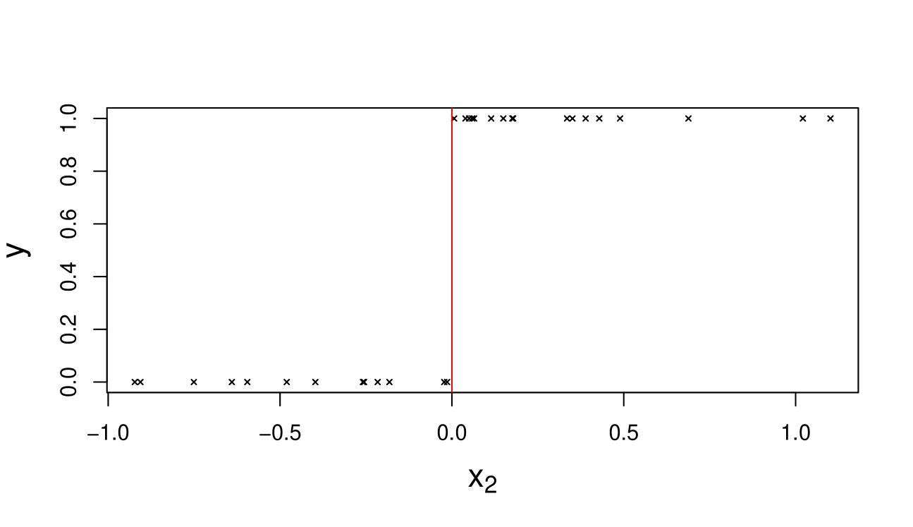
First, we generate a dataset with (including the intercept) and . The continuous predictor is chosen to be a solitary separator (after standardizing), which leads to complete separation, whereas the constant term contains all one’s and is not a solitary separator. A plot of versus in Figure 2 demonstrates this graphically. So by Theorem 1, under independent Cauchy priors, exists but does not.
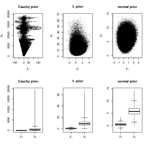
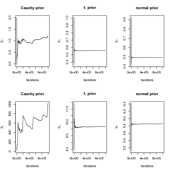
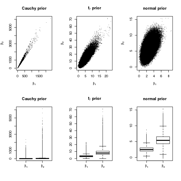
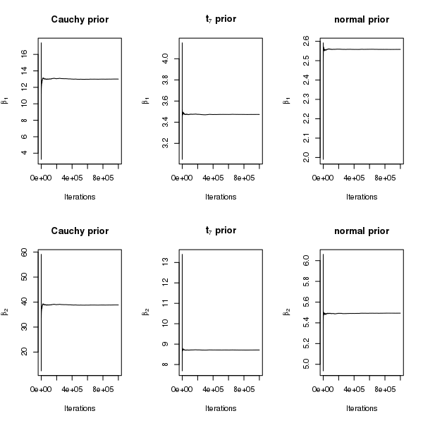
The results from the Gibbs sampler are reported in Figures 3 and 4. Figure 3 shows the posterior samples of under the different priors. The scale of , the coefficient corresponding to the solitary separator , is extremely large under Cauchy priors, less so under priors, and the smallest under normal priors. In particular, under Cauchy priors, the posterior distribution of seems to have an extremely long right tail. Moreover, although is not a solitary separator, under Cauchy priors, the posterior samples of have a much larger spread. Figure 4 shows that the running means of both and converge rapidly under normal and priors, whereas under Cauchy priors, the running mean of does not converge after a million iterations and that of clearly diverges. We also ran Stan for this example but do not report the results here, because it gave warning messages about divergent transitions for Cauchy priors, after the burn-in period. Given that the posterior mean of does not exist in this case, the lack of convergence is not surprising.
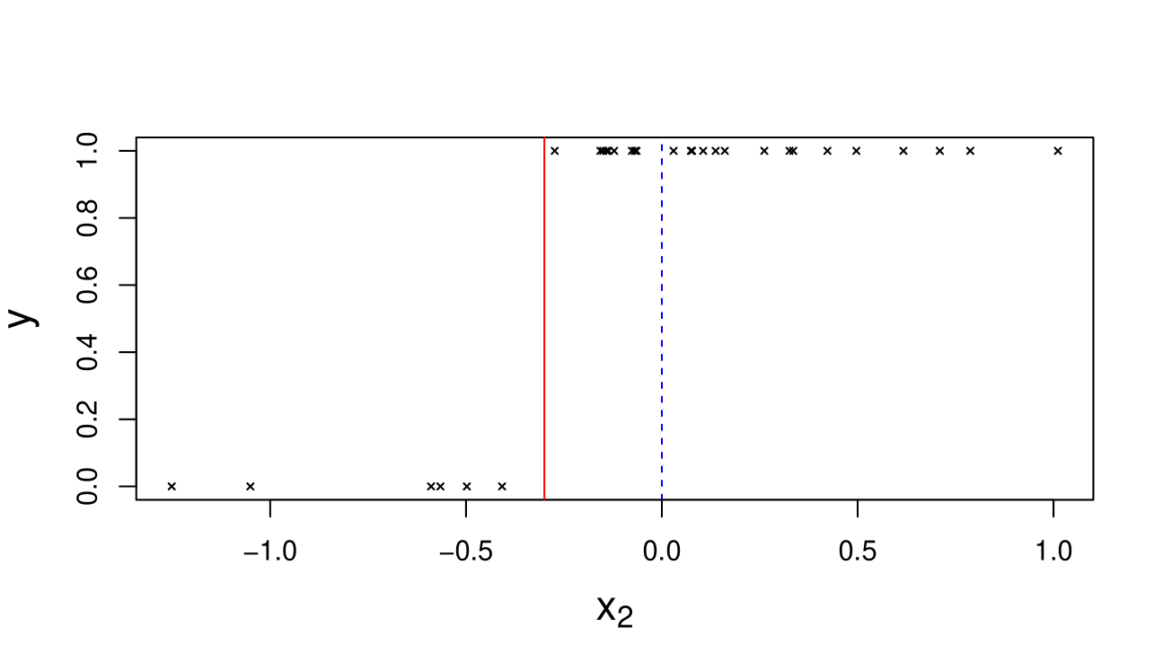
4.2 Complete Separation Without Solitary Separators
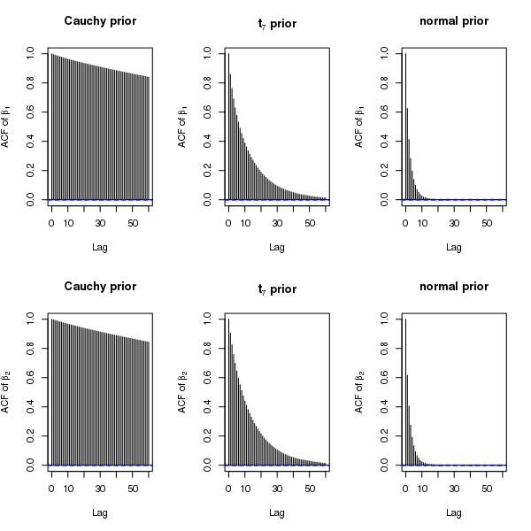
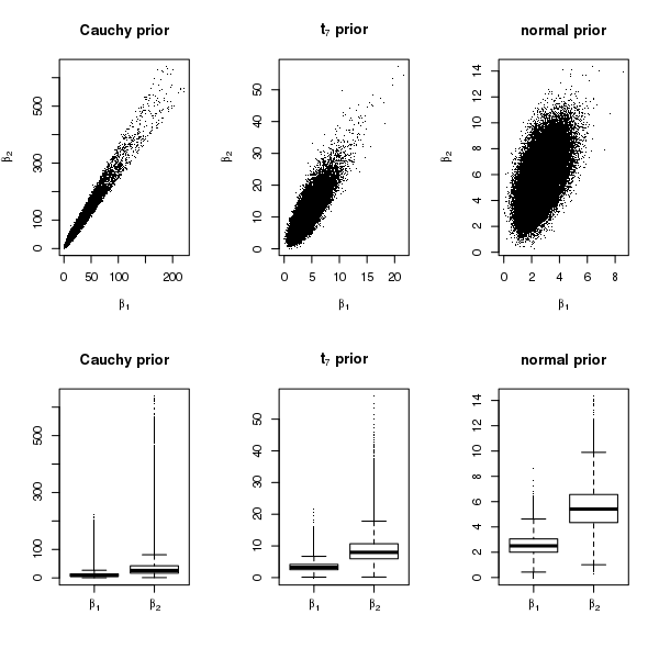
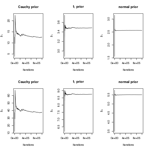
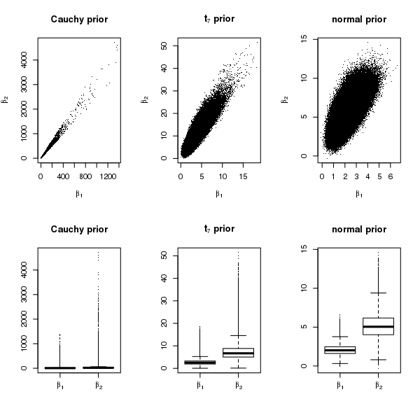
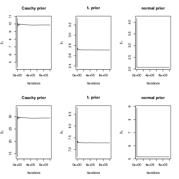
Now we generate a new dataset with and such that there is complete separation but there are no solitary separators (see Figure 5). This guarantees the existence of both and under independent Cauchy priors. The difference in the existence of for the two simulated datasets is reflected by the posterior samples from the Gibbs sampler: under Cauchy priors, the samples of in Figure 1 in the Appendix are more stabilized than those in Figure 3 in the manuscript. However, when comparing across prior distributions, we find that the posterior samples of neither nor are as stable as those under and normal priors, which is not surprising because among the three priors, Cauchy priors have the heaviest tails and thus yield the least shrinkage. Figure 2 in the Appendix shows that the convergence of the running means under Cauchy priors is slow. Although we have not verified the existence of the second or higher order posterior moments under Cauchy priors, for exploratory purposes we examine sample autocorrelation plots of the draws from the Gibbs sampler. Figure 6 shows that the autocorrelation decays extremely slowly for Cauchy priors, reasonably fast for priors, and rapidly for normal priors.
Some results from Stan are reported in Figures 3 and 4 in the Appendix. Figure 3 in the Appendix shows posterior distributions with nearly identical shapes as those obtained using Gibbs sampling in Figure 1 in the Appendix, with the only difference being that more extreme values appear under Stan. This is most likely due to faster mixing in Stan. As Stan traverses the parameter space more rapidly, values in the tails appear more quickly than under the Gibbs sampler. Figures 2 and 4 in the Appendix demonstrate that running means based on Stan are in good agreement with those based on the Gibbs sampler.
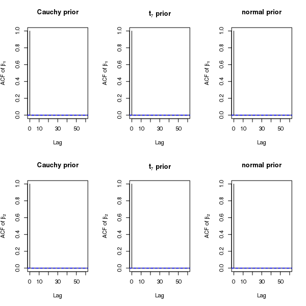
The autocorrelation plots for Stan in Figure 7 demonstrate a remarkable improvement over those for Gibbs in Figure 6 for all priors, and the difference in mixing is the most prominent for Cauchy priors.
To summarize, all the plots unequivocally suggest that Cauchy priors lead to an extremely slow mixing Gibbs sampler and unusually large scales for the regression coefficients, even when all the marginal posterior means are guaranteed to exist. While mixing can be improved tremendously with Stan, the heavy tailed posteriors under Stan are in agreement with those obtained from the Gibbs samplers. One may argue that in spite of the unnaturally large regression coefficients, Cauchy priors could lead to superior predictions. Thus in the next two sections we compare predictions based on posteriors under the three priors for two real datasets. As Stan generates nearly independent samples, we use Stan for MCMC simulations for the real datasets.
5 Real Data
5.1 SPECT Dataset
The “SPECT” dataset (Kurgan et al. 2001) is available from the UCI Machine Learning Repository111https://archive.ics.uci.edu/ml/datasets/SPECT+Heart. The binary response variable is whether a patient’s cardiac image is normal or abnormal, according to the diagnosis of cardiologists. The predictors are 22 binary features obtained from the cardiac images using a machine learning algorithm. The goal of the study is to determine if the predictors can correctly predict the diagnoses of cardiologists, so that the process could be automated to some extent.
Prior to centering, two of the binary predictors are solitary quasicomplete separators: and , for , with denoting the column of ones. Ghosh and Reiter (2013) analyzed this dataset with a Bayesian probit regression model which incorporated variable selection. As some of their proposed methods relied on an approximation of the marginal likelihood based on the MLE of , they had to drop these potentially important predictors from the analysis. If one analyzed the dataset with the uncentered predictors, by Theorem 1, the posterior means and would not exist under independent Cauchy priors. However, after centering there are no solitary separators, so the posterior means of all coefficients exist.
The SPECT dataset is split into a training set of 80 observations and a test set of 187 observations by Kurgan et al. (2001). We use the former for model fitting and the latter for prediction. First, for each of the three priors (Cauchy, , and normal), we run Stan on the training dataset, for 1,000,000 iterations after discarding 100,000 samples as burn-in.
As in the simulation study, MCMC draws from Stan show excellent mixing for all priors. However, the posterior means of the regression coefficients involved in separation are rather large under Cauchy priors compared to the other priors. For example, the posterior means of under Cauchy, , and normal priors are and respectively. These results suggest that Cauchy priors are too diffuse for datasets with separation.
Next for each in the test set, we estimate the corresponding success probability by the Monte Carlo average:
| (11) |
where is the sampled value of in iteration , after burn-in. Recall that here and . We calculate two different types of summary measures to assess predictive performance. We classify the th observation in the test set as a success, if and as a failure otherwise, and compute the misclassification rates. Note that the misclassification rate does not fully take into account the magnitude of . For example, if both and would correctly classify the observation, while the latter may be more preferable. So we also consider the average squared difference between and :
| (12) |
which is always between 0 and 1, with a value closer to 0 being more preferable. Note that the Brier score (Brier 1950) equals , according to its original definition. Since in some modified definitions (Blattenberger and Lad 1985), it is the same as , we refer to as the Brier score.
| Cauchy | normal | ||
|---|---|---|---|
| MCMC | 0.273 | 0.257 | 0.251 |
| EM | 0.278 | 0.262 | 0.262 |
| Cauchy | normal | ||
|---|---|---|---|
| MCMC | 0.172 | 0.165 | 0.163 |
| EM | 0.179 | 0.178 | 0.178 |
To compare the Monte Carlo estimates with those based on the EM algorithm of Gelman et al. (2008), we also estimate the posterior mode, denoted by under identical priors and hyperparameters, using the R package arm (Gelman et al. 2015). The EM estimator of is given by:
| (13) |
and is calculated by replacing by in (12).
We report the misclassification rates in Table 1 and the Brier scores in Table 2. MCMC achieves somewhat smaller misclassification rates and Brier scores than EM, especially under and normal priors. This suggests that a full Bayesian analysis using MCMC may produce estimates that are closer to the truth than modal estimates based on the EM algorithm. The predictions are similar across the three prior distributions with the normal and priors yielding slightly more accurate results than Cauchy priors.
5.2 Pima Indians Diabetes Dataset
We now analyze the “Pima Indians Diabetes” dataset in the R package MASS. This is a classic dataset without separation that has been analyzed by many authors in the past. Using this dataset we aim to compare predictions under different priors, when there is no separation. Using the training data provided in the package we predict the class labels of the test data. In this case the difference between different priors is practically nil. The Brier scores are same up to three decimal places, across all priors and all methods (EM and MCMC). The misclassification rates reported in Table 3 also show negligible difference between priors and methods. Here Cauchy priors have a slightly better misclassification rate compared to normal and priors, and MCMC provides slightly more accurate results compared to those obtained from EM. These results suggest that when there is no separation and maximum likelihood estimates exist, Cauchy priors may be preferable as default weakly informative priors in the absence of real prior information.
| Cauchy | normal | ||
|---|---|---|---|
| MCMC | 0.196 | 0.199 | 0.199 |
| EM | 0.202 | 0.202 | 0.202 |
6 Discussion
We have proved that posterior means of regression coefficients in logistic regression are not always guaranteed to exist under the independent Cauchy priors recommended by Gelman et al. (2008), if there is complete or quasicomplete separation in the data. In particular, we have introduced the notion of a solitary separator, which is a predictor capable of separating the samples on its own. Note that a solitary separator needs to be able to separate without the aid of any other predictor, not even the constant term corresponding to the intercept. We have proved that for independent Cauchy priors, the absence of solitary separators is a necessary condition for the existence of posterior means of all coefficients, for a general family of link functions in binary regression models. For logistic and probit regression, this has been shown to be a sufficient condition as well. In general, the sufficient condition depends on the form of the link function. We have also studied multivariate Cauchy priors, where the solitary separator no longer plays an important role. Instead, posterior means of all predictors exist if there is no separation, while none of them exist if there is complete separation. The result under quasicompelte separation is still unclear and will be studied in future work.
In practice, after centering the input variables it is straightforward to check if there are solitary separators in the dataset. The absence of solitary separators guarantees the existence of posterior means of all regression coefficients in logistic regression under independent Cauchy priors. However, our empirical results have shown that even when the posterior means for Cauchy priors exist under separation, the posterior samples of the regression coefficients may be extremely large in magnitude. Separation is usually considered to be a sample phenomenon, so even if the predictors involved in separation are potentially important, some shrinkage of their coefficients is desirable through the prior. Our empirical results based on real datasets have demonstrated that the default Cauchy priors can lead to posterior means as large as 10, which is considered to be unusually large on the logit scale. Our impression is that Cauchy priors are good default choices in general because they contain weak prior information and let the data speak. However, under separation, when there is little information in the data about the logistic regression coefficients (the MLE is not finite), it seems that lighter tailed priors, such as Student- priors with larger degrees of freedom or even normal priors, are more desirable in terms of producing more plausible posterior distributions.
From a computational perspective, we have observed very slow convergence of the Gibbs sampler under Cauchy priors in the presence of separation. Note that if the design matrix is not of full column rank, for example when , the columns of will be linearly dependent. This implies that the equation for quasicomplete separation (3) will be satisfied with equality for all observations. Empirical results (not reported here for brevity) demonstrated that independent Cauchy priors show convergence of the Gibbs sampler in this case also compared to other lighter tailed priors. Out-of-sample predictive performance based on a real dataset with separation did not show the default Cauchy priors to be superior to or normal priors.
In logistic regression, under a multivariate normal prior for , Choi and Hobert (2013) showed that the Pólya-Gamma data augmentation Gibbs sampler of Polson et al. (2013) is uniformly ergodic, and the moment generating function of the posterior distribution exists for all . In our examples of datasets with separation, the normal priors led to the fastest convergence of the Gibbs sampler, reasonable scales for the posterior draws of , and comparable or even better predictive performance than other priors. The results from Stan show no problem in mixing under any of the priors. However, the problematic issue of posteriors with extremely heavy tails under Cauchy priors cannot be resolved without altering the prior. Thus, after taking into account all the above considerations, for a full Bayesian analysis we recommend the use of normal priors as a default, when there is separation. Alternatively, heavier tailed priors such as the could also be used if robustness is a concern. On the other hand, if the goal of the analysis is to obtain point estimates rather than the entire posterior distribution, the posterior mode obtained from the EM algorithm of Gelman et al. (2015) under default Cauchy priors (Gelman et al. 2008) is a fast viable alternative.
Supplementary Material
In the supplementary material, we present additional simulation results for logistic and probit regression with complete separation, along with an appendix that contains the proofs of all theoretical results. The Gibbs sampler developed in the paper can be implemented with the R package tglm, available from the website: https://cran.r-project.org/web/packages/tglm/index.html.
Acknowledgement
The authors thank the Editor-in-Chief, Editor, Associate Editor and the reviewer for suggestions that led to a greatly improved paper. The authors also thank Drs. David Banks, James Berger, William Bridges, Merlise Clyde, Jon Forster, Jayanta Ghosh, Aixin Tan, and Shouqiang Wang for helpful discussions. The research of Joyee Ghosh was partially supported by the NSA Young Investigator grant H98230-14-1-0126.
Supplementary Material: On the Use of Cauchy Prior Distributions for Bayesian Logistic Regression
In this supplement, we first present an appendix with additional simulation results for logit and probit link functions, and then include an appendix that contains proofs of the theoretical results.
1 Appendix: Simulation Results for Complete Separation Without Solitary Separators
In this section we present some supporting figures for the analysis of the simulated dataset described in Section 4.2 of the manuscript under logit and probit links.
1.1 Logistic Regression for Complete Separation Without Solitary Separators
Figures 1 and 2 are based on the posterior samples from a Gibbs sampler under a logit link, whereas Figures 3 and 4 are corresponding results from Stan. A detailed discussion of the results is provided in Section 4.2 of the manuscript.
1.2 Probit Regression for Complete Separation Without Solitary Separators
In this section we analyze the simulated dataset described in Section 4.2 of the manuscript under a probit link, while keeping everything else the same. We have shown in Theorem 2, that the theoretical results hold for a probit link. The goal of this analysis is to demonstrate that the empirical results are similar under the logit and probit link functions. For this dataset, Theorem 2 guarantees the existence of both and under independent Cauchy priors and a probit link function. As in the case of logistic regression the heavy tails of Cauchy priors translate into an extremely heavy right tail in the posterior distributions of and , compared to the lighter tailed priors (see Figure 5 and 6 here). Thus in the case of separation, normal priors seem to be reasonable for probit regression also.
2 Appendix: Proofs
First, we decompose the proof of Theorem 1 into two parts: in Appendix A we show that a necessary condition for the existence of is that is not a solitary separator; and in Appendix B we show that it is also a sufficient condition. Then, we prove Theorem 2 in Appendix C, and Corollary 1 in Appendix D. Finally, we decompose the proof of Theorem 3 into two parts: in Appendix E we show that all posterior means exist if there is no separation; then in Appendix F we show that none of the posterior means exist if there is complete separation.
A Proof of the Necessary Condition for Theorem 1
Here we show that if is a solitary separator, then does not exist, which is equivalent to the necessary condition for Theorem 1.
Proof.
For notational simplicity, we define the functional form of the success and failure probabilities in logistic regression as
| (A.1) |
which are strictly increasing and decreasing functions of , respectively. In addition, both functions are bounded: for . Let and denote the vectors and after excluding their th entries and , respectively. Then the likelihood function can be written as
| (A.2) |
The posterior mean of exists provided . When the posterior mean exists it is given by (4). Clearly if one of the two integrals in (4) is not finite, then . In this proof we will show that if , the first integral in (4) equals . Similarly, it can be shown that if , the second integral in (4) equals .
If , by (2)-(5), for all , and for all . When , by the monotonic property of and we have, , which is free of . Therefore,
| (A.3) |
Here the first equation results from independent priors, i.e., . Since , . Moreover, for all , so we also have , implying that . For the independent Cauchy priors in (6), and the second integral in (A.3) is positive, hence (A.3) equals . ∎
B Proof of the Sufficient Condition for Theorem 1
Here we show that if is not a solitary separator, then the posterior mean of exists.
Proof.
When the posterior mean of exists and is given by
| (B.1) |
Since it is enough to show that the positive term has a finite upper bound, and the negative term has a finite lower bound. For notational simplicity, in the remainder of the proof, we let , , , and denote the vectors , , , and after excluding their th entries, respectively.
We first show that has a finite upper bound. Because is not a solitary separator, there exists either
-
(a)
an such that , or
-
(b)
a , such that .
If both (a) and (b) are violated then is a solitary separator and leads to a contradiction. Furthermore, for such or , it contains at least one non-zero entry. This is because if , i.e., does not correspond to the intercept (the column of all one’s), then the first entry in or equals . If , due to the assumption that has a column rank , there exists one row such that contains at least one non-zero entry. If , then we let and the condition (b) holds because . If , we may first rescale by , which transforms to . Since the Cauchy prior centered at zero is invariant to this rescaling, and exists if and only if exists, we can just apply this rescaling, after which . Then we let and the condition (a) holds.
We first assume that condition (a) is true. We define a positive constant . For any , we define a subset of the domain of as follows
| (B.2) |
Then for any , . Therefore,
| (B.3) |
As and are bounded above by 1, the likelihood function in (A.2) is bounded above by . Thus
| (B.4) |
Here the last inequality results from (B.3) and the fact that the function is bounded above by . An upper bound is obtained for the first term in the bracket in (B.4) using the fact that the integrand is non-negative as follows:
| (B.5) |
Recall that contains at least one non-zero entry. We assume that . Then to simplify the second term in the bracket in (B.4), we transform to via a linear transformation, such that , and is the vector after excluding . The characteristic function of a Cauchy distribution is , where . Since a priori, is a linear combination of independent random variables, , for , its characteristic function is
So the induced prior of is . Let denote the vector obtained by taking absolute values of each element of , then the above scale parameter = . By (B.2), for any , the corresponding and . An upper bound is calculated for the second term in the bracket in (B.4). Note that is the joint density of and . Since it incorporates the Jacobian of transformation from to and , a separate Jacobian term is not needed in the first equality below.
| (B.6) |
Here, the second equality holds because ; the last inequality holds because and are both positive, and for any , .
Then substituting the expression for as in (6), we continue with (B.4) to find an upper bound.
| (B.7) |
On the other hand, if condition (b) holds, then we just need to slightly modify the above proof. We define , and change (B.2) to
Consequently, the terms and in (B.4) have to be changed to and , respectively. For the logit link, . The range of the integral in (B.6) with respect to is from to ; however, because the density of is symmetric around 0, the value of the integral stays the same. So it can be shown an upper bound for is .
We now show that the negative term has a finite lower bound. For any , by expressing , we need to show that the positive term has a finite upper bound. As the idea is very similar to the proof of existence of , we present less details here.
Since the predictor is not a solitary separator, there exists either
-
(c)
an such that , or
-
(d)
a , such that .
If (c) and (d) are both violated has to be a solitary separator, which leads to a contradiction. WLOG, we assume that condition (c) is true, and as before must contain at least one non-zero entry, say, . If condition (d) is true, then we can adopt a modification similar to the one that is used to prove the existence under condition (b) based on the proof under condition (a).
We define a positive constant . For any , we define a subset of as . Then for all , , hence . Since the likelihood function ,
| (B.8) |
The first term in the bracket in (B.8) has an upper bound as in (B.5). Recall that . We now transform to via a linear transformation, such that and is the vector after excluding . The prior of is . For any , the corresponding . Therefore as in (B.6), we obtain an upper bound for the second term in the bracket in (B.8) as . Finally, following (B.7) an upper bound for is . ∎
C Proof of Theorem 2
Proof.
Following the proof of Theorem 1, we denote the success probability function by , where is the inverse link function, i.e., . Similarly, let the failure probability function be . Note that the proof of the necessary condition for Theorem 1 given in Appendix A only relies on the fact the is increasing, continuous, and bounded between and . Since the link function is assumed to be strictly increasing and differentiable, so is . Moreover, the range of is . Therefore, the proof of the necessary condition for Theorem 2 follows immediately.
For the proof of the sufficient condition in Theorem 2, one can follow the proof in Appendix B and proceed with the specific choice of used there, when condition (a) holds. The proof is identical until (B.4) because the explicit form of the inverse link function is not used until that step. We re-write the final step in (B.4) below and proceed from there:
| (C.1) |
The sufficient condition in Theorem 2 states that for every positive constant ,
This implies that the integral will be bounded for the specific choice of used in the above proof, and hence the first integral in (C.1) is bounded above. The second integral does not depend on the link function and its bound can be obtained exactly as in Appendix B. Thus under condition (a). On the other hand if condition (b) holds, the proof follows similarly as in Appendix B and now we need to use the sufficient condition in Theorem 2 that for every positive constant , . A bound for can be obtained similarly, which completes the proof.
In probit regression, we first show that
| (C.2) |
where is the standard normal cdf. It is equivalent to show that the difference function
| (C.3) |
Note that , and . Since is differentiable, we have
Now , and when is very small, since decays to zero at a faster speed than , i.e., there exists a such that . Since is a continuous function, the intermediate value theorem applied to shows that there exists a such that . Therefore, to show (C.3), it is sufficient to show that has a unique root on , which is proved by contradiction as follows.
If has two distinct roots , i.e., for , , then
| (C.4) |
Note that the derivative of the function is . It is straightforward to show that this derivative is strictly less than 0 for all , so is a strictly decreasing function. Thus (C.4) holds only if , which leads to a contradiction.
Hence for any ,
Since the probit link is symmetric, i.e., , we also have . ∎
D Proof of Corollary 1
To prove Corollary 1, we mainly use a similar strategy to the proof of Theorem 1. To show the necessary condition, we can use all of Appendix A without modification, for both logistic and probit regression models. To show the sufficient condition, we can follow the same proof outline as in Appendix B, with some minimal modification as described in the following proof.
Proof.
First, we denote the vector of prior location parameters by . If we shift the coefficients by units, then
that is, the resulting parameters have independent Cauchy priors with location parameters being zero. Since the original parameter for each , the existence of is equivalent to the existence of . So we just need to show that if is not a solitary separator, then exists. For simplicity, here we just show that the positive term
has a finite upper bound. The other half of the result that the negative term has a finite lower bound will follow with a similar derivation.
As in Appendix B, we first assume that condition (a) is true, and define in the same way. For any , we define a subset of the domain of as follows
then for any , . Since is an increasing function,
A similar derivation to (B.4) gives
where by (B.5) the first integral inside the bracket has an upper bound
| (D.1) |
and by (B.6) the second integral inside the bracket also has an upper bound
In probit regression, the function in the above derivations equals the standard normal cdf . By (C.2), for any , we have
Hence for we have an upper bound
Note that a similar derivation also holds if .
E Proof of Theorem 3, in the case of no separation
Proof.
For any , to show that exists, we just need to show the positive term in (B.1) has an upper bound, because the negative term in (B.1) having a lower bound follows a similar derivation.
When working on , we only need to consider positive . Denote a new dimensional variable , then for ,
If there is no separation, for any , there exists at least one , such that
| (E.1) |
For each , denote the vector and the function as follows,
| (E.2) |
then (E.1) can be rewritten as . Denote for ,
Then each is a non-empty subset of , unless and . Let denote the set of indices , for which the corresponding are non-empty. Because there is no separation,
| (E.3) |
Hence, the set is non-empty. We denote its size by , and rewrite .
Now we show that there exist positive constants , such that
| (E.4) |
where
| (E.5) |
are subsets of the corresponding , for all .
If there exists an such that and , then . In this case, we just need to let , and , for all , where is an arbitrary positive number. Under this choice of ’s, the sets ’s defined by (E.5) satisfy (E.4).
If, on the other hand, for all , i.e., all are open half spaces in , then we can find the constants sequentially. For , if , we can set . Then the resulting defined by (E.5) satisfies
| (E.6) |
If , then (E.3) suggests
| (E.7) |
For (E.6) to hold, we just need to find an positive such that the resulting has as a subset, i.e., should be larger than the maximum of over the polyhedral region . Note that maximizing over the polyhedron can be represented as a linear programming question,
| maximize | (E.8) | |||
| subject to | ||||
By Bertsimas and Tsitsiklis (1997, pp. 67, Corollary 2.3), for any linear programming problem over a non-empty polyhedron, including the one in (E.8) to maximize , either the optimal , or there exists an optimal solution, . Here, the latter case always occurs, because by (E.7), the maximum of over the polyhedron does not exceed zero, so it does not go to infinity. Hence, we just need to let
so that the resulting contains as a subset, which yields (E.6). After finding , we can apply similar procedures sequentially, to find positive values , for , such that
After identifying all ’s, the resulting ’s satisfy (E.4). Note that the choice of ’s only depend on the data , , so they are constants given the observed data.
For each , next we show that for any , the likelihood function of the th observation is bounded above by . This is because in a logistic regression, if , then
| (E.9) |
if , then
| (E.10) |
Here, the last inequality holds because for any . By (C.2), in a probit regression model, the inequalities (E.9) and (E.10) also hold.
Now we show that the positive term has a finite upper bound.
∎
Note that in Appendix E, the specific formula of the prior density of is not used. Therefore, if there is no separation in logistic or probit regression, posterior means of all coefficients exist under all proper prior distributions.
F Proof of Theorem 3, in the case of complete separation
Proof.
Here we show that if there is complete separation, then none of the posterior means exist, for . Using the notation , defined in (E.2), we rewrite the set of all vectors satisfying the complete separation condition (2) as
According to Albert and Anderson (1984), is a convex cone; moreover, if , then for any that is small enough. Hence, the open set , as a subset of the Euclidean space, has positive Lebesgue measure.
To show that does not exist, if projects on the positive half of the axis, we will show that diverges, otherwise, we will show that diverges (if both, then showing either is sufficient). Now we assume that the former is true, and denote the intersection
which is again an open convex cone. Since has positive measure in , under the change of variable from to , where , there exists an open set such that can be written as
Suppose that can be written as . We define a variant of it by , such that . Under the multivariate Cauchy prior (8), the induced prior distribution of is
Inside , there must exist a closed rectangular box, denoted by . By Browder (1996, pp. 142, Corollary 6.57), a continuous function takes its maximum and minimum on a compact set. Since is a compact set (closed and bounded in ),
| (F.1) |
both exist.
Recall that for all (hence including all elements in ), ; equivalently, if , then , and if , then . Now we show that in both logistic and probit regressions, the positive term diverges.
| (F.2) | ||||
where is a positive constant, is a constant, and and have been defined previously in (F.1).
On the other hand, if the set of complete separation vectors only projects on the negative half of the axis, following a similar deviation, we can show that diverges to .
∎
References
- Albert and Anderson (1984) Albert, A. and Anderson, J. A. (1984). “On the Existence of Maximum Likelihood Estimates in Logistic Regression Models.” Biometrika, 71(1): 1–10.
- Bardenet et al. (2014) Bardenet, R., Doucet, A., and Holmes, C. (2014). “Towards Scaling up Markov Chain Monte Carlo: An Adaptive Subsampling Approach.” Proceedings of the 31st International Conference on Machine Learning (ICML-14), 405–413.
- Bertsimas and Tsitsiklis (1997) Bertsimas, D. and Tsitsiklis, J. N. (1997). Introduction to Linear Optimization. Athena Scientific Belmont, MA.
- Bickel and Doksum (2001) Bickel, P. J. and Doksum, K. A. (2001). Mathematical Statistics, volume I. Prentice Hall Englewood Cliffs, NJ.
- Blattenberger and Lad (1985) Blattenberger, G. and Lad, F. (1985). “Separating the Brier Score into Calibration and Refinement Components: A Graphical Exposition.” The American Statistician, 39(1): 26–32.
- Brier (1950) Brier, G. W. (1950). “Verification of Forecasts Expressed in Terms of Probability.” Monthly Weather Review, 78: 1–3.
- Browder (1996) Browder, A. (1996). Mathematical Analysis: An Introduction. Springer-Verlag.
- Carpenter et al. (2016) Carpenter, B., Gelman, A., Hoffman, M., Lee, D., Goodrich, B., Betancourt, M., Brubaker, A., Michael, Guo, J., Li, P., and Riddell, A. (2016). “Stan: A Probabilistic Programming Language.” Journal of Statistical Software, in press.
- Casella and Berger (1990) Casella, G. and Berger, R. L. (1990). Statistical Inference. Duxbury Press.
- Chen and Shao (2001) Chen, M.-H. and Shao, Q.-M. (2001). “Propriety of Posterior Distribution for Dichotomous Quantal Response Models.” Proceedings of the American Mathematical Society, 129(1): 293–302.
- Choi and Hobert (2013) Choi, H. M. and Hobert, J. P. (2013). “The Polya-Gamma Gibbs Sampler for Bayesian Logistic Regression is Uniformly Ergodic.” Electronic Journal of Statistics, 7(2054-2064).
- Chopin and Ridgway (2015) Chopin, N. and Ridgway, J. (2015). “Leave Pima Indians Alone: Binary Regression as a Benchmark for Bayesian Computation.” arxiv.org.
- Clogg et al. (1991) Clogg, C. C., Rubin, D. B., Schenker, N., Schultz, B., and Weidman, L. (1991). “Multiple Imputation of Industry and Occupation Codes in Census Public-Use Samples Using Bayesian Logistic Regression.” Journal of the American Statistical Association, 86(413): 68–78.
- Dawid (1973) Dawid, A. P. (1973). “Posterior Expectations for Large Observations.” Biometrika, 60: 664–666.
- Fernández and Steel (2000) Fernández, C. and Steel, M. F. (2000). “Bayesian Regression Analysis with Scale Mixtures of Normals.” Econometric Theory, 16(80-101).
- Firth (1993) Firth, D. (1993). “Bias Reduction of Maximum Likelihood Estimates.” Biometrika, 80(1): 27–38.
- Fouskakis et al. (2009) Fouskakis, D., Ntzoufras, I., and Draper, D. (2009). “Bayesian Variable Selection Using Cost-Adjusted BIC, with Application to Cost-Effective Measurement of Quality of Health Care.” The Annals of Applied Statistics, 3(2): 663–690.
- Gelman et al. (2008) Gelman, A., Jakulin, A., Pittau, M., and Su, Y. (2008). “A Weakly Informative Default Prior Distribution for Logistic and Other Regression Models.” The Annals of Applied Statistics, 2(4): 1360–1383.
-
Gelman et al. (2015)
Gelman, A., Su, Y.-S., Yajima, M., Hill, J., Pittau, M. G., Kerman, J., Zheng,
T., and Dorie, V. (2015).
arm: Data Analysis Using Regression and Multilevel/Hierarchical
Models.
R package version 1.8-5.
URL http://CRAN.R-project.org/package=arm - Ghosh and Clyde (2011) Ghosh, J. and Clyde, M. A. (2011). “Rao-Blackwellization for Bayesian Variable Selection and Model Averaging in Linear and Binary Regression: A Novel Data Augmentation Approach.” Journal of the American Statistical Association, 106(495): 1041–1052.
- Ghosh et al. (2011) Ghosh, J., Herring, A. H., and Siega-Riz, A. M. (2011). “Bayesian Variable Selection for Latent Class Models.” Biometrics, 67: 917–925.
- Ghosh and Reiter (2013) Ghosh, J. and Reiter, J. P. (2013). “Secure Bayesian Model Averaging for Horizontally Partitioned Data.” Statistics and Computing, 23: 311–322.
- Gramacy and Polson (2012) Gramacy, R. B. and Polson, N. G. (2012). “Simulation-Based Regularized Logistic Regression.” Bayesian Analysis, 7(3): 567–590.
- Hanson et al. (2014) Hanson, T. E., Branscum, A. J., and Johnson, W. O. (2014). “Informative g-Priors for Logistic Regression.” Bayesian Analysis, 9(3): 597–612.
- Heinze (2006) Heinze, G. (2006). “A Comparative Investigation of Methods for Logistic Regression with Separated or Nearly Separated Data.” Statistics in Medicine, 25: 4216–4226.
- Heinze and Schemper (2002) Heinze, G. and Schemper, M. (2002). “A Solution to the Problem of Separation in Logistic Regression.” Statistics in Medicine, 21: 2409–2419.
- Hoffman and Gelman (2014) Hoffman, M. D. and Gelman, A. (2014). “The No-U-Turn Sampler: Adaptively Setting Path Lengths in Hamiltonian Monte Carlo.” The Journal of Machine Learning Research, 15(1): 1593–1623.
- Holmes and Held (2006) Holmes, C. C. and Held, L. (2006). “Bayesian Auxiliary Variable Models for Binary and Multinomial Regression.” Bayesian Analysis, 1(1): 145–168.
- Ibrahim and Laud (1991) Ibrahim, J. G. and Laud, P. W. (1991). “On Bayesian Analysis of Generalized Linear Models using Jeffreys’s Prior.” Journal of the American Statistical Association, 86(416): 981–986.
- Jeffreys (1961) Jeffreys, H. (1961). Theory of Probability. Oxford Univ. Press.
- Kurgan et al. (2001) Kurgan, L., Cios, K., Tadeusiewicz, R., Ogiela, M., and Goodenday, L. (2001). “Knowledge Discovery Approach to Automated Cardiac SPECT Diagnosis.” Artificial Intelligence in Medicine, 23:2: 149–169.
- Li and Clyde (2015) Li, Y. and Clyde, M. A. (2015). “Mixtures of -Priors in Generalized Linear Models.” arxiv.org.
- Liu (2004) Liu, C. (2004). “Robit Regression: A Simple Robust Alternative to Logistic and Probit Regression.” In Gelman, A. and Meng, X. (eds.), Applied Bayesian Modeling and Casual Inference from Incomplete-Data Perspectives, 227–238. Wiley, London.
- McCullagh and Nelder (1989) McCullagh, P. and Nelder, J. (1989). Generalized Linear Models. Chapman and Hall.
- Mitra and Dunson (2010) Mitra, R. and Dunson, D. B. (2010). “Two Level Stochastic Search Variable Selection in GLMs with Missing Predictors.” International Journal of Biostatistics, 6(1): Article 33.
- Neal (2003) Neal, R. M. (2003). “Slice Samlping.” The Annals of Statistics, 31(3): 705–767.
- Neal (2011) — (2011). “MCMC using Hamiltonian Dynamics.” In Brooks, S., Gelman, A., Jones, G., and Meng, X.-L. (eds.), Handbook of Markov Chain Monte Carlo. Chapman & Hall / CRC Press.
- O’Brien and Dunson (2004) O’Brien, S. M. and Dunson, D. B. (2004). “Bayesian Multivariate Logistic Regression.” Biometrics, 60(3): 739–746.
- Polson et al. (2013) Polson, N. G., Scott, J. G., and Windle, J. (2013). “Bayesian Inference for Logistic Models Using Pólya-Gamma Latent Variables.” Journal of the American Statistical Association, 108(504): 1339–1349.
- Rousseeuw and Christmann (2003) Rousseeuw, P. J. and Christmann, A. (2003). “Robustness Against Separation and Outliers in Logistic Regression.” Computational Statistics and Data Analysis, 42: 315–332.
- Sabanés Bové and Held (2011) Sabanés Bové, D. and Held, L. (2011). “Hyper- Priors for Generalized Linear Models.” Bayesian Analysis, 6(3): 387–410.
- Speckman et al. (2009) Speckman, P. L., Lee, J., and Sun, D. (2009). “Existence of the MLE and Propriety of Posteriors for a General Multinomial Choice Model.” Statistica Sinica, 19: 731–748.
- Yang and Berger (1996) Yang, R. and Berger, J. O. (1996). “A Catalog of Noninformative Priors.” Institute of Statistics and Decision Sciences, Duke University.
- Zellner and Siow (1980) Zellner, A. and Siow, A. (1980). “Posterior Odds Ratios for Selected Regression Hypotheses.” In Bayesian Statistics: Proceedings of the First International Meeting Held in Valencia (Spain), 585–603. Valencia, Spain: University of Valencia Press.
- Zorn (2005) Zorn, C. (2005). “A Solution to Separation in Binary Response Models.” Political Analysis, 13(2): 157–170.