One-dimensional radiation-hydrodynamic simulations of imploding spherical plasma liners with detailed equation-of-state modeling
Abstract
This work extends the one-dimensional radiation-hydrodynamic imploding spherical argon plasma liner simulations of T. J. Awe et al. [Phys. Plasmas 18, 072705 (2011)] by using a detailed tabular equation-of-state (EOS) model, whereas Awe et al. used a polytropic EOS model. Results using the tabular EOS model give lower stagnation pressures by a factor of 3.9–8.6 and lower peak ion temperatures compared to the polytropic EOS results. Both local thermodynamic equilibrium (LTE) and non-LTE EOS models were used in this work, giving similar results on stagnation pressure. The lower stagnation pressures using a tabular EOS model are attributed to a reduction in the liner’s ability to compress arising from the energy sink introduced by ionization and electron excitation, which are not accounted for in a polytropic EOS model. Variation of the plasma liner species for the same initial liner geometry, mass density, and velocity was also explored using the LTE tabular EOS model, showing that the highest stagnation pressure is achieved with the highest atomic mass species for the constraints imposed.
I Introduction
The Plasma Liner Experiment (PLX) at Los Alamos National Laboratory was designed to form and study spherically imploding plasma liners via the merging of thirty supersonic plasma jets.Hsu et al. (2012) Such imploding plasma liners could potentially allow repetitive generation of cm-, s-, and Mbar-scale plasmas for fundamental high energy density plasma physics studies, or (if scaled up in energy) be used as a standoff compression driverThio et al. (1999, 2001); Hsu et al. (2012) for magneto-inertial fusion (MIF).Lindemuth and Kirkpatrick (1983); Kirkpatrick, Lindemuth, and Ward (1995); Lindemuth and Siemon (2009) Recent one-dimensional (1D) radiation-hydrodynamic simulations of targetless imploding spherical argon plasma liners by Awe et al.Awe et al. (2011) used a polytropic equation-of-state (EOS) model, providing insight into the 1D physical evolution of imploding spherical plasma liners, and showing that PLX-relevant plasma liner kinetic energies of hundreds of kJ could result in liner stagnation pressures on the order of 1 Mbar sustained for order 1 s. The results of Awe et al.Awe et al. (2011) indicated high enough plasma temperatures (10’s of eV) for ionization effects, which are not included in a polytropic EOS model, to have an appreciable impact on both the predicted peak pressures and temperatures. As some of the initial liner kinetic energy would now be used for ionization, it is expected that the liner may compress less, although the expected drop in thermal energy in the imploding plasma liner due to ionization and radiative loss channels are expected to help compensate. Note that this work and that of Awe et al.Awe et al. (2011) focus on targetless, self-collapse of the liner, motivated by the goals of the PLX project. Thus, care must be taken in using these results to provide insight into plasma liner implosions onto a magnetized target for MIF, which has been explored in several other recent publications.Parks (2008); Cassibry et al. (2009); Samulyak, Parks, and Wu (2010); Santarius (2012)
The purpose of this work is to develop insight into how a detailed EOS model, and particularly ionization, affect spherically symmetric, targetless plasma liner implosions. We used the HELIOS-CRMacFarlane, Golovkin, and Woodruff (2006) 1D radiation-hydrodynamic code and the PROPACEOSMacFarlane, Golovkin, and Woodruff (2006) EOS and multi-group opacity database to repeat the simulation cases presented in Awe et al.Awe et al. (2011) In particular, we examined how the detailed EOS model affected the liner stagnation pressure (defined in Sec. II.3), the stagnation time (defined in Sec. II.3), the implosion trajectory and minimum radius achieved, and scaling behavior of as a function of initial plasma liner parameters. In all cases, we used argon as did Awe et al.Awe et al. (2011) However, for a particular initial liner geometry, mass density, and velocity (corresponding to an initial energy of 375 kJ, relevant for PLX), we also ran simulations using H, D-T, 4He, 6Li, 11B, Ne, Kr, and Xe, in addition to Ar. In this work, as in Awe et al.,Awe et al. (2011) we set aside the important issues of 3D effects of the discrete merging plasma jets and 3D convergent instabilities such as Rayleigh-Taylor and others, which are addressed elsewhere,Cassibry et al. (2012) and study spherically symmetric imploding plasma liners initiated at a jet merging radius at which plasma jets are assumed to have merged.
The remainder of the paper is organized as follows. Sec. II describes our modeling approach including the choice of liner initial conditions investigated, details of the codes used, and benchmarking against the results of Awe et al.Awe et al. (2011) Section III presents the new simulation results including (1) comparison of results using local thermodynamic equilibrium (LTE) versus non-LTE EOS tables, (2) comparison of plasma liner implosions using a LTE tabular EOS versus a polytropic EOS, (3) scaling with initial liner density and velocity, and (4) different plasma species for one liner initial condition. Section IV provides a discussion and summary.
II Modeling approach
In this section we describe the simulation initial conditions, the codes used, and benchmarking of our own polytropic EOS results against the results of Awe et al.Awe et al. (2011)
II.1 Simulation initial conditions
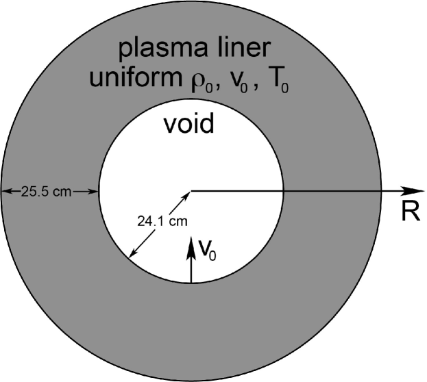
The initial conditions used in this work are shown schematically in Fig. 1 and summarized in Table 1 (columns 2–5). The rationale for these choices are described in detail in Awe et al.Awe et al. (2011) In short, they are intended to span a range of initial plasma liner velocities and kinetic energies from PLX-relevant values (50 km/s, hundreds of kJ) at the lower end to what might be needed for an MIF standoff compression driverThio et al. (1999, 2001); Hsu et al. (2012) ( km/s, tens of MJ) at the higher end. The initial liner ion density values are what can be expected based on plasma jet densities that have already been achieved by the plasma guns designed and built by HyperV TechnologiesWitherspoon et al. (2011) for use on PLX. In this work, we assume that discrete plasma jets have merged at cm and formed a spherically symmetric imploding plasma liner with uniform mass density , thickness 25.5 cm, temperature eV, and uniform inward radial velocity . The effects of non-uniform initial liner profiles are not studied here but are a potential way of optimizing imploding plasma liner performance.Kagan et al. (2011) The void region (Fig. 1) is modeled using very low density plasma with mass densities of kg/m3 (tabular EOS runs) and kg/m3 (polytropic EOS runs), temperature of 1.0 eV, and the same species as the liner. The different initial void mass densities led to slightly different computational zone setups but did not affect the overall liner evolution.
Although this work does not focus on the physical evolution of a spherical plasma liner imploding on vacuum, which was described in detail in Awe et al.,Awe et al. (2011) we provide here a brief summary of its 1D evolution: (1) the imploding liner converges toward the origin, and the liner density rises as , (2) upon the liner reaching the origin, an outward going shock propagates radially outward, shock-heating the incoming liner material, and (3) the outgoing shock reaches the outer edge of the incoming liner, at which time the high pressure of the post-shocked liner material can no longer be sustained, and the entire system disassembles.
II.2 Computational codes
This work used the HELIOS-CRMacFarlane, Golovkin, and Woodruff (2006) 1D radiation-hydrodynamic code with LTE and non-LTE EOS tables generated using the PROPACEOSMacFarlane, Golovkin, and Woodruff (2006) code. HELIOS-CR is a Lagrangian code that can use both a polytropic EOS (with adiabatic constant ) or a tabular EOS. The HELIOS-CR code has been applied previously to the modeling of inertial confinement fusion (ICF) implosions.MacFarlane et al. (2005); Welser-Sherrill et al. (2007) PROPACEOS EOS and frequency-dependent opacities are computed using a combination of an isolated atom model and, at high densities at which cohesive effects are important, a quotidian-EOS-like model.More et al. (1988) At the densities of interest in this paper, energies and pressures are computed for an isolated atom model in which atomic level populations are computed using Boltzmann statistics and the Saha equation (LTE case) or a collisional-radiative model (non-LTE case). The energies and pressures of the EOS tables are based on the free energy, thus providing for thermodynamically consistent energy and pressure values. For the non-LTE case, the effects of photoionization and photoexcitation are ignored when computing the temperature- and density- dependent tabular EOS data, as the radiation field is a non-local quantity, i.e., the radiation can originate in other parts of the plasma, and therefore is unknown when generating the tables. Detailed atomic models are utilized in which all ionization stages are included, e.g., for Ar, a total of energy levels are included. More than transitions were used for the opacity calculations. Frequency-dependent radiation transport is treated using a radiation diffusion model; fifty frequency groups were used in this work. When modeling a plasma that is not optically thick (our case) with radiation diffusion, it is possible that radiation losses could be overestimated. Finally, we checked energy conservation at s (near peak compression) for the polytropic, LTE tabular, and non-LTE tabular cases, using run 6 of Table 1 as an example. Energy is conserved to within 0.1%, 0.1%, and 1.1% for the polytropic, LTE, and non-LTE runs, respectively. These are very small effects compared to the differences we report in this paper, and thus we conclude that energy conservation does not impact our results.
We previously verifiedAwe et al. (2011) a HELIOS-CR calculation against the convergent shock Noh problemNoh (1987) and got better than 5% agreement for the highest resolution case we ran (50 m zone resolution over a sphere with 25 cm initial radius). We also did a grid resolution convergence study showing that an average grid resolution of 250 m gave % accuracy.Awe et al. (2011) In this work, we used 400 computational zones over the initially 255 mm thick liner (average of 637.5 m/zone), which was chosen based on achieving a balance between getting reasonable agreement in the benchmarking studies described in Sec. II.3 and the run time of each simulation (typically a few hours to a day per run). We used the automatic zoning feature of HELIOS-CR, and thus the zone size was much smaller than the average near boundaries and much larger elsewhere.
When using a polytropic EOS, HELIOS-CR only allows use of a one-temperature (1T) model. The tabular EOS simulations allow for separate ion and electron temperatures. All reported HELIOS-CR results with polytropic EOS are 1T, and all reported results with tabular EOS are 2T with radiation diffusion. To verify that the use of 1T versus 2T does not have a great impact on our results, we compared the time evolution of and for the zone initially at cm and saw no difference. Furthermore, the evolution from a 1T run was virtually the same as that from the 2T run.
II.3 Benchmarking against results of Awe et al.
Because Awe et al.Awe et al. (2011) used the 1D Lagrangian radiation-hydrodynamics code RAVEN,Oliphant (1981) we first benchmarked HELIOS-CR against RAVEN by performing runs 1–8 of Table 1 using a polytropic EOS and comparing with the RAVEN results. In this paper, all polytropic EOS runs used . We also included thermal tranport and radiation diffusion to be as consistent as possible with Awe et al.,Awe et al. (2011) which found that in these spherically convergent simulations, non-physical temperature and pressure spikes occur near the origin due to compression of the leading edge material of the liner. Including thermal and radiation transport in the simulations helps prevent these non-physical spikes, which prevent the imploding plasma liner from reaching as small a radius as it otherwise would, leading to a much-reduced peak pressure.Awe et al. (2011)
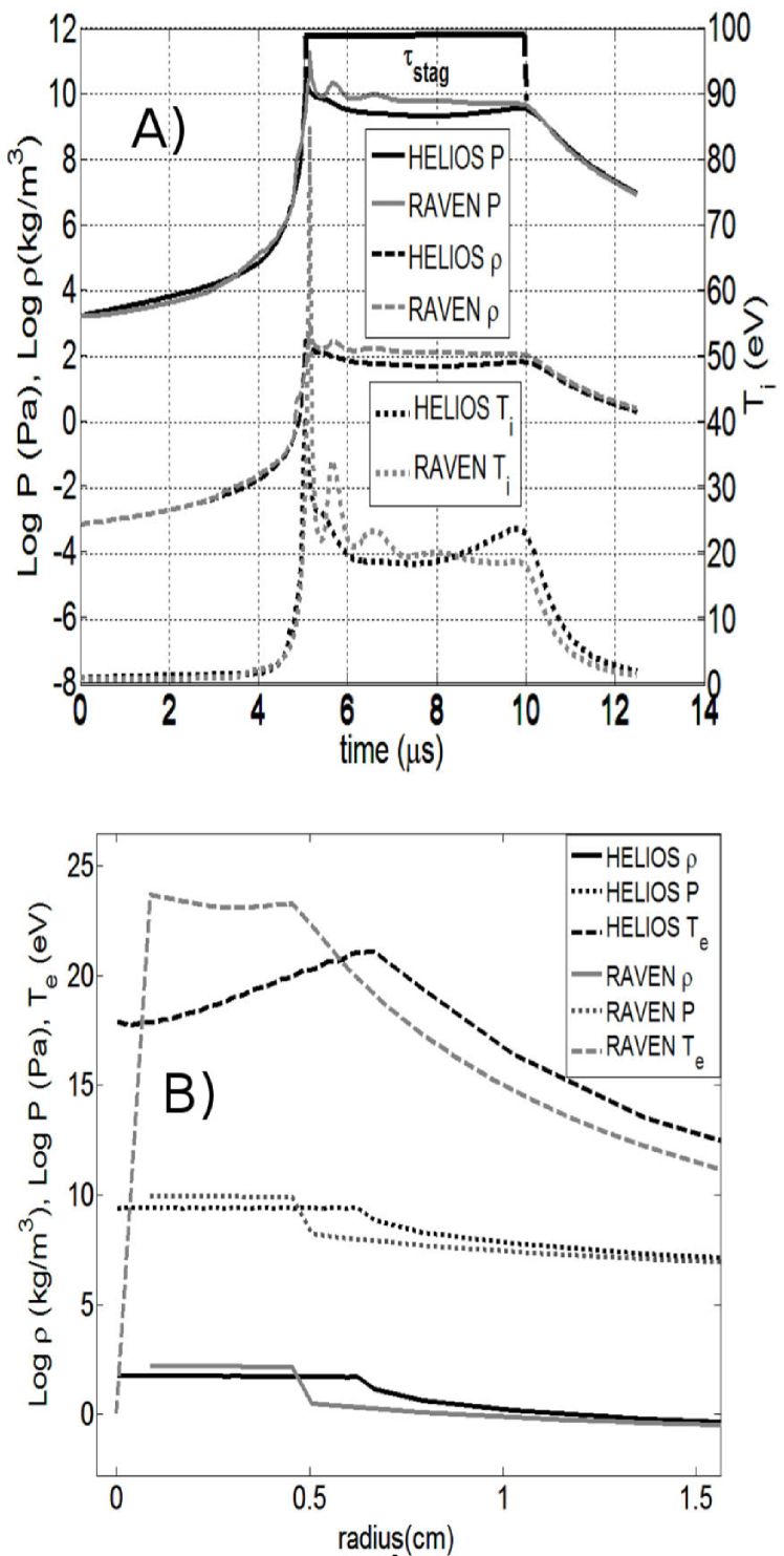
We compared the quantities and , where is defined as the thermal pressure in the simulation zone that is initially 1.0 mm from the inner edge of the liner ( cm) averaged over a time duration , which is defined (and also shown graphically in Fig. 2A) as the time duration between maximum pressure to the time when pressure sustainment ends due to the outward going shock reaching the outer edge of the incoming liner. We found that RAVEN results (Table 2) are 1.2–3.5 times higher than the HELIOS-CR results (Table 3). The results agree to within 20%. These differences were considered to be small enough to proceed with this study.
We also compared HELIOS-CR and RAVEN simulation results for the time evolution (Fig. 2A) of the pressure , mass density , and ion temperature of a single computational zone (initially 1.0 cm from the inner edge of the liner, to be consistent with Fig. 4 of Awe et al.Awe et al. (2011)), and the radial profiles (Fig. 2B) of , , and electron temperature at a single time ( s), for run 6 of Table 1. Both comparisons indicate good qualitative agreement with some discrepancies. One difference is the increase in both and near the end of for the HELIOS-CR but not the RAVEN results. The magnitude of the rise in increases with increasing and is present throughout the entire stagnated liner, and is thus not a localized numerical effect in a single zone. The reason for this rise is not yet understood, but because this does not affect the conclusions of this paper, we have set the issue aside. There are also differences in the radial profiles at s, largely due to the slight difference in time evolution between the two simulations. At this time, there is an outward going shock for both the HELIOS-CR (at cm) and RAVEN (at cm) simulations, but the HELIOS-CR shock has propagated farther outward. The discrepancy in inside the shock also appears to be due to the difference in time evolution, as slightly later radial profiles from the RAVEN results also fall toward the origin (see Fig. 4 of Awe et al.Awe et al. (2011)). These differences do not affect the conclusions of this paper. The rest of the paper focuses on comparing HELIOS-CR simulations using a polytropic EOS versus tabular EOS data.
III Results
This section presents HELIOS-CR simulation results and analysis. Firstly, we discuss LTE versus non-LTE tabular EOS results, showing that there are only minor differences, thus justifying our choice to focus on the use of LTE for the subsequent results in the paper. Secondly, we compare argon plasma liner implosions between polytropic and a LTE tabular EOS to assess the effects of ionization and a more sophisticated treatment of EOS. Finally, we explore the effects of using different plasma liner species for run 6 of Table 1, again using LTE tabular EOS data.
III.1 LTE versus Non-LTE EOS tabular data
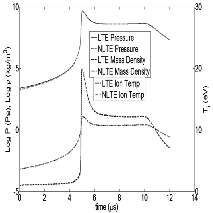
The initial conditions we used (see Table 1) are in a parameter space in which LTE is not obviously correct. Non-LTE can have an effect on EOS (i.e., ionization/excitation) and radiation losses (excited states tend to be less populated). Below an argon ion density of cm-3 at eV, the fractions of Ar I, Ar II, and Ar III as a function of temperature are noticeably different between LTE and non-LTE calculations. Above cm-3, corresponding to later stages of liner implosion and stagnation, the EOS data are similar. We performed run 6 of Table 1 using both LTE and non-LTE tabular EOS data to explicitly assess the difference in results. Figure 3 shows a comparison of , , and versus time for the computational zone that is initially 1.0 cm from the inside edge of the plasma liner. Note that for the tabular EOS runs, the pressure is calculated as , where and are the ion and electron densities, respectively, , and is the mean charge state. The LTE and non-LTE results are virtually indistinguishable over the entire duration of the simulation, and there are also no appreciable differences in , , and over the entire liner at several time steps (not shown). This indicates that either LTE or non-LTE EOS models could be used without altering the relevant simulation results for the purposes of this study, and thus we used LTE for all subsequent results presented in the paper.
III.2 Tabular LTE EOS versus polytropic EOS
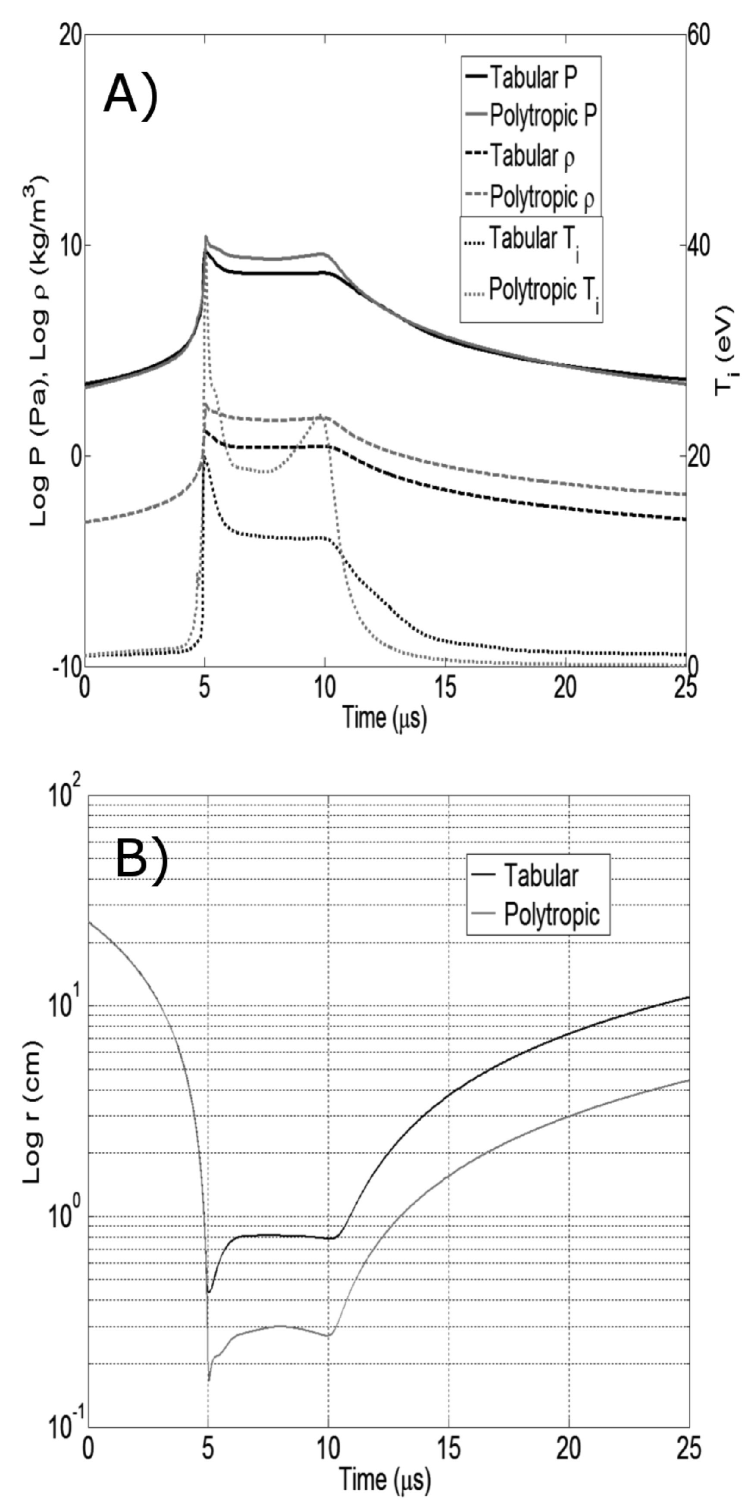
To assess the effects of ionization and other effects included in the LTE tabular EOS data, we compared HELIOS-CR simulation results using LTE tabular EOS with those using a polytropic () EOS for runs 1–8 of Table 1. For the computational zone that is initially 1.0 mm from the inside edge of the liner, the maximum pressure is 3.6–6.1 times larger and 3.9–8.6 times larger for the polytropic EOS results. Complete results for both the tabular LTE and polytropic EOS’s are shown in Tables 1 and 3, respectively. The and at peak compression were also higher in the polytropic EOS results as well (not shown). Figure 4 shows , , , and radial position versus time of the computational zone initially at 25.1 cm (1.0 cm from the inside edge of the liner) for the initial conditions of run 6 of Table 1. The lower ( zone thermal energy divided by zone volume) for the tabular EOS result is consistent with the combined effects of lower zone thermal energy () and higher zone volume at peak compression, as compared to the polytropic result. Next, we investigate in more detail the reasons for the lower zone thermal energy and higher zone volume at peak compression for the tabular EOS run.
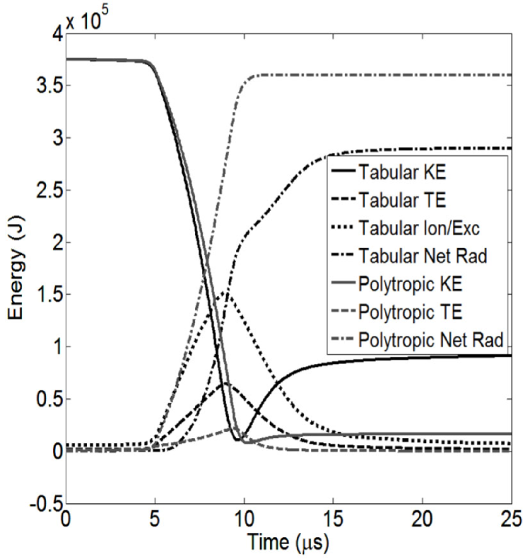
Figure 5 shows various components of the total liner energy versus time for run 6 of Table 1. The liner kinetic energy falls quickly around 5 s when the leading edge of the liner reaches peak compression and stagnates. In the polytropic EOS case, the difference between the initial and the stagnated liner thermal energy is due mostly to radiative losses. In the tabular EOS case, around half of the initial liner goes to ionization/excitation energy, which is stored in free and excited electrons in the stagnated liner. The mean charge peaks around 7 (see Sec. III.4). The result of including the ionization/excitation physics is a drastic reduction in the liner compression at stagnation, leading to lower (see Tables 1 and 3).
III.3 Stagnation pressure scalings
Awe et al.Awe et al. (2011) found the approximate scalings and for the cases in Table 1 using a polytropic EOS model, and gave an heuristic argument for why ought to be an upper bound on the scaling dependence of on . The heuristic argument invoked the following assumptions: (1) perfect conversion of liner to liner at stagnation, (2) no radiation and thermal losses, and (3) no entropy production due to the outward going post-stagnation shock. Because the RAVEN runs of Awe et al.Awe et al. (2011) included radiation and thermal losses, the observed weaker scaling is consistent with the heuristic upper bound of . Our HELIOS-CR runs using a LTE tabular EOS violate assumption (1) above due to the major ionization/excitation energy channel discussed in Sec. III.2. Thus, it is expected we should see an even weaker scaling than .
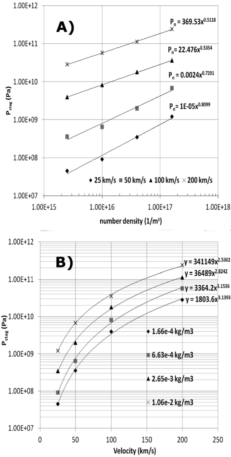
Figure 6 shows versus and and fits to power law functions for HELIOS-CR simulations of the cases in Table I using a LTE tabular EOS model. While the fitted exponents are very similar across density and velocity groups in Awe et al.,Awe et al. (2011) i.e., and , our fitted exponents have a much wider spread, i.e., and . This larger spread in exponents is likely due to the fact that the LTE tabular EOS is sensitive to density and temperature in the imploding plasma liner, thus introducing a degree of variability that depends on the liner initial conditions not expected in the polytropic EOS simulations of Awe et al.Awe et al. (2011) Our scaling (depending on ) is indeed weaker than the approximate scaling of Awe et al.,Awe et al. (2011) as expected. Our scaling agrees with the scaling of Awe et al.Awe et al. (2011) within our observed variation across velocity groups.
III.4 Varying the liner species
Due to the significant effect of ionization/excitation on achievable , we explored the use of different plasma species for the same initial liner and (and hence ) of run 6 of Table 1. The only quantity that was varied was the initial number density to keep constant. We performed HELIOS-CR simulations with LTE tabular EOS data to investigate the effect of species on . The species chosen for study are those of interest as fusion fuel, blanket materials, or MIF implosion drivers for fusion energy applications: H, D-T (50%-50% by atom), 4He, 6Li, 11B, Ne, Ar, Kr, and Xe.
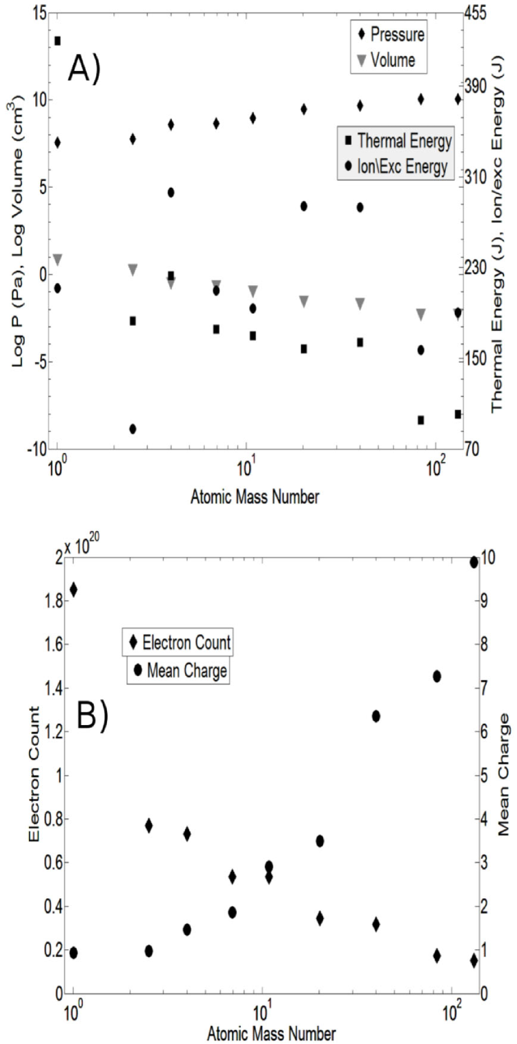
Figure 7A shows HELIOS-CR simulation results using a LTE tabular EOS model for , volume, , and ionization/excitation energy at peak compression versus atomic mass number for the zone initially 1.0 cm from the inner edge of the liner. There is a clear trend of increasing peak with atomic mass number, quantitatively consistent with the combined effects of decreasing volume and thermal pressure with atomic mass number at peak compression. The thermal and ionization/excitation energies are not monotonic with atomic mass number, and this is related to the different atomic and radiative properties of the different species.
We also examined the mean charge and electron count versus time (Fig. 7B) for the same computational zone as above. Although the heavier species have more electrons to ionize, there are a larger number of the lighter species present by the ratio of their atomic mass numbers. It turns out that the peak mean charge for the heavier species reaches only about 5–10 (Fig. 7B), much less than the mass ratios between the heavier and lighter species, and thus the electron count is higher for the lighter species. Thus, the ionization/excitation energies are in general higher for the lighter species, in part explaining why they reach lower peak pressures for the initial conditions imposed.
IV Discussion and summary
It appears that the key effect of using a LTE tabular EOS rather than a polytropic EOS is the significant diversion of liner into ionization/excitation, which is not included in the polytropic EOS model. The diversion of initial liner leads to less effective compression, larger minimum volume at peak compression, and thus lower which is inversely proportional to volume. This is detrimental for reaching very high peak temperatures and pressures in targetless spherical plasma liner implosions, which was one of the design objectives of PLX. For a given initial liner , which is a natural experimental constraint, the results suggest the use of lower density and higher velocity to achieve higher peak pressure. The previous statement is confirmed by examining, e.g., the results from runs 3, 6, and 9 (375 kJ), or runs 4, 7, 10, and 13 (1.5 MJ) of Table 1. Higher velocity should also be coupled with the use of lower atomic mass number species so as to fully strip the ions and eliminate the ionization/excitation and line radiation energy channels beyond a certain point in the implosion, after which the liner will predominantly go toward stagnation thermal pressure. This is in apparent contradiction with the results of Sec. III.4, which suggest the use of heavier species for higher but only because we constrained the species comparison study by enforcing the same and . In our species comparison study, the much higher of the lighter species leads to more of the initial liner going into ionization/excitation. Further study is needed for optimizing in targetless spherical plasma liner implosions for a given initial liner .
The above discussion does not apply for the MIF application of a plasma liner compressing a magnetized D-T target plasma.Hsu et al. (2012) In that case, the imploding plasma liner is intended to be only a pusher that should complete its job of compressing the D-T target to fusion conditions before the liner itself has a chance to get significantly compressed and heated. Thus, for initial liner and that are likely to be limited by available plasma gun technology, the MIF application likely will prefer a heavy liner species (to maximize ) since the ionization/excitation should not matter until after the D-T target has reached peak compression.
In summary, we have presented new 1D HELIOS-CR radiation-hydrodynamic simulation results of spherical plasma liners imploding on vacuum using a LTE tabular EOS model. The results were compared in detail to HELIOS-CR simulations using a polytropic EOS model (), which in turn were benchmarked against the polytropic EOS simulation results of Awe et al.Awe et al. (2011) We found that the liner stagnation pressure is lower by a factor of 3.9–8.6 using the LTE tabular EOS model. This is attributed to a significant amount of the initial liner kinetic energy going toward ionization/excitation of the plasma liner, resulting in less effective compression of the liner. We also studied the effect of different species on for the same initial liner geometry, mass density, and velocity. We found that with these constraints, the heaviest species reach the highest values of . This is attributed to less total energy going to ionization/excitation due to a smaller value at peak compression of the liner mean charge times the initial number density.
Acknowledgements.
The authors thank T. J. Awe for access to the RAVEN simulation data. This work was supported by the Office of Fusion Energy Sciences of the U.S. Department of Energy.References
- Hsu et al. (2012) S. C. Hsu, T. J. Awe, S. Brockington, A. Case, J. T. Cassibry, G. Kagan, S. J. Messer, M. Stanic, X. Tang, D. R. Welch, and F. D. Witherspoon, IEEE Trans. Plasma Sci. 40, 1287 (2012).
- Thio et al. (1999) Y. C. F. Thio, E. Panarella, R. C. Kirkpatrick, C. E. Knapp, F. Wysocki, P. Parks, and G. Schmidt, in Current Trends in International Fusion Research–Proceedings of the Second International Symposium, edited by E. Panarella (National Research Council of Canada, Ottawa, 1999).
- Thio et al. (2001) Y. C. F. Thio, C. E. Knapp, R. C. Kirkpatrick, R. E. Siemon, and P. J. Turchi, J. Fusion Energy 20, 1 (2001).
- Lindemuth and Kirkpatrick (1983) I. R. Lindemuth and R. C. Kirkpatrick, Nucl. Fusion 23, 263 (1983).
- Kirkpatrick, Lindemuth, and Ward (1995) R. C. Kirkpatrick, I. R. Lindemuth, and M. S. Ward, Fusion Tech. 27, 201 (1995).
- Lindemuth and Siemon (2009) I. R. Lindemuth and R. E. Siemon, Amer. J. Phys. 77, 407 (2009).
- Awe et al. (2011) T. J. Awe, C. S. Adams, J. S. Davis, D. S. Hanna, S. C. Hsu, and J. T. Cassibry, Phys. Plasmas 18, 072705 (2011).
- Parks (2008) P. B. Parks, Phys. Plasmas 15, 062506 (2008).
- Cassibry et al. (2009) J. T. Cassibry, R. J. Cortez, S. C. Hsu, and F. D. Witherspoon, Phys. Plasmas 16, 112707 (2009).
- Samulyak, Parks, and Wu (2010) R. Samulyak, P. Parks, and L. Wu, Phys. Plasmas 17, 092702 (2010).
- Santarius (2012) J. F. Santarius, Phys. Plasmas 19, 072705 (2012).
- MacFarlane, Golovkin, and Woodruff (2006) J. J. MacFarlane, I. E. Golovkin, and P. R. Woodruff, J. Quant. Spect. Rad. Transfer 99, 381 (2006).
- Cassibry et al. (2012) J. T. Cassibry, M. Stanic, S. C. Hsu, F. D. Witherspoon, and S. I. Abarzhi, Phys. Plasmas 19, 052702 (2012).
- Witherspoon et al. (2011) F. D. Witherspoon, S. Brockington, A. Case, S. J. Messer, L. Wu, R. Elton, S. C. Hsu, J. T. Cassibry, and M. A. Gilmore, Bull. Amer. Phys. Soc. 56, 311 (2011).
- Kagan et al. (2011) G. Kagan, X. Tang, S. C. Hsu, and T. J. Awe, Phys. Plasmas 18, 120702 (2011).
- MacFarlane et al. (2005) J. J. MacFarlane, I. E. Golovkin, R. C. Mancini, L. A. Welser, J. E. Bailey, J. A. Koch, T. A. Mehlhorn, G. A. Rochau, P. Wang, and P. Woodruff, Phys. Rev. E 72, 066403 (2005).
- Welser-Sherrill et al. (2007) L. Welser-Sherrill, R. C. Mancini, J. A. Koch, N. Izumi, R. Tommasini, S. W. Haan, D. A. Haynes, I. E. Golovkin, J. J. MacFarlane, J. A. Delettrez, F. J. Marshall, S. P. Regan, V. A. Smalyuk, and G. Kyrala, Phys. Rev. E 76, 056403 (2007).
- More et al. (1988) R. M. More, K. H. Warren, D. A. Young, and G. B. Zimmerman, Phys. Fluids 31, 3059 (1988).
- Noh (1987) W. F. Noh, J. Comp. Phys. 72, 78 (1987).
- Oliphant (1981) T. A. Oliphant, “RAVEN Physics Manual,” Tech. Rep. LA-8802-M (Los Alamos National Laboratory, NM, 1981).
| Run | (cm-3) | (kg/m3) | (km/s) | (J) | (s) | (Pa) | (Pa) | ||
|---|---|---|---|---|---|---|---|---|---|
| 1 | 2.5E+15 | 1.66E-4 | 25 | 2.35E+4 | 9.40 | 4.49E+07 | 1.31E+08 | 4.22E+2 | 0.018 |
| 2 | 2.5E+15 | 1.66E-4 | 50 | 9.39E+4 | 5.35 | 3.54E+08 | 1.84E+09 | 1.90E+3 | 0.020 |
| 3 | 2.5E+15 | 1.66E-4 | 100 | 3.76E+5 | 2.70 | 3.93E+09 | 1.43E+10 | 1.06E+4 | 0.028 |
| 4 | 2.5E+15 | 1.66E-4 | 200 | 1.50E+6 | 1.30 | 2.84E+10 | 5.69E+10 | 3.69E+4 | 0.025 |
| 5 | 1.0E+16 | 6.63E-4 | 25 | 9.38E+4 | 9.55 | 9.15E+07 | 3.57E+08 | 8.74E+2 | 0.093 |
| 6 | 1.0E+16 | 6.63E-4 | 50 | 3.75E+5 | 5.35 | 6.43E+08 | 4.63E+09 | 3.44E+3 | 0.092 |
| 7 | 1.0E+16 | 6.63E-4 | 100 | 1.50E+6 | 2.70 | 8.20E+09 | 3.13E+10 | 2.21E+4 | 0.015 |
| 8 | 1.0E+16 | 6.63E-4 | 200 | 6.00E+6 | 1.35 | 5.70E+10 | 1.26E+11 | 7.40E+4 | 0.013 |
| 9 | 4.0E+16 | 2.65E-3 | 25 | 3.75E+5 | 10.45 | 3.47E+08 | 1.43E+09 | 3.62E+3 | 0.010 |
| 10 | 4.0E+16 | 2.65E-3 | 50 | 1.50E+6 | 5.45 | 2.00E+09 | 1.43E+10 | 1.09E+4 | 0.007 |
| 11 | 4.0E+16 | 2.65E-3 | 100 | 6.00E+6 | 2.70 | 1.79E+10 | 1.30E+11 | 4.83E+4 | 0.008 |
| 12 | 4.0E+16 | 2.65E-3 | 200 | 2.40E+7 | 1.35 | 1.13E+11 | 7.39E+11 | 1.53E+5 | 0.006 |
| 13 | 1.6E+17 | 1.06E-2 | 25 | 1.50E+6 | 10.50 | 1.23E+09 | 4.97E+09 | 1.29E+4 | 0.009 |
| 14 | 1.6E+17 | 1.06E-2 | 50 | 6.00E+6 | 5.70 | 6.81E+09 | 6.02E+10 | 3.88E+4 | 0.006 |
| 15 | 1.6E+17 | 1.06E-2 | 100 | 2.40E+7 | 2.70 | 3.56E+10 | 4.27E+11 | 9.61E+4 | 0.004 |
| 16 | 1.6E+17 | 1.06E-2 | 200 | 9.59E+7 | 1.35 | 2.40E+11 | 2.23E+12 | 3.24E+5 | 0.003 |
| Run | (s) | (Pa) | (Pa) | ||
|---|---|---|---|---|---|
| 1 | 8.82 | 2.37E+08 | 3.17E+9 | 2.09E+3 | 0.09 |
| 2 | 4.51 | 3.11E+09 | 8.58E+10 | 1.40E+4 | 0.15 |
| 3 | 2.29 | 3.43E+10 | 8.82E+11 | 7.84E+4 | 0.21 |
| 4 | 1.03 | 6.29E+11 | 4.26E+13 | 6.48E+5 | 0.43 |
| 5 | 8.84 | 4.78E+08 | 4.41E+09 | 4.23E+3 | 0.05 |
| 6 | 4.56 | 6.79E+09 | 1.32E+11 | 3.09E+4 | 0.08 |
| 7 | 2.33 | 8.39E+10 | 2.40E+12 | 1.95E+5 | 0.13 |
| 8 | 1.19 | 8.32E+11 | 2.35E+13 | 9.86E+5 | 0.16 |
| Run | (s) | (Pa) | (Pa) | ||
|---|---|---|---|---|---|
| 1 | 10.30 | 1.73E+08 | 7.44E+08 | 1.79E+3 | 0.08 |
| 2 | 5.05 | 1.87E+09 | 1.09E+10 | 9.44E+3 | 0.10 |
| 3 | 2.55 | 1.63E+10 | 5.15E+10 | 4.16E+4 | 0.11 |
| 4 | 1.30 | 1.78E+11 | 3.19E+11 | 2.32E+5 | 0.15 |
| 5 | 11.15 | 3.91E+08 | 1.64E+09 | 4.36E+3 | 0.05 |
| 6 | 5.05 | 4.11E+09 | 2.71E+10 | 2.08E+4 | 0.06 |
| 7 | 2.65 | 7.09E+10 | 1.54E+11 | 1.88E+5 | 0.13 |
| 8 | 1.30 | 3.86E+11 | 7.70E+11 | 5.02E+5 | 0.08 |