Online Adversarial Stabilization of
Unknown Linear Time-Varying Systems

We study the dynamics in (1) and make the following standard assumptions about the dynamics.

Bounded and non-stochastic (potentially adversarial) disturbances is a common model both in the online learning and control problems [39, 40]. Since we make no assumptions on how large the bound $W$ is, 1 models a variety of scenarios, such as bounded and/or correlated stochastic noise, state-dependent disturbances, e.g., the linearization and discretization error for nonlinear continuous-time dynamics, and potentially adversarial disturbances. 2 is standard in learning-based control, e.g. [41, 42].

We additionally assume there is a quadratic known cost function of the state and control input at every time step $t$ to be minimized, e.g. $x_{t}^{\top}Qx_{t}+u_{t}^{\top}Ru_{t}$, with $Q,\,R\succ 0$. For a given LTI system model $\theta=[A\ B]$ and cost matrices $Q,\,R$, we denote $K=\textsc{LQR}(\theta;Q,R)$ as the optimal feedback gain for the corresponding infinite-horizon LQR problem.

Convex Body Chasing (CBC) is a well-studied online learning problem [35, 36]. At every round $t\in\mathbb{N}_{+}$, the player is presented a convex body/set $\mathcal{K}_{t}\subset\mathbb{R}^{n}$. The player selects a point $q_{t}\in\mathcal{K}_{t}$ with the objective of minimizing the cost defined as the total path length of the selection for $T$ rounds, e.g., $\sum_{t=1}^{T}\|q_{t}-q_{t-1}\|$ for a given initial condition $q_{0}\not\in\mathcal{K}_{1}$. There are many known algorithms for the CBC problem with a competitive ratio guarantee such that the cost incurred by the algorithm is at most a constant factor from the total path length incurred by the offline optimal algorithm which has the knowledge of the entire sequence of the bodies. We will use CBC to select $\theta_{t}$’s that are consistent with observed data.

The main result of this paper is the BIBO stability guarantee for Algorithm 1 in terms of the true model variation and the disturbance bound. We sketch the proof in this section and refer Section -C for the formal proof. This result depends on a refined analysis of the competitive ratio for the functional Steiner point chasing algorithm introduced in [33], which is stated as follows.

Proof Sketch: At a high level, the structure of our proof is as follows. We first use the fact that our time-varying feedback gain $\widehat{K}_{t}$ is computed according to a hypothesis model from the consistent model set. Therefore, we can characterize the closed-loop dynamics in terms of the consistent models $\widehat{\theta}_{t}$ and $\widehat{K}_{t}$. Specifically, consider a time step $t$ where we take the action $u_{t}=\widehat{K}_{t-1}x_{t}$ after observing $x_{t}$. Then, we observe $x_{t+1}=A_{t}x_{t}+B_{t}u_{t}+w_{t}$ and select a new hypothesis model $\widehat{\theta}_{t}=[\widehat{A}_{t}\ \widehat{B}_{t}]$ that is consistent with this new observation. Since we have selected a consistent hypothesis model, there is some admissible disturbance $\widehat{w}_{t}$ satisfying 1 such that

Without loss of generality, we assume initial condition $x_{0}=0$. We therefore have

We have two main challenges in bounding $\left\|x_{t}\right\|$ in (6):

1. 1.

   $\widehat{K}_{t}$ is computed using $\widehat{\theta}_{t}$ in Algorithm 1, but is applied to the next time step $\widehat{\theta}_{t+1}$. While we know $\rho(\widehat{A}_{t}+\widehat{B}_{t}\widehat{K}_{t})<1$, in (6) we have $\widehat{K}_{t-1}$ instead of $\widehat{K}_{t}$.

2. 2.

   Naively applying submultiplicativity of the operator norm for (6) results in bounding $\left\|\left(\widehat{A}_{\tau}+\widehat{B}_{\tau}\widehat{K}_{\tau-1}\right)\right\|$. However, even if $\widehat{K}_{t-1}$ satisfies $\rho(\widehat{A}_{t}+\widehat{B}_{t}\widehat{K}_{t})<1$, in general the operator norm can be greater than 1.

To address the first challenge, our key insight is that by selecting hypothesis models via CBC technique, in any interval where the true model variation is small, our selected hypothesis model also vary little. Specifically, by Lemma 1, we can bound the partial-path variation of the selected hypothesis models with the true model partial-path variation $\Delta_{[s,e]}$ as follows.

where $\Theta$ and $\kappa$ are from 2. A consequence of (7) is that, during intervals where the true model variation is small, we have $\left(\widehat{A}_{t}+\widehat{B}_{t}\widehat{K}_{t-1}\right)\approx\left(\widehat{A}_{t}+\widehat{B}_{t}\widehat{K}_{t}\right)$.

For the second challenge, we leverage the concept of sequential strong stability [43], which allows bounding $\left\|\prod_{\tau\in[t-1:s+1]}\left(\widehat{A}_{\tau}+\widehat{B}_{\tau}\widehat{K}_{\tau-1}\right)\right\|$ approximately with $\prod_{\tau\in[t-1:s+1]}\rho\left(\widehat{A}_{\tau}+\widehat{B}_{\tau}\widehat{K}_{\tau}\right)$ times $\mathcal{O}\left(\exp(\Delta_{[s,t-1]})\right)$.

We now sketch the proof. The helper lemmas are summarized in Section -B and the formal proof can be found in Section -C. Consider $L_{t},\,H_{t}\in\mathbb{R}^{n\times n}$ with $H_{t}\succ 0$ such that

We use $I_{s}$ as shorthand for the interval $[t-1:s+1]$. Then each summand in (6) can be bounded as

Therefore showing BIBO stability comes down to bounding individual terms in (8). In particular we will show that by selecting appropriate $H_{t}$ and $L_{t}$, term (a) is bounded by a constant $C_{H}$ that depends on system theoretical properties of the worst-case parameter in $\Theta$. For (b) and (c), we isolate the instances when

for some chosen $\epsilon>0$. For instances where (9) holds, we use the perturbation analysis of the Lyapunov equation involving the matrix $\widehat{A}_{t}+\widehat{B}_{t}\widehat{K}_{t-1}$ (Lemma 6 for (b) and Lemma 4 for (c)) to bound (b) and (c) in terms of the partial-path movement of the selected parameters $\widehat{\Delta}_{[s,e]}:=\sum_{\tau=s+1}^{e}\left\|\textsf{st}(\omega_{\tau+1})-\textsf{st}(\omega_{\tau})\right\|_{F}$. Specifically, Lemma 6 implies

where $\beta,\,\bar{H}>1$ are constants. We also show that from Lemma 4,

for $\rho_{L}\in(0,1)$ and $\bar{L}>1$ a constant.

We now plug (10) and (11) into (8). Denote by $n_{[s,t]}$ the number of pairs $(\tau,\tau-1)$ with $s+1\leq\tau\leq t-1$ where (9) fails to hold. Let ${\Delta}_{[s,e]}:=\sum_{\tau=s+1}^{e}\left\|\theta_{\tau}-\theta_{\tau-1}\right\|_{F}$ be the true model partial-path variation. Then (8) can be bounded as

for constants $c,\,c_{2}$ and $\bar{n}:=n(n+m)$ for the dimension of the parameter space for $A_{t},\,B_{t}$. In the second inequality, we used the observation that $n_{[s,t]}\leq\frac{\widehat{\Delta}_{[s,t-1]}}{\epsilon}$ and in the last inequality we used Lemma 1. Combined with (6) and 1, this proves the desired bound. $\blacksquare$

An immediate consequence of Theorem 1 is that when the model variation in (1) is bounded or sublinear, Algorithm 1 guarantees BIBO stability. This is summarized below.

Corollary 1 can be useful for scenarios where the mode of operation of the system changes infrequently and for systems such that $\theta(t)\rightarrow\theta^{\star}$ as $t\rightarrow\infty$ [44]. As an example, consider power systems where a prescribed set of lines can potentially become disconnected from the grid and thus change the grid topology. Corollary 2 applies to slowly drifting systems [45].

In general, implementation of the functional Steiner point of the work function may be computationally inefficient. However, by taking advantage of the LTV structure, we are able to design an efficient implementation in our setting. The key observation here is that for each $t$, $\mathcal{P}_{t}$ (Algorithm 1, line 1) can be described by the intersection of half-spaces because the ambient parameter space $\Theta$ is assumed to be a polytope and the observed online transition data from $x_{t},\,u_{t}$ to $x_{t+1}$ specifies two half-space constraints at each time step due to linearity of (1). Our approach to approximate the functional Steiner point for chasing the consistent model sets is inspired by [34] where second-order cone programs (SOCPs) are used to approximate the (nested set) Steiner point of the sublevel set of the work functions for chasing half-spaces.

Denote $\{(a_{i},b_{i})\}_{i=1}^{p_{t}}$ as the collection of $p_{t}$ half-space constraints describing $\mathcal{P}_{t}$, i.e., $a_{i}^{\top}\theta\leq b_{i}$. To approximate the integral for the functional Steiner point (2) of $\omega_{t}$, we sample $N$ number of random directions $v\in\mathbb{S}^{n-1}$, evaluate the Fenchel conjugate of the work function $\omega^{*}_{t}$ at each $v$ with an SOCP, and take the empirical average. Finally we project the estimated functional Steiner point back to the set of consistent model $\mathcal{P}_{t}\cap\Theta$. Even though the analytical functional Steiner point (2) is guaranteed to be a member of the consistent model set, the projection step is necessary because we are integrating numerically, which may result in an approximation that ends up outside of the set. We summarize this procedure in Algorithm 2. Specifically, given a direction $v\in\mathbb{S}^{n-1}$, the Fenchel conjugate of the work function at time step $t$ is

This can be equivalently expressed as the following SOCP with decision variables $x,q_{1},\ldots,q_{t},\lambda,\lambda_{1},\ldots,\lambda_{t}$:

Another potential implementation challenge is that the number of constraints in the SOCP (12) grows linearly with time due to the construction of the work function (4). This is a common drawback of online control methods based on CBC and NCBC techniques and can be overcome through truncation or over-approximation in of the work functions in practice. Additionally, if the LTV system is periodic with a known period, then we can leverage Algorithm 1 during the initial data collection phase. Once representative (persistently exciting) data is available, one could employ methods like [3] to generate a stabilizing controller for the unknown LTV system. In Section IV, we show that data collection via Algorithm 1 results in a significantly smaller state norm than random noise injection when the system is unstable.

We consider the following Markov linear jump system (MLJS) model from [46], with

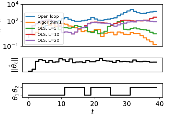
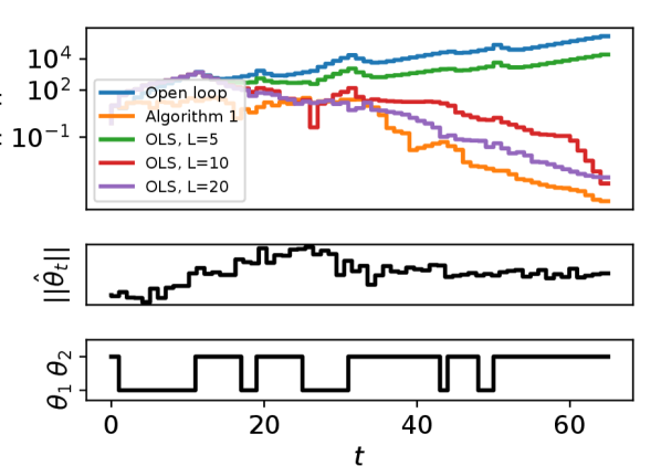
where $\Pi$ is the transition probability matrix from $\theta_{1}$ to $\theta_{2}$ and vice versa. We inject uniformly random disturbances such that $w_{t}\in\{-10\mathds{1},\,-3\mathds{1},\,3\mathds{1}\}$ where $\mathds{1}$ is the all-one vector. We set the disturbances to be zero for the last 10 time steps to make explicit the stability of the closed loop. We implement certainty-equivalent control based on online least squares (OLS) with different sliding window sizes $L=5,\,10,\,20$ and a exponential forgetting factor of $0.95$ [47] as the baselines.

We show two different MLJS models generated from 2 random seeds and show the results in Figure 1. For both systems, the open loop is unstable. In Figure 1(a) the OLS-based algorithms fail to stabilize the system for window size of $L=20$, while stabilizing the system but incurring larger state norm than the proposed algorithm for $L=5,\,10$. On the other hand, in Figure 1(b), OLS with $L=5$ results in unstable closed loop. This example highlights the challenge of OLS-based methods, where the choice of window size is crucial for the performance. Since the underlying LTV system is unknown and our goal is to control the system online, it is unclear how to select appropriate window size to guarantee stability for OLS-based methods a priori. In contrast, Algorithm 1 does not require any parameter tuning.

We note that while advanced least-squares based identification techniques that incorporate sliding window with variable length exist, e.g. [4, 47], due to the unknown system parameters, it is unclear how to choose the various algorithm parameters such as thresholds for system change detection. Therefore, we only compare Algorithm 1 against fixed-length sliding window OLS methods as baselines.

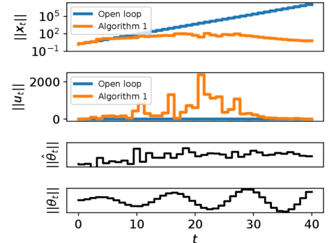
Our second example highlights that Algorithm 1 is a useful data-collection alternative to open-loop random noise injection. We consider the LTV system from [3, 28], with

where we modified $A(1,1)$ from 1 to 1.5 to increase the instability of the open loop in the beginning; thus making it more challenging to stabilize. We consider no disturbances here, which is a common setting in direct data-driven control, e.g., [3, 26, 27]. In particular, we compare the proposed algorithm against randomly generated bounded inputs from $\textsf{UNIF}[-1,1]$. We also modify the control inputs from Algorithm 1 to be $u_{t}=\widehat{K}_{t-1}x_{t}+\eta_{t}\cdot\mathds{1}$ with $\eta_{t}\sim\textsf{UNIF}[-1,1]$ so that we can collect rich data in the closed loop. This is motivated by the growing body of data-driven control methods such as [3, 27, 28] that leverage sufficiently rich offline data to perform control design for unknown LTV systems. However, most of these works directly inject random inputs for data collection. It is evident in Figure 2 that when the open-loop system is unstable it may be undesirable to run the system without any feedback control. Therefore, Algorithm 1 complements existing data-driven methods by allowing safe data collection with significantly better transient behavior.

References

- [1] D. Deka, S. Backhaus, and M. Chertkov, “Structure learning in power distribution networks,” IEEE Transactions on Control of Network Systems, vol. 5, no. 3, pp. 1061–1074, Sep. 2018.
- [2] P. Gradu, E. Hazan, and E. Minasyan, “Adaptive regret for control of time-varying dynamics,” arXiv preprint arXiv:2007.04393, 2020.
- [3] B. Nortmann and T. Mylvaganam, “Data-driven control of linear time-varying systems,” in 2020 59th IEEE Conference on Decision and Control (CDC). IEEE, 2020, pp. 3939–3944.
- [4] Y. Luo, V. Gupta, and M. Kolar, “Dynamic regret minimization for control of non-stationary linear dynamical systems,” Proceedings of the ACM on Measurement and Analysis of Computing Systems, vol. 6, no. 1, pp. 1–72, 2022.
- [5] Y. Lin, J. Preiss, E. Anand, Y. Li, Y. Yue, and A. Wierman, “Online adaptive controller selection in time-varying systems: No-regret via contractive perturbations,” arXiv preprint arXiv:2210.12320, 2022.
- [6] E. Minasyan, P. Gradu, M. Simchowitz, and E. Hazan, “Online control of unknown time-varying dynamical systems,” Advances in Neural Information Processing Systems, vol. 34, pp. 15 934–15 945, 2021.
- [7] R. Tedrake, “Underactuated robotics: Learning, planning, and control for efficient and agile machines course notes for mit 6.832,” Working draft edition, vol. 3, p. 4, 2009.
- [8] P. Falcone, F. Borrelli, H. E. Tseng, J. Asgari, and D. Hrovat, “Linear time-varying model predictive control and its application to active steering systems: Stability analysis and experimental validation,” International Journal of Robust and Nonlinear Control: IFAC-Affiliated Journal, vol. 18, no. 8, pp. 862–875, 2008.
- [9] K. S. Tsakalis and P. A. Ioannou, Linear time-varying systems: control and adaptation. Prentice-Hall, Inc., 1993.
- [10] R. Tóth, Modeling and identification of linear parameter-varying systems. Springer, 2010, vol. 403.
- [11] J. Mohammadpour and C. W. Scherer, Control of linear parameter varying systems with applications. Springer Science & Business Media, 2012.
- [12] W. Zhang, Q.-L. Han, Y. Tang, and Y. Liu, “Sampled-data control for a class of linear time-varying systems,” Automatica, vol. 103, pp. 126–134, 2019.
- [13] R. Mojgani and M. Balajewicz, “Stabilization of linear time-varying reduced-order models: A feedback controller approach,” International Journal for Numerical Methods in Engineering, vol. 121, no. 24, pp. 5490–5510, 2020.
- [14] G. Goel and B. Hassibi, “Regret-optimal estimation and control,” IEEE Transactions on Automatic Control, 2023.
- [15] K. Tsakalis and P. Ioannou, “Adaptive control of linear time-varying plants,” Automatica, vol. 23, no. 4, pp. 459–468, 1987.
- [16] J.-J. Slotine and J. Coetsee, “Adaptive sliding controller synthesis for non-linear systems,” International Journal of Control, vol. 43, no. 6, pp. 1631–1651, 1986.
- [17] R. Marino and P. Tomei, “Adaptive control of linear time-varying systems,” Automatica, vol. 39, no. 4, pp. 651–659, 2003.
- [18] M. Verhaegen and X. Yu, “A class of subspace model identification algorithms to identify periodically and arbitrarily time-varying systems,” Automatica, vol. 31, no. 2, pp. 201–216, 1995.
- [19] B. Bamieh and L. Giarre, “Identification of linear parameter varying models,” International Journal of Robust and Nonlinear Control: IFAC-Affiliated Journal, vol. 12, no. 9, pp. 841–853, 2002.
- [20] T. Sarkar, A. Rakhlin, and M. Dahleh, “Nonparametric system identification of stochastic switched linear systems,” in 2019 IEEE 58th Conference on Decision and Control (CDC), 2019.
- [21] S. Dean, S. Tu, N. Matni, and B. Recht, “Safely learning to control the constrained linear quadratic regulator,” in 2019 American Control Conference (ACC). IEEE, 2019, pp. 5582–5588.
- [22] S. Talebi, S. Alemzadeh, N. Rahimi, and M. Mesbahi, “On regularizability and its application to online control of unstable lti systems,” IEEE Transactions on Automatic Control, 2021.
- [23] S. Lale, K. Azizzadenesheli, B. Hassibi, and A. Anandkumar, “Reinforcement learning with fast stabilization in linear dynamical systems,” in International Conference on Artificial Intelligence and Statistics. PMLR, 2022, pp. 5354–5390.
- [24] J. Yu, D. Ho, and A. Wierman, “Online adversarial stabilization of unknown networked systems,” Proceedings of the ACM on Measurement and Analysis of Computing Systems, vol. 7, no. 1, pp. 1–43, 2023.
- [25] X. Chen and E. Hazan, “Black-box control for linear dynamical systems,” in Conference on Learning Theory. PMLR, 2021.
- [26] M. Rotulo, C. De Persis, and P. Tesi, “Online learning of data-driven controllers for unknown switched linear systems,” Automatica, vol. 145, p. 110519, 2022.
- [27] S. Baros, C.-Y. Chang, G. E. Colon-Reyes, and A. Bernstein, “Online data-enabled predictive control,” Automatica, vol. 138, p. 109926, 2022.
- [28] B. Pang, T. Bian, and Z.-P. Jiang, “Data-driven finite-horizon optimal control for linear time-varying discrete-time systems,” in 2018 IEEE Conference on Decision and Control (CDC), 2018, pp. 861–866.
- [29] S.-J. Liu, M. Krstic, and T. Başar, “Batch-to-batch finite-horizon lq control for unknown discrete-time linear systems via stochastic extremum seeking,” IEEE Transactions on Automatic Control, vol. 62, no. 8, pp. 4116–4123, 2016.
- [30] G. Qu, Y. Shi, S. Lale, A. Anandkumar, and A. Wierman, “Stable online control of linear time-varying systems,” in Learning for Dynamics and Control. PMLR, 2021, pp. 742–753.
- [31] Y. Ouyang, M. Gagrani, and R. Jain, “Learning-based control of unknown linear systems with thompson sampling,” arXiv preprint arXiv:1709.04047, 2017.
- [32] Y. Han, R. Solozabal, J. Dong, X. Zhou, M. Takac, and B. Gu, “Learning to control under time-varying environment,” arXiv preprint arXiv:2206.02507, 2022.
- [33] M. Sellke, “Chasing convex bodies optimally,” in Proceedings of the Fourteenth Annual ACM-SIAM Symposium on Discrete Algorithms. SIAM, 2020, pp. 1509–1518.
- [34] C. Argue, A. Gupta, Z. Tang, and G. Guruganesh, “Chasing convex bodies with linear competitive ratio,” Journal of the ACM (JACM), vol. 68, no. 5, pp. 1–10, 2021.
- [35] N. Bansa, M. Böhm, M. Eliáš, G. Koumoutsos, and S. W. Umboh, “Nested convex bodies are chaseable,” in Proceedings of the Twenty-Ninth Annual ACM-SIAM Symposium on Discrete Algorithms. SIAM, 2018, pp. 1253–1260.
- [36] S. Bubeck, B. Klartag, Y. T. Lee, Y. Li, and M. Sellke, “Chasing nested convex bodies nearly optimally,” in Proceedings of the Fourteenth Annual ACM-SIAM Symposium on Discrete Algorithms. SIAM, 2020.
- [37] D. Ho, H. Le, J. Doyle, and Y. Yue, “Online robust control of nonlinear systems with large uncertainty,” in International Conference on Artificial Intelligence and Statistics. PMLR, 2021, pp. 3475–3483.
- [38] C. Yeh, J. Yu, Y. Shi, and A. Wierman, “Robust online voltage control with an unknown grid topology,” in Proceedings of the Thirteenth ACM International Conference on Future Energy Systems, 2022, pp. 240–250.
- [39] B. Ramasubramanian, B. Xiao, L. Bushnell, and R. Poovendran, “Safety-critical online control with adversarial disturbances,” in 2020 59th IEEE Conference on Decision and Control (CDC). IEEE, 2020.
- [40] E.-W. Bai, R. Tempo, and H. Cho, “Membership set estimators: size, optimal inputs, complexity and relations with least squares,” IEEE Transactions on Circuits and Systems I: Fundamental Theory and Applications, vol. 42, no. 5, pp. 266–277, 1995.
- [41] A. Cohen, T. Koren, and Y. Mansour, “Learning linear-quadratic regulators efficiently with only sqrt(t) regret,” in International Conference on Machine Learning. PMLR, 2019, pp. 1300–1309.
- [42] N. Agarwal, B. Bullins, E. Hazan, S. Kakade, and K. Singh, “Online control with adversarial disturbances,” in International Conference on Machine Learning. PMLR, 2019, pp. 111–119.
- [43] A. Cohen, A. Hasidim, T. Koren, N. Lazic, Y. Mansour, and K. Talwar, “Online linear quadratic control,” in International Conference on Machine Learning. PMLR, 2018, pp. 1029–1038.
- [44] W. Hahn et al., Stability of motion. Springer, 1967, vol. 138.
- [45] F. Amato, G. Celentano, and F. Garofalo, “New sufficient conditions for the stability of slowly varying linear systems,” IEEE Transactions on Automatic Control, vol. 38, no. 9, pp. 1409–1411, 1993.
- [46] J. Xiong and J. Lam, “Stabilization of discrete-time markovian jump linear systems via time-delayed controllers,” Automatica, vol. 42, no. 5, pp. 747–753, 2006.
- [47] J. Jiang and Y. Zhang, “A revisit to block and recursive least squares for parameter estimation,” Computers & Electrical Engineering, vol. 30, no. 5, pp. 403–416, 2004.
- [48] U. Shaked, “Guaranteed stability margins for the discrete-time linear quadratic optimal regulator,” IEEE Transactions on Automatic Control, vol. 31, no. 2, pp. 162–165, 1986.
- [49] A. S. Householder, The theory of matrices in numerical analysis. Courier Corporation, 2013.
- [50] M. Simchowitz and D. Foster, “Naive exploration is optimal for online lqr,” in International Conference on Machine Learning. PMLR, 2020.
- [51] P. Gahinet and A. Laub, “Computable bounds for the sensitivity of the algebraic riccati equation,” SIAM journal on control and optimization, vol. 28, no. 6, pp. 1461–1480, 1990.
-A Proof of Lemma 1