Online and Offline Algorithms for Counting Distinct Closed Factors via Sliding Suffix Trees
Abstract
A string is said to be closed if its length is one, or if it has a non-empty factor that occurs both as a prefix and as a suffix of the string, but does not occur elsewhere. The notion of closed words was introduced by [Fici, WORDS 2011]. Recently, the maximum number of distinct closed factors occurring in a string was investigated by [Parshina and Puzynina, Theor. Comput. Sci. 2024], and an asymptotic tight bound was proved. In this paper, we propose two algorithms to count the distinct closed factors in a string of length over an alphabet of size . The first algorithm runs in time using space for string given in an online manner. The second algorithm runs in time using space for string given in an offline manner. Both algorithms utilize suffix trees for sliding windows.
1 Introduction
String processing is a fundamental area in computer science, with significant importance ranging from theoretical foundations to practical applications. One of the most active areas of this field is the study of repetitive structures within strings, which has driven advances in areas such as pattern matching algorithms [23, 20] and compressed string indices [9, 22, 24]. Understanding repetitive structures in strings is important for the advancement of information processing technology. For surveys on these topics, see [14, 34] and [30, 29]. The concept of closed words [18] is a sort of such repetitive structures of strings. A string is said to be closed if its length is one, or if it has a non-empty factor that occurs both as a prefix and as a suffix of the string, but does not occur elsewhere111The notion of closed words is equivalent to those of return words [15, 21] and periodic-like words [13].. For example, string is closed because occurs both as a prefix and as a suffix, but does not occur elsewhere in . Closed words have been studied primarily in the field of combinatorics on finite and infinite words [37, 12, 18, 27, 5, 19, 32, 6, 31]. Regarding the number of closed factors (i.e., substrings) appearing in a string, an asymptotic tight bound on the maximum number of distinct closed factors of a string is known [5]. More recently, Parshina and Puzynina refined this bound to in 2024 [31]. Despite these progresses on the number of closed factors, there is no non-trivial algorithm for computing the exact number of distinct closed factors of a given string to our knowledge.
In this paper, we present both online and offline algorithms for counting the number of distinct closed factors of a given string of length . The first counting algorithm is an online approach performed in time and space, where is the number of distinct characters in the string. The second counting algorithm is an offline approach performed in time and space, assuming is drawn from an integer alphabet of size . We begin by characterizing the number of distinct closed factors of through the repeating suffixes of some prefixes and factors of . Based on this characterization, we design an online algorithm that utilizes Ukkonen’s online suffix tree construction [36], as well as suffix trees for a sliding window [17, 25, 33, 26]. We then design a linear-time offline algorithm by simulating sliding-window suffix trees within the static suffix tree of the entire string . This simulation is of independent interest, as it has the potential to speed up sliding-window algorithms for strings in an offline setting. Furthermore, we explore the enumeration of (distinct) closed factors in a string and propose an algorithm that combines our counting method with a geometric data structure for handling points in the two-dimensional plane [11], resulting a somewhat faster solution.
Related work.
Recent work has highlighted algorithmic advances in the study of closed factors and related problems over the past decade [8, 4, 28, 2, 1, 6, 7, 35]. The line of algorithmic research on closed factors is initialized by Badkobeh et al, [3, 4], who addressed various problems related to factorizing a string into a sequence of closed factors and proposed efficient algorithms for these tasks. In the domain of online string algorithms, Alzamel et al. [2] proposed an algorithm that computes closed factorizations in an online settings, and more recently, Sumiyoshi et al. [35] achieved a speedup of times in total execution time. Additionally, a new concept, maximal closed substrings (MCS), was introduced in [6], along with an -time enumeration algorithm [7].
2 Preliminaries
2.1 Basic notations
Let be an ordered alphabet. An element of is called a character. An element of is called a string. The empty string, denoted by , is the string of length . For a string , the length of is denoted by . If for some strings , we call , , and a prefix, a factor, and a suffix of , respectively. A string is said to be a border of if is both a prefix of and a suffix of . We denote by the longest border of . Note that the longest border always exists since is a border of any string. For each with , we denote by the th character of . For each with , we denote by the factor of that starts at position and ends at position . For convenience, we define for any . For a strings and , the set of integers is said to be the occurrences of in . If , we say that occurs in as a factor. A string is said to be closed if there is a border of that occurs exactly twice in . If , we say that is a unique factor of . Also, if , we say that is a repeating factor of . We denote by the longest repeating suffix of string . Further we denote .
In what follows, we fix a non-empty string of arbitrary length over an alphabet of size . This paper assumes the standard word RAM model with word size .
2.2 Suffix trees
The most important tool of this paper is a suffix tree of string [38]. A suffix tree of , denoted by , is a compact trie for the set of suffixes of . Below, we summarize some known properties of suffix trees and define related notations:
-
•
Each edge of is labeled with a factor of of length one or more.
-
•
Each internal node , including the root, has at least two children, and the first characters of the labels of outgoing edges from are mutually distinct (unless is a unary string).
-
•
For each node of , we denote by the string spelled out from the root to . We also define for a node .
-
•
There is a one-to-one correspondence between leaves of and unique suffixes of . More precisely, for each leaf , the string equals some unique suffix of , and vice versa. Note that repeating suffixes of are not always represented by a node in .
Throughout this paper, we assume for convenience that the last character of is unique. For each , we denote by the leaf of such that .
It is known that for given string can be constructed in time [16] if is linearly sortable222A typical example of linearly sortable alphabets is an integer alphabet for some constant . Any characters from the alphabet can be sorted in time using radix sort., i.e., any characters from can be sorted in time. Additionally, when the input string is given in an online manner, can be constructed in time using Ukkonen’s algorithm [36]. In both algorithms, the resulting suffix trees are edge-sorted, meaning that the first characters of the labels of outgoing edges from each node are (lexicographically) sorted. Thus we assume that all suffix trees in this paper are edge-sorted.
Theorem 1 ([36]).
For incremental , we can maintain the suffix tree of and the length of in a total of time.
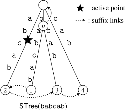
In other words, for every , we can update to in amortized time. Ukkonen’s algorithm maintains the active point in the suffix tree, which is the locus of the longest repeating suffix of the string. To maintain the active point efficiently, Ukkonen’s algorithm uses auxiliary data structures called suffix links: Each internal node of the suffix tree has a suffix link that points to the node , such that is the suffix of of length . See Fig. 1 for examples of a suffix tree and related notations.
Furthermore, based on Ukkonen’s algorithm, we can maintain suffix trees for a sliding window over in a total of time, using space proportional to the window size:
Theorem 2 ([17, 25, 33, 26]).
Using space, a suffix tree for a variable-width sliding window can be maintained in amortized time per one operation: either (1) appending a character to the right or (2) deleting the leftmost character from the window, where is the maximum width of the window. Additionally, the length of the longest repeating suffix of the window can be maintained with the same time complexity.
In other words, for every incremental pair of indices with , we can update to either or in amortized time. Later, we use the above algorithmic results as black boxes.
2.3 Weighted ancestor queries
For a node-weighted tree , where the weight of each non-root node is greater than the weight of its parent, a weighted ancestor query (WAQ) is defined as follows: given a node of the tree and an integer , the query returns the farthest (highest) ancestor of whose weight is at least . We denote by the returned node for weighted ancestor query on tree . The subscript will be omitted when clear from the context. In general, a WAQ on a tree of size can be answered in time, which is worst-case optimal with linear space. However, if the input is the suffix tree of some string of length , and the weight function is , as defined in the previous subsection, any WAQ can be answered in time after -time preprocessing [10].
3 Counting closed factors online
In this section, we propose an algorithm to count the distinct closed factors for a string given in an online manner. Since there may be distinct closed factors in a string of length [5, 31], enumerating them requires quadratic time in the worst case. However, for counting the closed factors, we can achieve subquadratic time even when the string is given in an online manner, as described below.
3.1 Changes in number of closed factors
First we consider the changes in the number of distinct closed factors when a character is appended. Let be the set of distinct closed factors occurring in . Let for . For convenience let .
Observation 1.
For any closed suffixes and of the same string, holds if .
Based on this observation, we count the distinct borders of closed factors instead of the closed factors themselves. We show the following:
Lemma 1.
For each with , holds if . Also, holds if .
Proof.
The latter case is obvious since implies that is a unique character in , making it the only new closed factor. In the following, we assume and denote and . It can be observed that for any new closed factor , is a unique suffix of and the longest border of repeats in . Equivalently, and hold. Additionally, implies . Thus , and hence by Observation 1. Conversely, for any suffix of satisfying , there exists exactly one closed suffix whose longest border is since is repeating in . Further, since , the closed suffix is longer than , and thus the closed suffix is unique in . Therefore, holds. ∎
We note that the upper bound of is already claimed in [31], however, the equality was not shown. By definition of and Lemma 1, the next corollary immediately follows:
Corollary 1.
The total number of distinct closed factors of is
where .
3.2 Online algorithm
By Theorem 1, we can compute in time online. Thus, by Corollary 1, our remaining task is to compute online, equivalently, to compute the sequence where for each . To compute the sequence, we use sliding suffix trees of Theorem 2. It is known that the starting position of is not smaller than that of . Namely, starting from , the sequence of factors of can be obtained by sliding-operations on that consists of (1) appending a character to the right or (2) deleting the leftmost character from the factor, where for each . Thus, by Theorem 2, we can obtain every in amortized time by appropriately applying sliding-operations to reach the windows for all with in order. Finally, we obtain the following:
Theorem 3.
For a string of length given in an online manner, we can count the distinct closed factors of in time using space where is the alphabet size.
4 Counting closed factors offline: shaving log factor
In this section, we assume that the alphabet is linearly sortable, allowing us to construct in time offline [16]. Our goal is to remove the factor from the complexity in Theorem 3, which arises from using dynamic predecessor dictionaries (e.g., AVL trees) at non-leaf nodes. To shave this logarithmic factor, we do not rely on such dynamic dictionaries. Instead, use a WAQ data structure constructed over .
Simulating sliding suffix tree in linear time.
The idea is to simulate the online algorithm from Section 3 using the suffix tree of the entire string . In algorithms underlying Theorem 1 and 2, the topology of suffix trees and the loci of the active points change step-by-step. The changes include (i) moving the active point, (ii) adding a node, an edge, or a suffix link, and (iii) removing a node, an edge, or a suffix link.
Our data structure consists of two suffix trees:
-
(1)
The suffix tree of enhanced with a WAQ data structure.
-
(2)
The suffix tree of the factor , which represents a sliding window.
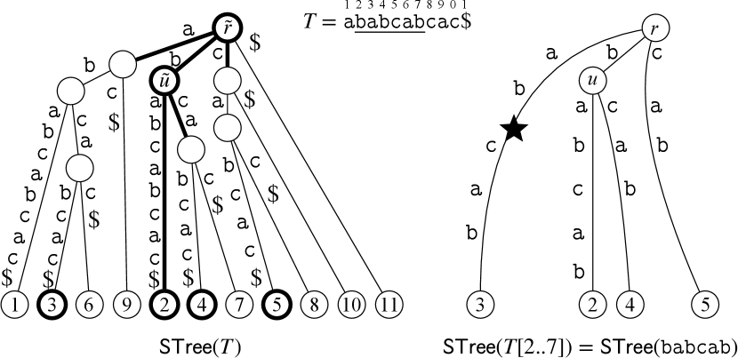
Note that includes the active point. All nodes and edges of are connected to their corresponding nodes and edges in . Specifically, an internal node of is connected to the node of where . Similarly, an edge of is connected to the edge of where the first characters of the edge-labels are the same. Such node and edge in always exist: An internal node implies that, for some distinct characters and , and occur in , and thus also in . Furthermore, a leaf of , representing suffix of , is connected to the leaf of representing the suffix of . Note that suffix links of do not connect to and are maintained within . See Fig. 2 for illustration.
We maintain the active point in as follows:
-
•
When the active point is on an edge and moves down, if the character on the edge following the active point matches the next character , the active point simply moves down. Otherwise, if the active point cannot move down, we create a new branching node at the locus and add a new leaf and edge . The new leaf and edge are connected to the corresponding edge and leaf of as the above discussion. The edge of can be found in constant time using a weighted ancestor query on .
-
•
Similarly, when the active point is a node and moves down, if represents , we query and check the resulting edge. The resulting edge of is already connected to an edge of the smaller suffix tree if and only if has an outgoing edge whose edge label starts with . If the active point can move down to the existing edge, we simply move it to the edge (via its corresponding edge in ). Otherwise, we create a new leaf and edge , connecting them to their corresponding leaf and edge of as described above.
In Ukkonen’s algorithm, a new node/edge is created only if the active point reaches it, so every node/edge creation can be simulated as described. Node/edge deletions are straightforward: we simply disconnect the node/edge from and remove them. Therefore, we can simulate the sliding suffix tree over in amortized time per sliding-operation. We have shown the next theorem:
Theorem 4.
Given an offline string over a linearly sortable alphabet, we can simulate a suffix tree for a sliding window in a total of time.
Corollary 2.
We can count the distinct closed factors in over a linearly sortable alphabet in time using space.
5 Enumerating closed factors offline
In this section, we discuss the enumeration of (distinct) closed factors in an offline string . We first consider The open-close-array of , which is the binary sequence of length where iff is closed [28]. Since an open-close-array can be computed in time, we can enumerate all the occurrences of closed factors of in time by constructing for all . We then map the occurrences to their corresponding loci on using constant-time WAQs times. Thus we have the following:
Proposition 1.
We can enumerate all the occurrences of closed factors of and the distinct closed factors of in time.
Next, we propose an alternative approach that can achieve subquadratic time when there are few closed factors to output. Using the algorithms described in Sections 3 and 4, we can enumerate the ending positions and the longest borders of distinct closed factors in time. For each such a border of a closed factor, we need to determine the starting position of the closed factor by finding the nearest occurrence of to the left. Such occurrences can be computed efficiently by utilizing range predecessor queries over the list of (the integer-labels of) the leaves of as follows: Let be a border of some closed factor where occurs exactly twice in . We first find the locus of in by a WAQ. Let be the nearest descendant of the locus, inclusive. Then, the leaves in the subtree rooted at represent the occurrences of in . Thus the nearest occurrence of to the left equals the predecessor value of within the leaves under . By applying Belazzougui and Puglisi’s range predecessor data structure [11], we obtain the following:
Proposition 2.
We can enumerate the distinct closed factors of in time where is the number of distinct closed factors in and is a fixed constant with .
6 Conclusions
In this paper, we proposed two algorithms for counting distinct closed factors of a string. The first algorithm runs in time using space for a string given in an online manner. The second algorithm runs in time and space for a static string over a linearly sortable alphabet. Additionally, we discussed how to enumerate the distinct closed factors, and showed a -time algorithm using open-close-arrays, as well as an -time algorithm that combines our counting algorithm with a range predecessor data structure. Since there can be distinct closed factors in a string [5, 31], the term can be superquadratic in the worst case. This leads to the following open question: For the enumerating problem, can we achieve time, which is linear in the output size?
References
- [1] Hayam Alamro, Mai Alzamel, Costas S. Iliopoulos, Solon P. Pissis, Wing-Kin Sung, and Steven Watts. Efficient identification of k-closed strings. Int. J. Found. Comput. Sci., 31(5):595–610, 2020.
- [2] Mai Alzamel, Costas S. Iliopoulos, W. F. Smyth, and Wing-Kin Sung. Off-line and on-line algorithms for closed string factorization. Theor. Comput. Sci., 792:12–19, 2019.
- [3] Golnaz Badkobeh, Hideo Bannai, Keisuke Goto, Tomohiro I, Costas S. Iliopoulos, Shunsuke Inenaga, Simon J. Puglisi, and Shiho Sugimoto. Closed factorization. In Proceedings of the Prague Stringology Conference 2014, Prague, Czech Republic, September 1-3, 2014, pages 162–168. Department of Theoretical Computer Science, Faculty of Information Technology, Czech Technical University in Prague, 2014.
- [4] Golnaz Badkobeh, Hideo Bannai, Keisuke Goto, Tomohiro I, Costas S. Iliopoulos, Shunsuke Inenaga, Simon J. Puglisi, and Shiho Sugimoto. Closed factorization. Discret. Appl. Math., 212:23–29, 2016.
- [5] Golnaz Badkobeh, Gabriele Fici, and Zsuzsanna Lipták. On the number of closed factors in a word. In Language and Automata Theory and Applications - 9th International Conference, LATA 2015, Nice, France, March 2-6, 2015, Proceedings, volume 8977 of Lecture Notes in Computer Science, pages 381–390. Springer, 2015.
- [6] Golnaz Badkobeh, Alessandro De Luca, Gabriele Fici, and Simon J. Puglisi. Maximal closed substrings. In String Processing and Information Retrieval - 29th International Symposium, SPIRE 2022, Concepción, Chile, November 8-10, 2022, Proceedings, volume 13617 of Lecture Notes in Computer Science, pages 16–23. Springer, 2022.
- [7] Golnaz Badkobeh, Alessandro De Luca, Gabriele Fici, and Simon J. Puglisi. Maximal closed substrings. CoRR, abs/2209.00271, 2022.
- [8] Hideo Bannai, Shunsuke Inenaga, Tomasz Kociumaka, Arnaud Lefebvre, Jakub Radoszewski, Wojciech Rytter, Shiho Sugimoto, and Tomasz Walen. Efficient algorithms for longest closed factor array. In String Processing and Information Retrieval - 22nd International Symposium, SPIRE 2015, London, UK, September 1-4, 2015, Proceedings, volume 9309 of Lecture Notes in Computer Science, pages 95–102. Springer, 2015.
- [9] Djamal Belazzougui, Manuel Cáceres, Travis Gagie, Pawel Gawrychowski, Juha Kärkkäinen, Gonzalo Navarro, Alberto Ordóñez Pereira, Simon J. Puglisi, and Yasuo Tabei. Block trees. J. Comput. Syst. Sci., 117:1–22, 2021.
- [10] Djamal Belazzougui, Dmitry Kosolobov, Simon J. Puglisi, and Rajeev Raman. Weighted ancestors in suffix trees revisited. In 32nd Annual Symposium on Combinatorial Pattern Matching, CPM 2021, July 5-7, 2021, Wrocław, Poland, volume 191 of LIPIcs, pages 8:1–8:15. Schloss Dagstuhl - Leibniz-Zentrum für Informatik, 2021.
- [11] Djamal Belazzougui and Simon J. Puglisi. Range predecessor and Lempel-Ziv parsing. In Proceedings of the Twenty-Seventh Annual ACM-SIAM Symposium on Discrete Algorithms, SODA 2016, Arlington, VA, USA, January 10-12, 2016, pages 2053–2071. SIAM, 2016.
- [12] Michelangelo Bucci, Aldo de Luca, and Alessandro De Luca. Rich and periodic-like words. In Developments in Language Theory, 13th International Conference, DLT 2009, Stuttgart, Germany, June 30 - July 3, 2009. Proceedings, volume 5583 of Lecture Notes in Computer Science, pages 145–155. Springer, 2009.
- [13] Arturo Carpi and Aldo de Luca. Periodic-like words, periodicity, and boxes. Acta Informatica, 37(8):597–618, 2001.
- [14] Maxime Crochemore, Lucian Ilie, and Wojciech Rytter. Repetitions in strings: Algorithms and combinatorics. Theor. Comput. Sci., 410(50):5227–5235, 2009.
- [15] Fabien Durand. A characterization of substitutive sequences using return words. Discret. Math., 179(1-3):89–101, 1998.
- [16] Martin Farach. Optimal suffix tree construction with large alphabets. In 38th Annual Symposium on Foundations of Computer Science, FOCS ’97, Miami Beach, Florida, USA, October 19-22, 1997, pages 137–143. IEEE Computer Society, 1997.
- [17] Edward R. Fiala and Daniel H. Greene. Data compression with finite windows. Commun. ACM, 32(4):490–505, 1989.
- [18] Gabriele Fici. A classification of trapezoidal words. In Proceedings 8th International Conference Words 2011, Prague, Czech Republic, 12-16th September 2011, volume 63 of EPTCS, pages 129–137, 2011.
- [19] Gabriele Fici. Open and closed words. Bulletin of EATCS, (123), 2017.
- [20] Zvi Galil and Joel I. Seiferas. Time-space-optimal string matching. J. Comput. Syst. Sci., 26(3):280–294, 1983.
- [21] Amy Glen, Jacques Justin, Steve Widmer, and Luca Q. Zamboni. Palindromic richness. Eur. J. Comb., 30(2):510–531, 2009.
- [22] Dominik Kempa and Nicola Prezza. At the roots of dictionary compression: string attractors. In Proceedings of the 50th Annual ACM SIGACT Symposium on Theory of Computing, STOC 2018, Los Angeles, CA, USA, June 25-29, 2018, pages 827–840. ACM, 2018.
- [23] Donald E. Knuth, James H. Morris Jr., and Vaughan R. Pratt. Fast pattern matching in strings. SIAM J. Comput., 6(2):323–350, 1977.
- [24] Tomasz Kociumaka, Gonzalo Navarro, and Francisco Olivares. Near-optimal search time in -optimal space, and vice versa. Algorithmica, 86(4):1031–1056, 2024.
- [25] N. Jesper Larsson. Extended application of suffix trees to data compression. In Proceedings of the 6th Data Compression Conference (DCC ’96), Snowbird, Utah, USA, March 31 - April 3, 1996, pages 190–199. IEEE Computer Society, 1996.
- [26] Laurentius Leonard, Shunsuke Inenaga, Hideo Bannai, and Takuya Mieno. Constant-time edge label and leaf pointer maintenance on sliding suffix trees. CoRR, abs/2307.01412, 2024.
- [27] Alessandro De Luca and Gabriele Fici. Open and closed prefixes of sturmian words. In Combinatorics on Words - 9th International Conference, WORDS 2013, Turku, Finland, September 16-20. Proceedings, volume 8079 of Lecture Notes in Computer Science, pages 132–142. Springer, 2013.
- [28] Alessandro De Luca, Gabriele Fici, and Luca Q. Zamboni. The sequence of open and closed prefixes of a Sturmian word. Adv. Appl. Math., 90:27–45, 2017.
- [29] Gonzalo Navarro. Indexing highly repetitive string collections, part I: repetitiveness measures. ACM Comput. Surv., 54(2):29:1–29:31, 2022.
- [30] Gonzalo Navarro. Indexing highly repetitive string collections, part II: compressed indexes. ACM Comput. Surv., 54(2):26:1–26:32, 2022.
- [31] Olga G. Parshina and Svetlana Puzynina. Finite and infinite closed-rich words. Theor. Comput. Sci., 984:114315, 2024.
- [32] Olga G. Parshina and Luca Q. Zamboni. Open and closed factors in arnoux-rauzy words. Adv. Appl. Math., 107:22–31, 2019.
- [33] Martin Senft. Suffix tree for a sliding window: An overview. In 14th Annual Conference of Doctoral Students - WDS 2005, pages 41–46. Matfyzpress, 2005.
- [34] W. F. Smyth. Computing regularities in strings: A survey. Eur. J. Comb., 34(1):3–14, 2013.
- [35] Wataru Sumiyoshi, Takuya Mieno, and Shunsuke Inenaga. Faster and simpler online/sliding rightmost lempel-ziv factorizations. In String Processing and Information Retrieval - 31th International Symposium, SPIRE 2024, volume 14899 of Lecture Notes in Computer Science, pages 321–335. Springer, 2024.
- [36] Esko Ukkonen. On-line construction of suffix trees. Algorithmica, 14(3):249–260, 1995.
- [37] Laurent Vuillon. A characterization of sturmian words by return words. Eur. J. Comb., 22(2):263–275, 2001.
- [38] Peter Weiner. Linear pattern matching algorithms. In 14th Annual Symposium on Switching and Automata Theory, Iowa City, Iowa, USA, October 15-17, 1973, pages 1–11. IEEE Computer Society, 1973.