Online differentially private inference in stochastic gradient descent
Abstract
We propose a general privacy-preserving optimization-based framework for real-time environments without requiring trusted data curators. In particular, we introduce a noisy stochastic gradient descent algorithm for online statistical inference with streaming data under local differential privacy constraints. Unlike existing methods that either disregard privacy protection or require full access to the entire dataset, our proposed algorithm provides rigorous local privacy guarantees for individual-level data. It operates as a one-pass algorithm without re-accessing the historical data, thereby significantly reducing both time and space complexity. We also introduce online private statistical inference by conducting two construction procedures of valid private confidence intervals. We formally establish the convergence rates for the proposed estimators and present a functional central limit theorem to show the averaged solution path of these estimators weakly converges to a rescaled Brownian motion, providing a theoretical foundation for our online inference tool. Numerical simulation experiments demonstrate the finite-sample performance of our proposed procedure, underscoring its efficacy and reliability. Furthermore, we illustrate our method with an analysis of two datasets: the ride-sharing data and the US insurance data, showcasing its practical utility.
1Yunnan Key Laboratory of Statistical Modeling and Data Analysis, Yunnan University
2Department of Mathematical and Statistical Sciences, University of Alberta
3Department of Statistics and Data Science, Washington University in St. Louis
Keywords: Confidence interval; Local differential privacy; Privacy budget; Stochastic gradient descent.
1 Introduction
Online learning involves methods and algorithms designed for making timely inferences and predictions in a real-time environment, where data are collected sequentially rather than being static as in traditional batch learning. By not requiring the simultaneous use of the entire sample pool, online learning alleviates both storage and computation pressures. To date, various statistical methods and algorithms for online estimation and inference have been proposed, including aggregated estimating equations (Lin and Xi, 2011), cumulative estimating equation (Schifano et al., 2016), renewable estimator (Luo and Song, 2020), and stochastic gradient descent (SGD) (Robbins and Monro, 1951; Polyak and Juditsky, 1992; Chen et al., 2020). Alongside online learning, another crucial consideration is the preservation of privacy, especially with the growing availability of streaming data. For example, financial institutions, such as banks and credit card companies, often leverage customer-level data for fraud detection and personalized service offerings, which need to continuously update and refine their models in real-time as new transaction data are collected. This aids not only in monitoring transactions to detect unusual activities but also in designing targeted financial products and promotions (e.g., offering personalized loan rates or credit card rewards based on individual spending patterns); see Maniar et al. (2021); Davidow et al. (2023). However, individual customer data are usually sensitive and irreplaceable, and it is of great importance to prevent the leak of personal information to maintain customer trust and confidence, as well as to help businesses avoid financial losses and reputational damage (Hu et al., 2022; Fainmesser et al., 2023).
In response to the increasing demand for data privacy protection, differential privacy (DP) has emerged as a widely adopted concept (Dwork et al., 2006). It has been successfully applied in numerous fields, including healthcare, financial services, retail, and e-commerce (Dankar and El Emam, 2013; Zhong, 2019; Wang and Tsai, 2022). DP procedures ensure that an adversary cannot determine whether a particular subject is included in the dataset with high probability, thereby providing robust protection for personal information. In the literature, two main models have emerged for DP: the central model, where a trusted third party collects and analyzes data before releasing privatized results, and the local model, where data is randomized before sharing. Several works have focused on designing private algorithms to guarantee DP under the trusted central server setting across various applications, including, but not limited to, machine learning, synthetic data generation, and transfer learning; see Karwa and Slavković (2016); Ponomareva et al. (2023); Li et al. (2024). A significant limitation of the standard central model is the assumption of a trusted data curator with access to the entire dataset. However, in scenarios such as smartphone usage, users may not fully trust the server and prefer not to have their personal information directly stored or updated on any remote central server. In contrast to the central DP, user-level local differential privacy (LDP) does not rely on a trusted data collector, placing the privacy barrier closer to the users, which has seen adoption in practice by several companies that analyze sensitive user data, including Apple (Tang et al., 2017), Google (Erlingsson et al., 2014), and Microsoft (Ding et al., 2017). Recently, there has been growing interest in studying LDP from a statistical perspective, including density estimation (Sart, 2023), mean and median estimation (Duchi et al., 2018), nonparametric estimation problems (Rohde and Steinberger, 2020), and change-point detection (Berrett and Yu, 2021).
The aforementioned methods mainly address the inherent trade-off between privacy protection and efficient statistical inference, focusing on identifying what optimal privacy-preserving mechanisms may look like. The literature on private inference, particularly in quantifying the uncertainty of private estimators, is relatively limited even in offline settings and has recently gained attention in computer science (Karwa and Vadhan, 2018; Wang et al., 2019; Chadha et al., 2021). This issue has also been studied in the statistical literature. Sheffet (2017) provided finite-sample analyses of conservative inference for confidence intervals regarding the coefficients from the least-squares regression. Barrientos et al. (2019) presented algorithms for comparing the sign and significance level of privately computed regression coefficients that satisfy DP. Avella-Medina (2021) introduced the M-estimator approach to conduct DP statistical inference using smooth sensitivity. Alabi and Vadhan (2023) proposed DP hypothesis tests for the multivariate linear regression model. Avella-Medina et al. (2023) investigated optimization-based approaches for Gaussian differentially private M-estimators. Zhao et al. (2024) extended this to objective functions without local strong convexity and smoothness assumptions. Zhang et al. (2024) considered estimation and inference problems in the federated learning setting under DP. Despite these efforts, a significant gap remains in developing a statistically sound approach for conducting statistical inference, such as constructing confidence intervals based on private estimators, particularly in the online setting, where theoretical results for statistical inference are largely lacking. Recently, Liu et al. (2023) proposed a self-normalizing approach to obtain confidence intervals for population quantiles with privacy concerns. However, this method is specifically tailored to population quantiles.
In this paper, we introduce a rigorous LDP framework for online estimation and inference in optimization-based regression problems with streaming data, addressing the challenge of constructing valid confidence intervals for online private inference. Specifically, we propose a fully online, locally private framework for real-time estimation and inference without requiring trusted data collectors. To the best of our knowledge, this is the first time in the literature on online inference problems where the issue of privacy is systematically investigated. The main contributions of this paper are summarized as follows:
-
1.
To eliminate the need for trusted data collectors, we design a local differential privacy stochastic gradient descent algorithm (LDP-SGD) for streaming data that requires only one pass over the data. Unlike prior works, our algorithm provides rigorous individual-level data privacy protection in an online manner. Meanwhile, we propose two online private statistical inference procedures. One is to conduct a private plug-in estimator of the asymptotic covariance matrix. The other is the random scaling procedure, bypasses direct estimation of the asymptotic variance by constructing an asymptotically pivotal statistic for valid private inference in real time.
-
2.
From a theoretical standpoint, we establish the convergence rates of the proposed online private estimators. In addition, we prove a functional central limit theorem to capture the asymptotic behavior of the whole LDP-SGD path, thereby providing an asymptotically pivotal statistic for valid private inference. These results lay a solid foundation for real-time private decision-making, supported by theoretical guarantees.
-
3.
We conduct numerical experiments with simulated data to evaluate the performance of the proposed procedure in various settings, including varying cumulative sample size, different privacy budgets, and various models. Our findings indicate that the proposed procedure is computationally efficient, provides robust privacy guarantees, and significantly reduces data storage costs, all while maintaining high accuracy in estimation and inference. In addition, we apply the proposed method to the the ride-sharing data and the US insurance data to demonstrate how the method can be useful in practice.
The rest of this paper is organized as follows. In Section 2.1, we introduce the key properties of DP. Section 2.2 outlines the problem formulation. In Section 3, we propose our LDP-SGD algorithm and provide its convergence rates. In Section 4, we establish a functional central limit theorem and introduce two online private inference methods: the private plug-in estimator and the random scaling method to construct asymptotically valid private confidence intervals. We evaluate the performance of the proposed procedure through simulation studies in Section 5. In Section 6, we apply the proposed method on two real-world datasets: the Ride-Sharing Data and the US Insurance Data. Ride-sharing data provides fare-related information over time, enabling analysis of market pricing dynamics in the ride-sharing industry. The US Insurance Data includes detailed personal and family information for one million clients, along with their associated insurance fees, offering valuable insights into insurance fee prediction. Discussions are provided in Section 7. Some basic concepts of DP, the detailed description of private batch-means estimator, additional numerical results, and technical details are included in the Supplementary Material.
2 Preliminaries
In this section, we provide some preliminaries. To facilitate understanding, we first introduce the notations used throughout this paper. Let denote convergence in distribution. For a -vector , for . Define as the eigenvalues of a matrix . Specifically, the largest and smallest eigenvalues are denoted by and , respectively. We use to denote the matrix operator norm of and to represent the element-wise -norm of . For a square positive semi-definite matrix , we denote its trace by . For any two symmetric matrices and of the same dimension, means that is a positive semi-definite matrix, while means that is a positive semi-definite matrix. Let and be two sequences of positive numbers. Denote if there exists a positive constant such that for all , and if there exist positive constants , such that for all .
2.1 Some basic properties of differential privacy
In this subsection, we only focus on some useful properties of DP, LDP, and Gaussian differential privacy (GDP), while more details about GDP-related concepts are provided in the Supplementary Material. Notice that a variety of basic algorithms can be made private by simply adding a properly scaled noise in the output. The scale of noise is characterized by the sensitivity of the algorithm. The formal definition is presented as follows:
Definition 1 (Global sensitivity).
For any (non-private) statistics of the data set , the global sensitivity of is the (possibly infinite) number
where the supremum is taken over all pairs of data sets and that differ by one entry or datum.
We then introduce the following mechanism to construct GDP estimators. Although only the univariate case was stated in Theorem 1 of Dong et al. (2022), its extension to general case can be obtained in the following proposition.
Proposition 1 (Gaussian mechanism, Dong et al. (2022)).
Define the Gaussian mechanism that operates on a statistic as , where is a standard normal -dimensional random vector and . Then, is -GDP.
The post-processing and parallel composition properties are key aspects of DP, enabling the design of complex DP algorithms by combining simpler ones. Such properties are crucial in the algorithmic designs presented in later sections.
Proposition 2 (Post-processing property, Dong et al. (2022)).
Let be an -GDP algorithm, and be an arbitrary randomized algorithm which takes as input, then is also -GDP.
Proposition 3 (Parallel composition, Smith et al. (2022)).
Let a sequence of mechanisms each be -GDP, . Let be disjoint subsets of data. Define as the output of the mechanism , and the sequential output of the mechanism is defined as for . Then the output of the last mechanism is -GDP.
Since we will use a noisy version of the matrix to construct an asymptotic covariance matrix in a later section, we introduce the Matrix Gaussian mechanism. An intuitive approach to generating a differentially private matrix is to add independent and identically distributed (i.i.d.) noise to each individual component, as described below.
Proposition 4 (Matrix Gaussian mechanism, Avella-Medina et al. (2023)).
Let be a data matrix such that each row vector satisfies . Define the matrix Gaussian mechanism that operates on a statistic as , where and is a symmetric random matrix whose upper-triangular elements, including the diagonal, are i.i.d. draws from . Then, is -GDP.
2.2 Problem formulation
Consider , where observations, denoted by with arrive sequentially. We assume these pairs of observations as i.i.d. copies of with and from a common cumulative distribution . Our goal is to estimate a population parameter of interest , which can be formulated as the solution to the following optimization problem:
| (2.1) |
where is some convex loss function with respect to , is a random variable from the distribution , and is the population loss function.
In the offline setting, where the entire dataset is readily accessible, traditional deterministic optimization methods are commonly used to estimate the parameter under the empirical distribution induced by the observed data. However, for applications involving online data, where each sample arrives sequentially, storing all the data can be costly and inefficient. To address these challenges, the SGD algorithm (Robbins and Monro, 1951) is often used, especially for online learning, as it requires only one pass over the data. Starting from an initial point , the SGD algorithm recursively updates the estimate upon the arrival of each data point , , with the following update rule:
| (2.2) |
where denotes the stochastic gradient of with respect to the first argument , i.e., and is the step size at the th step. As suggested by Ruppert (1988) and Polyak and Juditsky (1992), we note that under some conditions, the averaging estimate has the asymptotic normality
where , is the Hessian matrix of at , and is the covariance matrix of , given by .
A significant limitation of traditional SGD is its vulnerability to privacy breaches, arising from the extensive data and gradient queries made at each iteration. In this paper, our work focuses primarily on settings where trusted data collectors are not required under the constraints of LDP. In such settings, each individual is required to locally apply a DP mechanism to their data before transmitting the perturbed data to the server. In particular, we introduce an LDP-SGD algorithm designed to fit the model in (2.1) and accommodate timely online private statistical inference for , thereby providing rigorous individual-level data privacy protection while reducing both time and space complexity.
3 Methodology
In this subsection, we introduce an LDP estimator using noisy SGD algorithms within the framework of streaming data. The heightened risk of privacy leakage arises from the numerous data and gradient queries inherent in the SGD algorithm. To facilitate our work, we impose a restriction on the class of estimators and enforce the following uniform boundedness condition.
Condition 1.
The gradient of the loss function satisfies
for some positive constant .
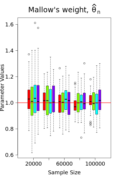
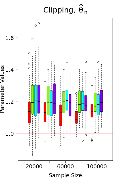
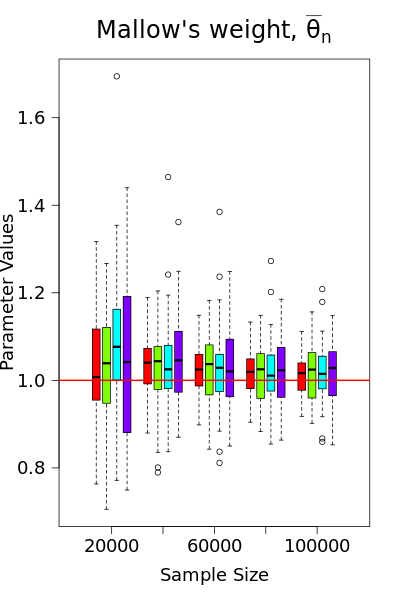
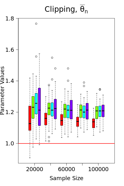
Condition 1 is satisfied by using either Mallow’s weights (as discussed in Examples 1-3) or gradient clipping. However, as demonstrated in Song et al. (2021); Avella-Medina et al. (2023), gradient clipping is not ideal from a statistical standpoint, as it may result in inconsistent estimators. In Figure 1, we compare the performance of gradient clipping and Mallow’s weights using simulated logistic regression data. The results show that the parameter estimates from gradient clipping exhibit bias that does not shrink toward zero with the sample size, further underscoring our preference for Mallow’s weights, alongside the assumption of a bounded gradient. Meanwhile, Condition 1 implies that the loss function has a known bound on the gradient , which ensures that is an upper bound for the global sensitivity of . At the th iteration with observed data point , , we consider the following locally private SGD estimator with the noisy version of the iterates (2.2)
| (2.3) |
where the final estimate is the averaging estimate denoted by and is a sequence of i.i.d. standard -dimensional Gaussian random vectors. Unlike the standard SGD algorithm, the locally private SGD algorithm introduces calibrated noise to the gradient computations at each step of the model parameter update process, ensuring rigorous privacy protection. In particular, taking in the iterates (2.3) recovers the standard SGD algorithm in (2.2). We call the proposed iterates in (2.3) as the LDP-SGD algorithm. The following proposition shows that our proposed LDP-SGD algorithm is -GDP.
Proposition 5.
Given an initial estimate , consider the iterates defined in (2.3). Then the final output is -GDP.
From (2.3), each individual has different privacy budgets , A special case arises when the proposed estimator reduces to -GDP with , thereby not considering different privacy budgets for each individual. The techniques needed to handle the cases of varing are the same as for the case of the common . For simplicity, we assume that for each individual.
Condition 2.
Assume that the objective function is differentiable, -smooth, and -strongly convex, in the sense
Strong convexity and smoothness are standard conditions for the convergence analysis of (stochastic) gradient optimization methods. Similar conditions can be found in Vaswani et al. (2022); Zhu et al. (2023). Due to space limitations, several useful properties of strongly convex and smooth functions are provided in Lemma S1 of the Supplementary Material. As stated in Lemma S1, the strong convexity and smoothness of imply that and , respectively.
Condition 3.
Let denote the gradient noise. There exists some positive constant such that the conditional covariance of has an expansion around , satisfies
where is the -algebra generated by and is the error sequence. In addition, the fourth conditional moment of is bounded by
for some positive constant
Condition 3 is a mild requirement on the loss function. As shown in Lemma 3.1 of Chen et al. (2020), Condition 3 holds if the Hessian matrix of is bounded by some random function with a bounded fourth moment. Examples that satisfy this condition include the robust estimation methods for commonly used linear and logistic regressions. With the aforementioned assumptions, we now present the following error bounds on the private SGD iterates.
Theorem 1.
Theorem 1 provides simplified bounds on the conditional moments of , including the first, second, and fourth moments. These results characterize the convergence rate of the last-step estimator . To illustrate the applicability of our proposed algorithm, we provide several examples below. Our framework, as it turns out, accommodates a wide range of important statistical models.
Example 1 (Linear Regression).
Let , be a sequence of i.i.d. copies from with and , satisfying , where is the random noise. The loss function can be chosen as , where is the Huber loss with truncated parameter and downweights outlying covariates. With this construction, it is straightforward to verify that the global sensitivity of is . Letting , our proposed LDP-SGD updates for , as defined in (2.3) is given by:
where is the indicator function.
Example 2 (Logistic Regression).
An important data science problem is logistic regression for binary classification problems. Specifically, let , be a sequence of i.i.d. copies from with and , satisfying . Taking Mallow’s weighted version of the usual cross-entropy loss as , where is defined in the previous example. By this construction, we can easily verify that the global sensitivity of is . Setting , our proposed LDP-SGD updates for , as defined in (2.3) is given by:
Example 3 (Robust Expectile Regression).
As an important extension of linear regression, robust expectile regression allows the regression coefficients to vary across different values of location parameter , and thereby offers insights into the entire conditional distribution of given ; see Man et al. (2024). Specifically, given a location parameter , let , be a sequence of i.i.d. copies from , satisfying . The loss function can be chosen as , where is the Huber loss with truncated parameter . With this construction, it is straightforward to verify that the global sensitivity of is . Taking , our proposed LDP-SGD updates for , as defined in (2.3) is given by:
4 Online private inference
In this subsection, we introduce two online inference methods, distinguished by the availability of second-order information from the loss function. One is the online private plug-in approach that directly uses the Hessian information and the other is the random scaling that utilizes only the information from the path of our proposed LDP-SGD iteration in (2.3). In addition to these two methods, we also consider a private batch-means estimator that utilizes the iterations generated by the LDP-SGD algorithm to estimate the asymptotic covariance. The detailed construction of this estimator, along with a comparative discussion of its theoretical properties relative to the above two methods, is provided in the Supplementary Material.
To elucidate these methods, we first examine the asymptotic behavior of the entire LDP-SGD path rather than its simple average . Specifically, we present the functional central limit theorem, which shows that the standardized partial-sum process converges in distribution to a rescaled Brownian motion.
Theorem 2 (Functional CLT).
Consider LDP-SGD iterates in (2.3) with step-size for some constant and . Then, under Conditions 1-3, the following random function weakly converges to a scaled Brownian motion, i.e.,
as , where , , is the -dimensional vector of the independent standard Wiener processes on , and the symbol stands for the weak convergence.
The result derived from this theorem is stronger than the asymptotic normality of the proposed private estimator under the stated assumptions. In particular, by applying the continuous mapping theorem to Theorem 2, we are able to directly establish the following corollary.
Corollary 1.
Under the conditions of Theorem 2, the averaging estimator satisfies , where , and .
In contrast to the covariance matrix of the non-private estimator in (2.2), the additional term in the covariance matrix of Corollary 1 represents the “cost of privacy” for our proposed LDP-SGD algorithm.
4.1 Private plug-in estimator
In the previous subsection, we present the asymptotic distribution of the proposed LDP-SGD estimator in Corollary 1. For the purpose of conducting statistical inference of , a consist estimator of the limiting covariance matrix from Corollary 1 is required. An intuitive way to constructing confidence intervals for is to estimate each component of the sandwich formula separately. Without privacy constraints, the estimators for and are given by:
as long as the information of is available. Notice that each summand in both and involves different . This allows computations to be carried out in an online manner without the need to store the entire dataset. The consistency of the corresponding non-private plug-in estimator is also established and provided in the Lemma S8 of the Supplementary Material.
However, in the DP setting, direct application of this plug-in construction is not feasible, as neither nor is differentially private. To overcome this limitation, we propose constructing DP versions of these matrices using the Matrix Gaussian mechanism, as outlined in Proposition 4. This requires the Hessian to have a specific factorization structure that facilitates the effective application of Proposition 4. Moreover, we assume that the spectral norm of the Hessian is uniformly bounded, as stated below.
Condition 4.
The Hessian is positive definite for all with the form , where and .
We are now ready to present our DP counterparts of and , which appear in the plug-in estimator. Consider the following private estimators:
where and are i.i.d. symmetric random matrices whose upper-triangular elements, including the diagonals, are i.i.d. standard normal. However, the DP matrices and can potentially be negative definite. To address this concern, we apply a truncation procedure to the eigenvalues of the matrices. Specifically, we first perform spectral decompositions: and , where and are orthogonal matrices. Given fixed threshold parameters and , we define the truncated estimators as and , where the diagonal elements are thresholded as and for . In other words, eigenvalues smaller than or are truncated to ensure numerical stability and positive semi-definiteness. The DP sandwich estimator can then be constructed as follows:
| (2.4) |
To establish consistency of our proposed private plug-in estimator , we need the following additional smoothness assumption regarding the Hessian, similar to those found in the literature (Chen et al., 2020, 2024).
Condition 5.
Assume that for all , the following holds:
where and are some postive constants. Furthermore, assume that
Theorem 3 (Error rate of the private plug-in estimator).
Theorem 3 establishes the consistency of the proposed private plug-in estimator . Consequently, we can consider the following -GDP -confidence interval for , :
where and is the ()-quantile of the standard normal distribution. In particular, we have the following corollary, which demonstrates that is an asymptotically exact confidence interval.
Corollary 2.
Under the conditions of Theorem 3, when is fixed and , we have
4.2 Random scaling
Despite the simplicity of the private plug-in approach, the proposed estimator incurs additional computational and storage cost, primarily because it requires extra function-value queries to construct . To mitigate this issue, we propose the random scaling inference procedure, which avoids the direct estimation of the asymptotic variance. Instead, the procedure studentizes using a matrix derived from iterations along the LDP-SGD path. Specifically, with Theorem 2, we observe that . Consequently, eliminates the dependence on . To remove the dependence on the unknown scale , we studentize via
This results in the statistic being asymptotically pivotal, with a distribution that is free of any unknown nuisance parameters. This conclusion is supported by the following corollary, which directly follows from Theorem 2 and the continuous mapping theorem. Thus, the proof of this corollary is omitted.
Corollary 3.
This corollary implies that can be used to construct valid asymptotic confidence intervals. From Corollary 3, we know that the -statistic , , is asymptotically pivotal and converges to the following pivotal limiting distribution
| (2.5) |
where . Notice that the random matrix can be updated in an online fashion, thereby enabling the construction of confidence intervals. Specifically,
where and can both be updated recursively. Once and are obtained, the asymptotic confidence interval for the th element of can be constructed as follows:
Corollary 4.
5 Simulation studies
In this section, we perform simulations to examine the finite-sample performance of the proposed algorithms, focusing on the coverage probabilities and lengths of confidence intervals. The methods under evaluation include the private plug-in (PPI), private batch-means (PBM), and private random scaling (PRS). As a benchmark, we also compute the non-private counterpart with plug-in (PI), batch-means (BM), and random scaling (RS). Due to space limitations, we only present the empirical performance of proposed algorithms under linear regression in our main manuscript. The results for logistic and robust expectile regressions are provided in the Supplementary Material.
In this simulation, we randomly generate a sequence of samples from the linear regression: , where the random noise is i.i.d. from and denotes the covariates, with following a multivariate normal distribution with two types of structure, identity covariance and correlated covariance . We consider a total sample size of arriving sequentially. For this model, the true coefficient is a ()-dimensional vector that includes the intercept term . The corresponding loss function and its gradient sensitivity are outlined in Example 1 with a step size decay rate of . For the identity covariance matrix, we vary the parameter dimensions across different privacy budgets . A smaller privacy budget corresponds to stronger privacy protection. In addition, we set the truncation parameter as used in the Huber loss and choose for the batch-means estimators, as suggested by Chen et al. (2020). This choice aligns with the optimal order when . Specifically, we set in our implementation. Owing to space constraints, this section reports only the results for . The corresponding results for and are available in the Supplementary Material. For the correlated covariance matrix, we only present results for , as similar patterns are observed in higher dimensions, as with the identity covariance matrix case.
The performance of each method is assessed using two criteria: the average empirical coverage probability of the 95% confidence interval (CP), and the average length of the 95% confidence interval (AL). Specifically. let CIj denote a two-side 95% confidence interval for , . We then calculate these two criteria across coefficients as below:
where and represent the empirical rate and the average length of the confidence intervals over all replications, respectively. All simulation results are based on 200 replications, with both the averages and standard errors recorded.
Figure 2 displays the trajectories of each component of the proposed LDP-SGD estimator with and along with three private confidence intervals for linear regression. As expected, the length of the confidence intervals decreases as increases. In the early iterations, both the estimators and confidence intervals are unstable, with noticeable fluctuations. The PRS method produces wider confidence intervals compared to PPI and PBM, indicating that PRS is more conservative than the other two methods. Additionally, the confidence interval widths for PPI and PBM are approximately equal. This observation aligns with findings from previous studies, such as those by Li et al. (2022) and Lee et al. (2022).
We also present the empirical performance of our proposed methods under varying total sample sizes, as detailed in Table 1. A key observation is that the performance of the proposed methods aligns more closely with their non-private counterparts as the privacy budget increases. The coverage probabilities for all three methods approach the desired level as the cumulative sample size or privacy budget increases, while the lengths of the confidence intervals decrease. Among these, the PRS method exhibits more robust performance across various settings and privacy budgets, albeit with slightly wider confidence intervals than the other two. Such a wider average length could potentially account for the improvement in the average coverage rates. In contrast, the PBM method exhibits relatively lower coverage compared to the PPI and PRS methods, consistent with theoretical results indicating that PBM converges more slowly than PPI. Under privacy-preserving conditions, all three methods result in lower coverage probabilities and wider confidence intervals compared to non-private version. This effect becomes more pronounced with smaller privacy budgets, illustrating the trade-off between maintaining privacy and achieving statistical accuracy. The corresponding results for and are provided in the Supplementary Material, demonstrating similar patterns.
meik 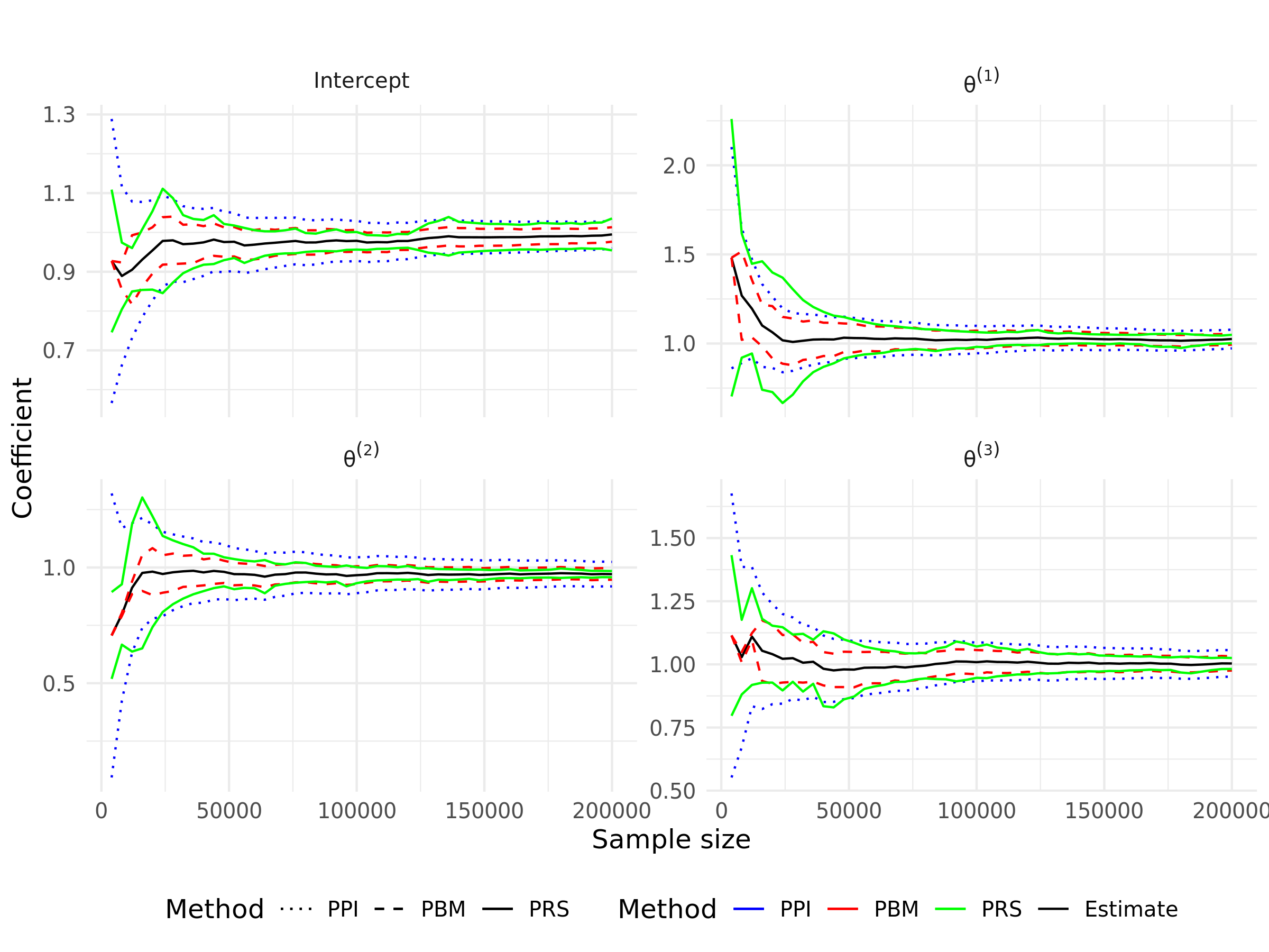
| Non-private | |||||
|---|---|---|---|---|---|
| PI: CP | 93.75 (3.66) | 92.50 (4.83) | 93.50 (3.54) | 92.75 (3.97) | 94.13 (3.09) |
| PI: AL | 1.08 (0.20) | 0.76 (0.14) | 0.62 (0.11) | 0.54 (0.10) | 0.48 (0.09) |
| BM: CP | 88.88 (2.01) | 90.75 (1.55) | 93.25 (2.50) | 93.13 (1.55) | 92.75 (1.26) |
| BM: AL | 1.01 (0.02) | 0.74 (0.01) | 0.62 (0.01) | 0.54 (0.01) | 0.48 (0.01) |
| RS: CP | 95.13 (1.38) | 94.00 (1.47) | 95.75 (0.50) | 95.13 (0.75) | 95.50 (1.22) |
| RS: AL | 1.47 (0.02) | 1.03 (0.02) | 0.84 (0.02) | 0.73 (0.03) | 0.64 (0.02) |
| PPI: CP | 91.38 (3.82) | 93.50 (4.30) | 92.13 (5.34) | 93.75 (3.18) | 93.25 (4.50) |
| PPI: AL | 11.49 (0.38) | 7.68 (0.19) | 6.10 (0.13) | 5.19 (0.10) | 4.60 (0.07) |
| PBM: CP | 85.38 (1.60) | 92.00 (1.41) | 91.63 (2.93) | 93.25 (2.02) | 92.88 (2.93) |
| PBM: AL | 11.09 (2.28) | 7.83 (1.57) | 6.49 (1.29) | 5.49 (1.05) | 4.77 (0.90) |
| PRS: CP | 94.38 (1.93) | 95.75 (0.29) | 94.88 (1.44) | 95.38 (2.32) | 95.50 (1.08) |
| PRS: AL | 16.01 (3.31) | 10.96 (2.21) | 8.64 (1.78) | 7.21 (1.28) | 6.50 (1.15) |
| PPI: CP | 90.75 (6.25) | 90.50 (4.88) | 91.25 (4.29) | 92.63 (3.42) | 92.13 (4.27) |
| PPI: AL | 4.99 (0.07) | 3.45 (0.08) | 2.81 (0.10) | 2.42 (0.10) | 2.16 (0.10) |
| PBM: CP | 84.63 (2.78) | 87.88 (2.63) | 89.75 (1.31) | 90.25 (1.00) | 90.88 (2.10) |
| PBM: AL | 4.70 (0.08) | 3.42 (0.06) | 2.87 (0.05) | 2.47 (0.04) | 2.15 (0.04) |
| PRS: CP | 92.75 (3.50) | 92.50 (1.78) | 93.50 (1.58) | 94.00 (1.62) | 94.88 (1.61) |
| PRS: AL | 6.77 (0.11) | 4.82 (0.09) | 3.94 (0.08) | 3.30 (0.06) | 2.93 (0.05) |
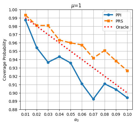
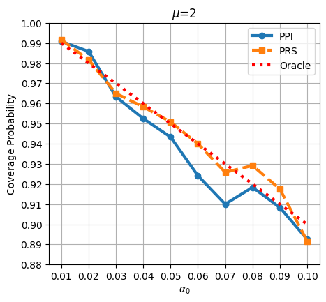
To further evaluate the coverage properties of PPI and PRS, we vary the significance level and compute the corresponding asymptotic confidence intervals, alongside the empirical coverage probabilities. Specifically, is varied from to in increments of . The analysis is carried out for a linear regression model with dimension and sample size , under two different privacy budgets . The results are presented in Figure 3. For , the PRS method exhibits a more conservative coverage probability, slightly surpassing the oracle coverage level, indicating minor over-coverage. In contrast, PPI tends to under-cover with its narrower confidence intervals. As the privacy budget increases to , both PRS and PPI coverage probabilities shift closer to the oracle curve.
6 Applications
In this section, we illustrate the effectiveness of the proposed method by analyzing two real-world datasets: the Ride-sharing data and the US insurance data.
6.1 Ride-sharing Data
In this subsection, we apply the proposed LDP-SGD algorithm to the Ride-sharing dataset, which contains synthetic data from a ride-sharing platform. The dataset spans from January 2024 to October 2024 and includes detailed records of rides, users, drivers, vehicles, and ratings. It offers valuable insights into driver performance and fare prediction over time. The dataset is publicly available at https://www.kaggle.com/datasets/adnananam/ride-sharing-platform-data, comprising 50,000 ride records and 3,000 profiles of drivers and vehicles. For preprocessing, we concatenate driver and vehicle information with each corresponding ride. We then select the following features as potential predictors for fare estimation: ride distance, driver rating, total number of rides completed by the driver, vehicle production year, vehicle capacity, and ride duration. After concatenation, the dataset is standardized by subtracting the mean and dividing by the standard deviation for each column. The resulting data is then used as input to the LDP-SGD algorithm with weighted Huber loss defined in Example 1, which is run with a privacy budget of and a step size decay rate of .
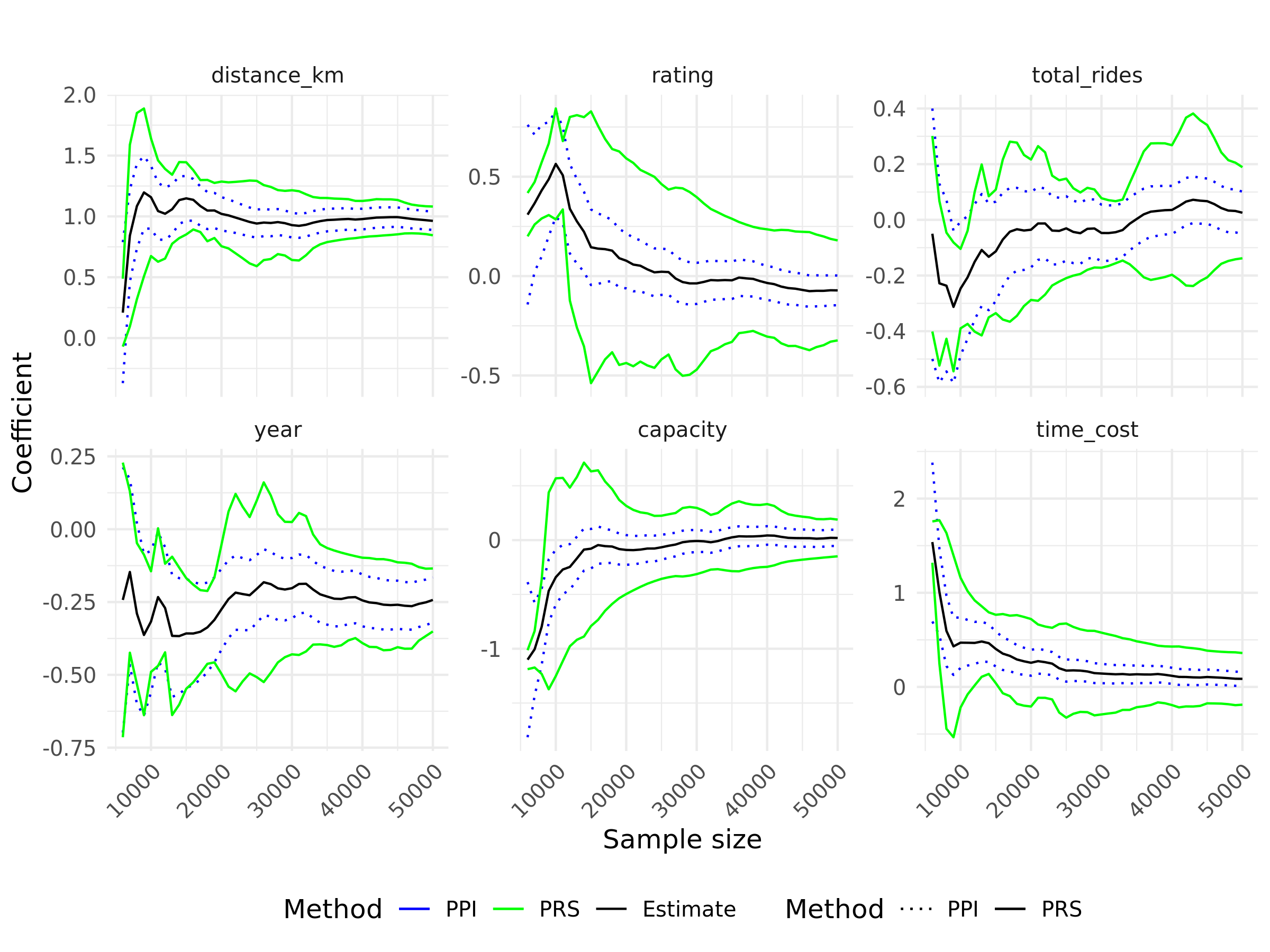
The results of this analysis are presented in Figure 4. As the sample size increases, the coefficients gradually stabilize. Specifically, the coefficients for ’distance’ and ’time cost’ converge to positive values, with both the PPI and PRS confidence intervals entirely above zero. This suggests a significant positive impact of these factors on fare amount, aligning with intuitive expectations, as longer distances and extended journey times are naturally associated with higher costs. In contrast, the coefficients for ’rating’ and ’total rides’ converge toward values near zero, with their confidence intervals including zero, indicating that driver-related attributes do not meaningfully affect fare pricing. Similarly, the coefficients for ’year’ and ’capacity’ also converge to values close to zero, with their confidence intervals encompassing zero, suggesting that vehicle-related factors have no significant influence on the fare amount. Overall, the analysis shows that only distance and time cost significantly impact fare pricing, while driver and vehicle characteristics have negligible effects. This is likely because ride fares are primarily driven by distance, duration, and demand fluctuations, which outweigh the influence of individual driver and vehicle attributes.
6.2 US insurance Data
In this subsection, we conduct a analysis on the Insurance dataset, which aims to predict health insurance premiums in the United States. The dataset, based on synthetic data, captures a variety of factors that influence medical costs and premiums. It includes the following variables on the insurance customers: age, gender, body mass index (BMI), number of children, smoking status, region, medical history, exercise frequency, occupation, and type of insurance plan. The full list of variables is presented in Table 2. This dataset was generated using a script that randomly sampled 1,000,000 records, ensuring a comprehensive representation of the insured population in the US. Publicly available at https://www.kaggle.com/datasets/sridharstreaks/insurance-data-for-machine-learning/data, it provides valuable insights into the factors affecting health insurance premiums.
| Variable Name | Type | Range / Categories |
|---|---|---|
| age | Numerical | |
| gender | Categorical (Binary) | {Female, Male} |
| bmi | Numerical | |
| children | Numerical (Integer) | |
| smoker | Categorical (Binary) | {No, Yes} |
| medical_history | Categorical (Ordinal) | {None, blood pressure, Diabetes, Heart Disease} |
| family_medical_history | Categorical (Ordinal) | {None, blood pressure, Diabetes, Heart Disease} |
| exercise_frequency | Categorical (Ordinal) | {Never, Occasionally, Rarely, Frequently} |
| occupation | Categorical (Ordinal) | {Student, Unemployed, Blue collar, White collar} |
| coverage_level | Categorical (Ordinal) | {Basic, Standard, Premium} |
| charges | Numerical |
For the analysis, we first carried out extensive data preprocessing to ensure proper handling of both numerical and categorical variables. Numerical variables, such as age, BMI, and the number of children, were standardized to have a mean of zero and a standard deviation of one, ensuring consistency across features for the modeling process. Categorical variables were encoded with meaningful numeric values to reflect their underlying semantics. Specifically, health-related variables like medical_history and family_medical_history were assigned values based on the severity of conditions: “None” (0), “High blood pressure” (1), “Diabetes” (2), and “Heart disease” (3). The exercise_frequency variable was encoded as “Never” (0), “Occasionally” (1), “Rarely” (2), and “Frequently” (3), reflecting varying levels of activity. For occupation, a hierarchical encoding was used, ranging from “Student” (0) to “White collar” (3), capturing the occupational spectrum. Similarly, the coverage_level variable was encoded as “Basic” (0), “Standard” (1), and “Premium” (2) to reflect the varying levels of insurance coverage. Binary variables such as smoker and gender were encoded as 0 and 1, representing “no”/“yes” or “female”/“male,” respectively. The processed dataset was randomly split into training and testing sets, consisting of 800,000 and 200,000 observations, respectively. The training set is then input into the LDP-SGD algorithm with a weighted Huber loss, using a privacy budget of and a step size decay rate of . The corresponding results observed during the training process are presented in Figure 5.
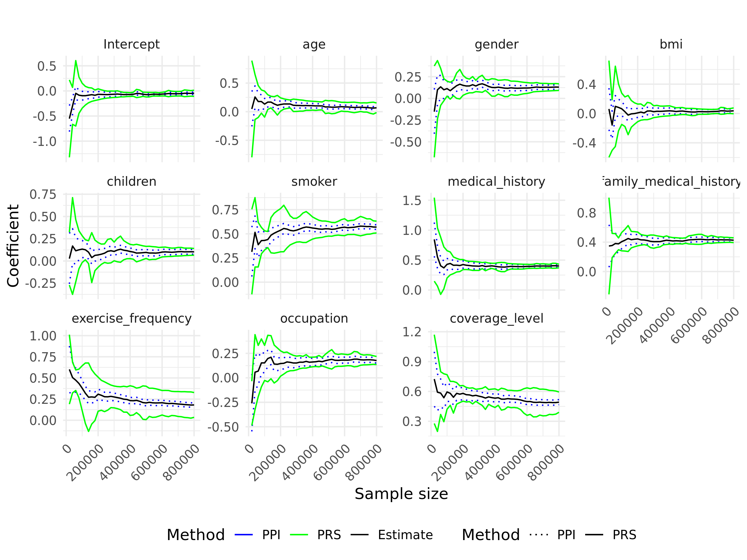
The results demonstrate that as the sample size increases, all regression coefficients for predicting health insurance premiums converge to positive values, indicating their significant contributions to premium determination. A positive coefficient implies that higher values of a predictor correspond to higher premiums. For instance, males are charged higher premiums than females, smokers incur substantially higher costs due to increased health risks, and individuals with serious medical conditions or a family history of such conditions (e.g., diabetes, heart disease) face elevated premiums. Likewise, a higher BMI and selecting more comprehensive insurance plans also lead to higher charges, reflecting the associated health risks or benefits. While the coefficients for age and exercise frequency are positive, their magnitudes are relatively small, suggesting a limited linear effect on premium pricing. Its influence may be non-linear and not fully captured by a simple linear term. Overall, the analysis highlights that risk-related factors such as smoking, BMI, and medical history, are the primary drivers of health insurance premiums, while demographic and lifestyle factors exert a lesser influence.
We apply the LDP-SGD estimator to perform linear regression for predicting insurance charges. The mean squared error (MSE) on the test set is 0.0722. For comparison, we also fit an offline ordinary least squares (OLS) estimator without privacy guarantees using the same training data, which achieves an MSE of 0.0607. Table 3 summarizes the comparison between the LDP-SGD and offline OLS estimators in terms of coefficient estimates. The results show that LDP-SGD estimators closely align with OLS estimates, indicating that the proposed algorithm effectively protects privacy while preserving utility and explanatory power.
| Setting | age | gender | bmi | children | smoker |
|---|---|---|---|---|---|
| OLS | 0.0627 | 0.1131 | 0.1044 | 0.0774 | 0.5659 |
| LDP-SGD | 0.0679 | 0.1298 | 0.0664 | 0.0828 | 0.5483 |
| Setting | medical | family medical | exercise | occupation | coverage level |
| OLS | 0.4052 | 0.4051 | 0.1389 | 0.1516 | 0.4625 |
| LDP-SGD | 0.4009 | 0.4264 | 0.1409 | 0.1767 | 0.4634 |
7 Discussion
This paper investigates online private estimation and inference for optimization-based problems with streaming data under local differential privacy constraints. To eliminate the dependence on trusted data collectors, we propose an LDP-SGD algorithm that processes data in a single pass, making it well-suited for streaming applications and minimizing storage costs. Additionally, we introduce and discuss three asymptotically valid online private inference methods—private plug-in, private batch-means, and random scaling—for constructing private confidence intervals. We establish the consistency and asymptotic normality of the proposed estimators, providing a theoretical foundation for our online private inference approach.
Several directions for future research are worth exploring. First, while this work focuses on low-dimensional settings, extending the methodology to high-dimensional penalized estimators using noisy proximal methods would be valuable. Second, our models are based on parametric assumptions; adapting these to non-parametric models by developing a noisy functional SGD algorithm remains interesting. Finally, this work assumes strong convexity and smoothness of the objective loss function. However, extending the proposed framework to encompass general nonsmooth convex functions, such as ReLU and quantile losses, which are piecewise linear and lack strong convexity, call for future research.
References
- Abadir and Paruolo (1997) Abadir, K. M. and P. Paruolo (1997). Two mixed normal densities from cointegration analysis. Econometrica: Journal of the Econometric Society, 671–680.
- Alabi and Vadhan (2023) Alabi, D. G. and S. P. Vadhan (2023). Differentially private hypothesis testing for linear regression. Journal of Machine Learning Research 24(361), 1–50.
- Avella-Medina (2021) Avella-Medina, M. (2021). Privacy-preserving parametric inference: a case for robust statistics. Journal of the American Statistical Association 116(534), 969–983.
- Avella-Medina et al. (2023) Avella-Medina, M., C. Bradshaw, and P.-L. Loh (2023). Differentially private inference via noisy optimization. The Annals of Statistics 51(5), 2067–2092.
- Barrientos et al. (2019) Barrientos, A. F., J. P. Reiter, A. Machanavajjhala, and Y. Chen (2019). Differentially private significance tests for regression coefficients. Journal of Computational and Graphical Statistics 28(2), 440–453.
- Berrett and Yu (2021) Berrett, T. and Y. Yu (2021). Locally private online change point detection. Advances in Neural Information Processing Systems 34, 3425–3437.
- Chadha et al. (2021) Chadha, K., J. Duchi, and R. Kuditipudi (2021). Private confidence sets. In NeurIPS 2021 Workshop Privacy in Machine Learning.
- Chen et al. (2024) Chen, X., Z. Lai, H. Li, and Y. Zhang (2024). Online statistical inference for stochastic optimization via kiefer-wolfowitz methods. Journal of the American Statistical Association, 1–24.
- Chen et al. (2020) Chen, X., J. D. Lee, X. T. Tong, and Y. Zhang (2020). Statistical inference for model parameters in stochastic gradient descent. The Annals of Statistics 48(1), 251–273.
- Dankar and El Emam (2013) Dankar, F. K. and K. El Emam (2013). Practicing differential privacy in health care: A review. Trans. Data Priv. 6(1), 35–67.
- Davidow et al. (2023) Davidow, D. M., Y. Manevich, and E. Toch (2023). Privacy-preserving transactions with verifiable local differential privacy. In 5th Conference on Advances in Financial Technologies.
- Ding et al. (2017) Ding, B., J. Kulkarni, and S. Yekhanin (2017). Collecting telemetry data privately. Advances in Neural Information Processing Systems 30.
- Dong et al. (2022) Dong, J., A. Roth, and W. J. Su (2022). Gaussian differential privacy. Journal of the Royal Statistical Society Series B: Statistical Methodology 84(1), 3–37.
- Duchi et al. (2018) Duchi, J. C., M. I. Jordan, and M. J. Wainwright (2018). Minimax optimal procedures for locally private estimation. Journal of the American Statistical Association 113(521), 182–201.
- Dwork et al. (2006) Dwork, C., F. McSherry, K. Nissim, and A. Smith (2006). Calibrating noise to sensitivity in private data analysis. In Theory of Cryptography: Third Theory of Cryptography Conference, TCC 2006, New York, NY, USA, March 4-7, 2006. Proceedings 3, pp. 265–284. Springer.
- Erlingsson et al. (2014) Erlingsson, Ú., V. Pihur, and A. Korolova (2014). Rappor: Randomized aggregatable privacy-preserving ordinal response. In Proceedings of the 2014 ACM SIGSAC conference on computer and communications security, pp. 1054–1067.
- Fainmesser et al. (2023) Fainmesser, I. P., A. Galeotti, and R. Momot (2023). Digital privacy. Management Science 69(6), 3157–3173.
- Hu et al. (2022) Hu, M., R. Momot, and J. Wang (2022). Privacy management in service systems. Manufacturing & Service Operations Management 24(5), 2761–2779.
- Karwa and Slavković (2016) Karwa, V. and A. Slavković (2016). Inference using noisy degrees: Differentially private -model and synthetic graphs. The Annals of Statistics 44(1), 87–112.
- Karwa and Vadhan (2018) Karwa, V. and S. Vadhan (2018). Finite sample differentially private confidence intervals. In 9th Innovations in Theoretical Computer Science Conferenc 94.
- Lee et al. (2022) Lee, S., Y. Liao, M. H. Seo, and Y. Shin (2022). Fast and robust online inference with stochastic gradient descent via random scaling. In Proceedings of the AAAI Conference on Artificial Intelligence, Volume 36, pp. 7381–7389.
- Li et al. (2024) Li, M., Y. Tian, Y. Feng, and Y. Yu (2024). Federated transfer learning with differential privacy. arXiv preprint arXiv:2403.11343.
- Li et al. (2022) Li, X., J. Liang, X. Chang, and Z. Zhang (2022). Statistical estimation and online inference via local sgd. In Conference on Learning Theory, pp. 1613–1661. PMLR.
- Lin and Xi (2011) Lin, N. and R. Xi (2011). Aggregated estimating equation estimation. Statistics and its Interface 4(1), 73–83.
- Liu et al. (2023) Liu, Y., Q. Hu, L. Ding, and L. Kong (2023). Online local differential private quantile inference via self-normalization. In International Conference on Machine Learning, pp. 21698–21714. PMLR.
- Luo and Song (2020) Luo, L. and P. X.-K. Song (2020). Renewable estimation and incremental inference in generalized linear models with streaming data sets. Journal of the Royal Statistical Society Series B: Statistical Methodology 82(1), 69–97.
- Man et al. (2024) Man, R., K. M. Tan, Z. Wang, and W.-X. Zhou (2024). Retire: Robust expectile regression in high dimensions. Journal of Econometrics 239(2), 105459.
- Maniar et al. (2021) Maniar, T., A. Akkinepally, and A. Sharma (2021). Differential privacy for credit risk model. arXiv preprint arXiv:2106.15343.
- Polyak and Juditsky (1992) Polyak, B. T. and A. B. Juditsky (1992). Acceleration of stochastic approximation by averaging. SIAM journal on control and optimization 30(4), 838–855.
- Ponomareva et al. (2023) Ponomareva, N., H. Hazimeh, A. Kurakin, Z. Xu, C. Denison, H. B. McMahan, S. Vassilvitskii, S. Chien, and A. G. Thakurta (2023). How to dp-fy ml: A practical guide to machine learning with differential privacy. Journal of Artificial Intelligence Research 77, 1113–1201.
- Robbins and Monro (1951) Robbins, H. and S. Monro (1951). A stochastic approximation method. The Annals of Mathematical Statistics, 400–407.
- Rohde and Steinberger (2020) Rohde, A. and L. Steinberger (2020). Geometrizing rates of convergence under local differential privacy constraints. The Annals of Statistics 48(5), 2646–2670.
- Ruppert (1988) Ruppert, D. (1988). Efficient estimations from a slowly convergent robbins-monro process. Technical report, Cornell University Operations Research and Industrial Engineering.
- Sart (2023) Sart, M. (2023). Density estimation under local differential privacy and hellinger loss. Bernoulli 29(3), 2318–2341.
- Schifano et al. (2016) Schifano, E. D., J. Wu, C. Wang, J. Yan, and M.-H. Chen (2016). Online updating of statistical inference in the big data setting. Technometrics 58(3), 393–403.
- Sheffet (2017) Sheffet, O. (2017). Differentially private ordinary least squares. In International Conference on Machine Learning, pp. 3105–3114. PMLR.
- Smith et al. (2022) Smith, J., H. J. Asghar, G. Gioiosa, S. Mrabet, S. Gaspers, and P. Tyler (2022). Making the most of parallel composition in differential privacy. Proceedings on Privacy Enhancing Technologies, 253–273.
- Song et al. (2021) Song, S., T. Steinke, O. Thakkar, and A. Thakurta (2021). Evading the curse of dimensionality in unconstrained private glms. In International Conference on Artificial Intelligence and Statistics, pp. 2638–2646. PMLR.
- Tang et al. (2017) Tang, J., A. Korolova, X. Bai, X. Wang, and X. Wang (2017). Privacy loss in apple’s implementation of differential privacy on macos 10.12. arXiv preprint arXiv:1709.02753.
- Vaswani et al. (2022) Vaswani, S., B. Dubois-Taine, and R. Babanezhad (2022). Towards noise-adaptive, problem-adaptive (accelerated) stochastic gradient descent. In International conference on machine learning, pp. 22015–22059. PMLR.
- Wang et al. (2019) Wang, Y., D. Kifer, and J. Lee (2019). Differentially private confidence intervals for empirical risk minimization. Journal of Privacy and Confidentiality 9.
- Wang and Tsai (2022) Wang, Y.-R. and Y.-C. Tsai (2022). The protection of data sharing for privacy in financial vision. Applied Sciences 12(15), 7408.
- Zhang et al. (2024) Zhang, Z., R. Nakada, and L. Zhang (2024). Differentially private federated learning: Servers trustworthiness, estimation, and statistical inference. arXiv preprint arXiv:2404.16287.
- Zhao et al. (2024) Zhao, T., W. Zhou, and L. Wang (2024). Private optimal inventory policy learning for feature-based newsvendor with unknown demand. Management Science, in press.
- Zhong (2019) Zhong, G. (2019). E-commerce consumer privacy protection based on differential privacy. In Journal of Physics: Conference Series, Volume 1168, pp. 032084. IOP Publishing.
- Zhu et al. (2023) Zhu, W., X. Chen, and W. B. Wu (2023). Online covariance matrix estimation in stochastic gradient descent. Journal of the American Statistical Association 118(541), 393–404.