Online Guaranteed Reachable Set Approximation for Systems with Changed Dynamics and Control Authority

Hamza El-Kebir \IEEEmembershipStudent Member, IEEE Ani Pirosmanishvili Melkior Ornik \IEEEmembershipMember, IEEE Manuscript received September 25, 2021. H. El-Kebir is with the Dept. of Aerospace Engineering at the University of Illinois Urbana-Champaign, Urbana, IL 61801 USA (e-mail: elkebir2@illinois.edu). A. Pirosmanishvili is with the Dept. of Aerospace Engineering at the University of Illinois Urbana-Champaign, Urbana, IL 61801 USA (e-mail: anip2@illinois.edu). M. Ornik is with the Dept. of Aerospace Engineering and the Coordinated Science Laboratory at the University of Illinois Urbana-Champaign, Urbana, IL 61801 USA (e-mail: mornik@illinois.edu).

Abstract

This work presents a method of efficiently computing inner and outer approximations of forward reachable sets for nonlinear control systems with changed dynamics and diminished control authority, given an a priori computed reachable set for the nominal system. The method functions by shrinking or inflating a precomputed reachable set based on prior knowledge of the system’s trajectory deviation growth dynamics, depending on whether an inner approximation or outer approximation is desired. These dynamics determine an upper bound on the minimal deviation between two trajectories emanating from the same point that are generated on the nominal system using nominal control inputs, and by the impaired system based on the diminished set of control inputs, respectively. The dynamics depend on the given Hausdorff distance bound between the nominal set of admissible controls and the possibly unknown impaired space of admissible controls, as well as a bound on the rate change between the nominal and off-nominal dynamics. Because of its computational efficiency compared to direct computation of the off-nominal reachable set, this procedure can be applied to on-board fault-tolerant path planning and failure recovery. In addition, the proposed algorithm does not require convexity of the reachable sets unlike our previous work, thereby making it suitable for general use. We raise a number of implementational considerations for our algorithm, and we present three illustrative examples, namely an application to the heading dynamics of a ship, a lower triangular dynamical system, and a system of coupled linear subsystems.

{IEEEkeywords}

Reachability analysis, guaranteed reachability, safety-critical control, computation and control.

1 Introduction

\IEEEPARstart

Reachability analysis forms a fundamental part of dynamical system analysis and control theory, providing a means to assess the set of states that a system can reach under admissible control inputs at a certain point in time from a given set of initial states. Inner approximations of reachable sets are often used to attain a guaranteed estimate of the system’s capabilities, while outer approximations can be used to verify that the system will not reach an unsafe state.

Outer approximations find widespread applications in fault-tolerance analysis and formal verification [1], safe trajectory planning [2], and constrained feedback controller synthesis [3]. Methods for computing outer approximations of the reachable set include polynomial overapproximation [4], direct set propagation [5], and viscosity solutions to Hamilton–Jacobi–Bellman (HJB) equations [6].

Inner approximations of reachable sets have received comparatively less attention than outer approximations [7], but have recently seen use in path-planning problems with collision avoidance [8], as well as viability kernel computation [9], which can in turn be used for guaranteed trajectory planning [10]. Another application lies in safe set determination, in which one aims to obtain an inner approximation of the maximal robust control invariant set [11]. Methods for determining inner approximations of reachable sets have been based on various principles, including relying on polynomial inner approximation of the nonlinear system dynamics using interval calculus [12], ellipsoid calculus [13], and viscosity solutions to HJB equations [14]. One major drawback of these methods is that they are computationally intensive and are often only suitable for systems of low dimension, making them ill-suited for online use.

In this work, we consider the problem of obtaining meaningful approximations of the reachable set of an off-nominal system by leveraging available a priori information on the nominal system dynamics. Here, we consider the reachable set of the nominal system, or an inner/outer approximation thereof, to be known prior to the system’s operation. While obtaining reachable sets is often a computationally intensive task, it is often done during the design phase of a system, where computation times are less of a concern [15]. We then consider a change in dynamics of the system, for example due to partial system failure, which turns the nominal system into the off-nominal system. Our goals is to obtain inner and outer approximations of the off-nominal reachable sets based on the nominal reachable set, in a way that can be applied in real-time.

In [16], the case in which the system experiences diminished control authority was considered, i.e., its set of admissible control inputs has shrunk with respect to that of the nominal system. In addition, stringent restrictions on the family of system that could be considered were made in [16], in particular due to the requirement that the reachable set for the nominal and off-nominal set be convex. This ultimately limits the applicability of the theory presented there to a limited set of problems.

Here, we do not impose any demands on the convexity of the reachable set, while still presenting an algorithm that can be run in real-time. This latter generalization to nonconvex sets requires a significant shift in the way we reason about the minimum deviation between trajectories of the nominal and off-nominal system. In this work, we also consider a change in the system dynamics, and provide methods for obtaining tighter inner and outer approximations for the off-nominal reachable set with respect to what the theory of [16] provides. This latter improvement follows from the fact that the theory in [16] considers the trajectory deviation as expressed by the norm of the states, whereas here we separately consider the deviation in single dimensions of the state.

To obtain inner and outer approximations of the off-nominal reachable set, we consider that an upper bound on the minimal rate of change of the trajectory deviation between the off-nominal system’s trajectories with respect to those of the nominal system’s is known, with both trajectories emanating from the same point. These growth dynamics provide an upper bound on the minimal rate of change between two trajectories emanating from the same point, with one trajectory being generated by the nominal set of control inputs, and the other by the off-nominal set of control inputs and the off-nominal dynamics. An upper bound on these growth dynamics can be obtained analytically during the design phase, and allows us to obtain an inner approximation to the off-nominal system’s reachable set at low computational cost, in an online manner.

While other methods have been proposed to compute reachable sets under system impairment, due to their computational complexity, these have either used reduced order models, or have been limited to offline applications [17]. In more extreme cases of system impairments, such as those were very little is known about the system’s present capabilities, more conservative methods for computing reachable sets exist [18]. Here, we present a general algorithm that yields guaranteed inner and outer approximations, given limited knowledge of the failure modes as expressed by a bound on the trajectory deviation growth dynamics. We leverage the fact that the off-nominal system dynamics are related to the nominal system’s dynamics, allowing us to leverage reachable sets computed for the nominal system, unlike in [18]. Given a sufficiently tight deviation growth bound, our approach can be applied online to high dimensional systems with no additional computational cost for the growth in system dimension.

The paper is organized as follows. First, we present preliminary theory in Section 2. Then, we present our main results Section 3, followed by a simulation example involving the heading dynamics of ship, as well as two general scalable system examples, in Section 4. Finally, we draw conclusions in Section 5. In Appendix 6, we present a slightly more relaxed set of assumptions under which the theory presented continues to hold.

2 Preliminaries

In the following, we denote by $\|\cdot\|$ the Euclidean norm. Given two sets $A,B\subseteq\mathbb{R}^{n}$ , we denote by $A\oplus B$ Minkowski sum $\{a+b:a\in A,b\in B\}$ . We denote a ball centered around the origin with radius $r>0$ as $\mathcal{B}_{r}$ . By $\mathcal{B}(x,r)$ we denote $\{x\}\oplus\mathcal{B}_{r}$ . We denote by ‘ $\operatorname*{\scalerel*{\times}{\sum}}$ ’ the Cartesian product. We define $\mathbb{R}_{+}:=[0,\infty)$ . We define the distance between two sets $A,B\subseteq\mathbb{R}^{n}$ to be

d(A,B):=\sup_{a\in A}\inf_{b\in B}d(a,b),

(1)

where $d$ is the Euclidean metric. We denote the Hausdorff distance as

d_{\mathrm{H}}(A,B):=\max\{d(A,B),d(B,A)\},

(2)

where $d$ is the Euclidean metric. An alternative characterization of the Hausdorff distance reads [19, pp. 280–281]:

d_{\mathrm{H}}(A,B)=\inf\{\rho\geq 0:A\subseteq B_{+\rho},B\subseteq A_{+\rho}\},

(3)

where $X_{+\rho}$ denotes the $\rho$ -fattening of $X$ , i.e., $X_{+\rho}:=\bigcup_{x\in X}\{y\in\mathbb{R}^{n}:\|x-y\|\leq\rho\}$ .

Given a point $x\in S$ and a set $A\subseteq S$ , we denote $d(x,A):=\inf_{y\in A}d(x,y)$ . We denote by $\partial A$ the boundary of $A$ in the topology induced by the Euclidean norm. For a function $g:A\to B$ , we denote by $g^{-1}$ the inverse of this function if an inverse exists, and by $\mathrm{dom}(g)$ the domain of the function (in this case $A$ ). We denote a multifunction by $G:A\rightrightarrows B$ , where $G$ maps elements of $A$ to subsets of $B$ . Given a multifunction $G$ , we define a differential inclusion as being the set of ordinary differential equations $\dot{x}\in G(x)$ that have velocities in $G(x)$ .

Given two vectors $u,v\in\mathbb{R}^{n}$ , we denote by $u\preceq v$ a component-wise nonstrict inequality, i.e., $u_{i}\leq v_{i}$ for $i=1,\ldots,n$ . By $|u|$ , we denote a component-wise absolute value, such that $|u|_{i}=|u_{i}|$ . Given a set $Y$ , we denote its cardinality by $\#Y$ . We use the abbreviation ‘a.e.’ (almost every) to refer to statements that are true everywhere except potentially on some zero-measure sets. Given a real value $a\in\mathbb{R}$ we denotes its ceiling by $\lceil a\rceil=\min([a,\infty)\cap\mathbb{N})$ . For a closed interval $[a,b]\subseteq\mathbb{R}$ , we denote its length by $\mathrm{length}([a,b]):=b-a$ . Given $N$ matrices $A^{(1)},\ldots,A^{(N)}$ , with $A^{(i)}\in\mathbb{R}^{n_{i}\times m_{i}}$ for each $i=1,\ldots,n$ , we define $\mathrm{diag}(\{A^{(1)},\ldots,A^{(N)}\})$ to be the block diagonal matrix formed by these matrices.

2.1 Problem Statement

Consider a dynamical system of the form

\begin{split}\dot{x}(t)&=f(x(t),u(t)),\\ x(0)&=x_{0},\end{split}

(4)

where $t\geq 0$ , $x\in\mathbb{R}^{n}$ is the state, and $u\in\mathscr{U}\subseteq\mathbb{R}^{m}$ is the control input, where $\mathscr{U}$ is some admissible set of control inputs. The dynamics have the form $f:\mathbb{R}^{n}\times\mathscr{U}\to\mathbb{R}^{n}$ . We refer to these dynamics as the ‘nominal’ dynamics.

We consider an impairment in the system dynamics, as well as the system’s control authority, such that $\bar{u}(t)\in\bar{\mathscr{U}}\subseteq\mathscr{U}\subseteq\mathbb{R}^{m}$ . The modified dynamics then read:

\begin{split}\dot{\bar{x}}(t)&=g(\bar{x}(t),\bar{u}(t)),\\ \bar{x}(0)&=x_{0}.\end{split}

(5)

We refer to these modified dynamics as the ‘off-nominal’ dynamics.

Definition 1 (Forward reachable set).

We define a function $\phi:\mathbb{R}_{+}\to\mathscr{U}$ as an admissible input signal, if a unique solution to (4) exists given that input signal. The set of admissible control signals is defined as all possible admissible input signals $\mathbb{U}:=\{\phi:\mathbb{R}_{+}\to\mathscr{U}\}$ .

We define a trajectory $\varphi:\mathbb{R}_{+}\times\mathbb{R}^{n}\times\mathbb{U}\to\mathbb{R}^{n}$ to be such that $x(t)=\varphi(t|x_{0},\phi)$ satisfies (4) given initial state $x(0)=x_{0}\in\mathbb{R}^{n}$ and input signal $u(t)=\phi(t)\in\mathbb{U}$ , i.e.,

\varphi(t|x_{0},\phi):=x_{0}+\int_{0}^{t}f(x(\tau),\phi(\tau))\ \mathrm{d}\tau.

From the dynamics of (4), we define a multifunction $F(t,x):=f(t,x,\mathscr{U}):\mathbb{R}_{+}\times\mathbb{R}^{n}\rightrightarrows\mathbb{R}^{n}$ . This multifunction defines an ordinary differential inclusion $\dot{x}(t)\in F(t,x(t))$ , of which any instance of (4) is a part. We define the solution set of this ordinary differential inclusion as follows:

S_{F}(x_{0}):=\{\varphi(\cdot|x_{0},\phi):x_{0}\in\mathscr{X}_{0},\phi\in\mathbb{U}\}.

Given a set of initial states $\mathscr{X}_{0}\subseteq\mathbb{R}^{n}$ , we define the forward reachable set (FRS) at time $\tau\in\mathbb{R}_{+}$ as

\begin{split}\mathbb{X}_{\tau}^{\rightarrow}(F,\mathscr{X}_{0})&:=\bigcup_{x\in\mathscr{X}_{0}}\{x(\tau):x\in S_{F}(x_{0})\}\\ &=\{\varphi(\tau|x_{0},\phi):x_{0}\in\mathscr{X}_{0},\phi\in\mathbb{U}\}.\end{split}

We consider the following main problem, comprised of two parts: one relating to obtaining inner approximations of reachable sets, and the other concerned with obtaining outer approximations of reachable sets. In this work, we treat both the case of impaired control authority, as well as changed dynamics, simultaneously.

Problem 1 (Off-nominal FRS approximation).

Given the nominal dynamics $\dot{x}(t)=f(x(t),u(t)),$ the off-nominal dynamics $\dot{\bar{x}}(t)=g(\bar{x}(t),\bar{u}(t)),$ a set of admissible control inputs $\mathscr{U}$ , (an inner (outer) approximation of the) forward reachable set $\mathbb{X}_{\tau}^{\rightarrow}$ at time $\tau$ , and the corresponding initial set of states $\mathscr{X}_{f}$ , find an inner (outer) approximation of the reachable set at time $\tau$ , $\bar{\mathbb{X}}_{\tau}^{\rightarrow}$ , for the dynamics $\dot{\bar{x}}(t)=g(\bar{x}(t),\bar{u}(t))$ and the admissible control inputs $\bar{\mathscr{U}}=h(\mathscr{U})$ , for some control mapping $h:\mathscr{U}\to\bar{\mathscr{U}}$ .

As mentioned in the introduction, inner approximations of the off-nominal reachable set are useful for safety critical control, when guaranteed reachability is demanded. However, when dealing with collision avoidance, outer approximations of the off-nominal reachable set of a moving target are needed. This justifies the need for two separate approximation objectives.

2.2 Generalized Nonlinear Trajectory Deviation Growth Bound

As mentioned in the introduction, we wish to find an upper bound on the minimum normed distance between two trajectories emanating from the same, once governed by (4), and the other by (8). We call this upper bound the trajectory deviation growth bound. To this end, we first consider a means of obtaining and upper bound to the norm of the solution of a given ordinary differential equation (ODE). This particular ODE will be described by the rate of change of the deviation between two trajectories, which we refer to as the trajectory deviation growth dynamics, as will be described shortly.

We consider the following general nonlinear time-varying dynamics

\dot{x}(t)=h(t,x(t),u(t)),\quad x(0)=x_{0}\in\mathbb{R}^{n},

(6)

Our goal is to find an upper bound for the magnitude of $x(t)$ , given particular assumptions on the form of control input $u$ and the function $h$ , over a finite period of time. We make the following assumption on the growth rate of $x$ :

Assumption 1.

For all $x\in\mathbb{R}^{n}$ , $u\in\mathscr{U}$ , $t_{0}\leq t<\infty$

\|h(t,x,u)\|\leq a(t)w(\|x\|,\|u\|)+b(t),

where $a,b$ are continuous and positive and $w$ is continuous, monotonic, nondecreasing and positive. In addition, $w$ is uniformly monotonically nondecreasing in $\|u\|$ .

Theorem 1 (Extended Bihari inequality [16, Theorem 3.1]).

Let $x(t)$ be a solution to the equation

\dot{x}=h(t,x,u),\quad 0\leq t_{0}\leq t<\infty,

where $h(t,x,u):[t_{0},\infty)\times\mathbb{R}^{n}\times\mathscr{U}\to\mathbb{R}^{n}$ is continuous for $t_{0}\leq t<\infty$ , and $\mathscr{U}\subseteq\mathbb{R}^{m}$ is compact and satisfies $\max_{u\in\mathscr{U}}\|u\|=\delta$ . Let Assumption 1 hold. Then,

\|x(t)\|\leq G^{-1}\left[G\left(\|x(t_{0})\|+\int_{t_{0}}^{t}b(\tau)\mathrm{d}\tau\right)+\int_{t_{0}}^{t}a(\tau)\mathrm{d}\tau\right],

(7)

where the expression on the right-hand side is strictly increasing in $t$ . In (7), we define

G(r):=\int_{r_{0}}^{r}\frac{\mathrm{d}s}{w(s,\delta)},\quad r>0,r_{0}>0,

for arbitrary $r_{0}>0$ and for all $t\geq t_{0}$ for which it holds that

G\left(\|x(t_{0})\|+\int_{t_{0}}^{t}b(\tau)\mathrm{d}\tau\right)+\int_{t_{0}}^{t}a(\tau)\mathrm{d}\tau\in\mathrm{dom}(G^{-1}).

Remark 1.

Theorem 1 is a generalization of the Gronwall–Bellman inequality. It can be reduced to the Gronwall-Bellman inequality by taking $w(u)=u$ and $G(u)=\log u$ (see [20, Remark 2.3.2, p. 109] for a more in-depth discussion).

Corollary 1.

For any $x_{0}\in\mathscr{X}_{0}\subseteq\mathbb{R}^{n}$ , where $\mathscr{X}_{0}$ is compact, and any initial time $t_{\mathrm{init}}\in[t_{0},\infty)$ and final time $t_{f}\in[t_{\mathrm{init}},\infty)$ , consider a trajectory $x(t)$ satisfying $x(t_{\mathrm{init}})=x_{0}$ and $\dot{x}(t)=f(t,x(t),u(t))$ , with $u(t)\in\mathbb{U}$ . Consider a trajectory $\bar{x}(t)$ with $\bar{x}(t_{\mathrm{init}})=x_{0}$ and $\dot{\bar{x}}(t)=f(t,\bar{x}(t),\bar{u}(t))$ , such that $\bar{u}(t)\in\bar{\mathbb{U}}$ satisfies $\sup_{t\in[t_{\mathrm{init}},t_{f}]}\|u(t)-\bar{u}(t)\|\leq\epsilon$ . Let $\tilde{f}(t):=f(t,x(t),u(t))-f(t,\bar{x}(t),\bar{u}(t))$ , $\tilde{x}(t):=x(t)-\bar{x}(t)$ , and $\tilde{u}(t):=u(t)-\bar{u}(t)$ . Let the following bound hold for $t\in[t_{\mathrm{init}},t_{f}]$ , and for any $x(t)$ and $\bar{x}(t)$ satisfying the previous hypotheses: $\|\tilde{f}(t)\|\leq\tilde{a}(t)\tilde{w}(\|\tilde{x}(t)\|,\|\tilde{u}(t)\|)+\tilde{b}(t)$ with $\tilde{a},\tilde{b},\tilde{w}$ satisfying the assumptions given in Assumption 1. Then, $\tilde{x}(t)$ satisfies

\|\tilde{x}(t)\|\leq G^{-1}\left[G\left(\int_{t_{0}}^{t}\tilde{b}(\tau)\mathrm{d}\tau\right)+\int_{t_{0}}^{t}\tilde{a}(\tau)\mathrm{d}\tau\right]=:\eta(t,\epsilon)

for all $t\in[t_{\mathrm{init}},t_{f}]$ .

Proof.

Given the premise, this claim follows directly from Theorem 1. $\square$ ∎

Corollary 2.

For any $x_{0}\in\mathscr{X}_{0}\subseteq\mathbb{R}^{n}$ , where $\mathscr{X}_{0}$ is compact, and any initial time $t_{\mathrm{init}}\in[t_{0},\infty)$ and final time $t_{f}\in[t_{\mathrm{init}},\infty)$ , consider a trajectory $x(t)$ satisfying $x(t_{\mathrm{init}})=x_{0}$ and $\dot{x}(t)=f(t,x(t),u(t))$ , with $u(t)\in\mathbb{U}$ . Consider a trajectory $\bar{x}(t)$ with $\bar{x}(t_{\mathrm{init}})=\bar{x}_{0}$ , where $\bar{x}_{0}\in\bar{\mathscr{X}}_{0}\subseteq\mathbb{R}^{n}$ , and $\dot{\bar{x}}(t)=f(t,\bar{x}(t),\bar{u}(t))$ , such that $\bar{u}(t)\in\bar{\mathbb{U}}$ satisfies $\sup_{t\in[t_{\mathrm{init}},t_{f}]}\|u(t)-\bar{u}(t)\|\leq\epsilon$ . Let $\tilde{f}(t):=f(t,x(t),u(t))-f(t,\bar{x}(t),\bar{u}(t))$ , $\tilde{x}(t):=x(t)-\bar{x}(t)$ , and $\tilde{u}(t):=u(t)-\bar{u}(t)$ . Let $d_{\text{H}}(\mathscr{X}_{0},\bar{\mathscr{X}}_{0})\leq\kappa$ . Let the following bound hold for $t\in[t_{\mathrm{init}},t_{f}]$ , and for any $x(t)$ and $\bar{x}(t)$ satisfying the previous hypotheses: $\|\tilde{f}(t)\|\leq\tilde{a}(t)\tilde{w}(\|\tilde{x}(t)\|,\|\tilde{u}(t)\|)+\tilde{b}(t)$ with $\tilde{a},\tilde{b},\tilde{w}$ satisfying the assumptions given in Assumption 1. Then, $\tilde{x}(t)$ satisfies

\begin{split}\|\tilde{x}(t)\|&\leq G^{-1}\left[G\left(\kappa+\int_{t_{0}}^{t}\tilde{b}(\tau)\mathrm{d}\tau\right)+\int_{t_{0}}^{t}\tilde{a}(\tau)\mathrm{d}\tau\right]\\ &=:\eta(t,\epsilon,\kappa)\end{split}

for all $t\in[t_{\mathrm{init}},t_{f}]$ .

Proof.

Similarly to Corollary 1, given the premise, this claim follows directly from Theorem 1. $\square$ ∎

2.2.1 Generalization to off-nominal dynamics

We now consider the following nonlinear time-varying off-nominal dynamics:

\dot{x}(t)=g(t,x(t),u(t)),\quad x(0)=x_{0}\in\mathbb{R}^{n},

(8)

which gives rise to the following assumption that relates these unknown dynamics to the known nominal system dynamics:

Assumption 2.

For all $x\in\mathbb{R}^{n}$ , $u\in\mathscr{U}$ , $t_{0}\leq t<\infty$ , we have

\|g(t,x,u)-f(t,x,u)\|\leq\gamma(t),

where $\gamma$ is a positive, continuous function on $[t_{0},\infty)$ .

This assumption gives rise to the following lemma

Lemma 1.

Let Assumption 2 hold true. Consider functions $\bar{a},\bar{b},\bar{w}$ , in the sense of Assumption 1, which apply to the following dynamics

\dot{\tilde{x}}(t)=f(t,x(t)+\tilde{x}(t),u(t)+\tilde{u}(t))-f(t,x(t),u(t)),\quad\tilde{x}(t_{0})=0.

We consider nominal control signal $u\in\mathbb{U}_{\epsilon}$ , and an off-nominal control signal of the form $(u+\bar{u})\in\mathbb{U}$ are such that $\sup_{\bar{u}(t),t\in[t_{0},\infty)}\|\bar{u}(t)\|\leq\epsilon$ .

In addition, consider the following off-nominal trajectory deviation dynamics:

\dot{\hat{x}}(t)=g(t,x(t)+\hat{x}(t),u(t)+\hat{u}(t))-f(t,x(t),u(t)),\quad\hat{x}(t_{0})=0.

Control signals $u$ and $\hat{u}$ are defined similarly to those of the nominal dynamics. We have a nominal control signal $u\in\mathbb{U}_{\epsilon}$ , and an off-nominal control signal of the form $(u+\hat{u})\in\mathbb{U}$ such that $\sup_{\hat{u}(t),t\in[t_{0},\infty)}\|\hat{u}(t)\|\leq\epsilon$ .

We define $\hat{b}(t):=\tilde{b}(t)+\gamma(t)$ . We have that $\|\tilde{x}(t)\|\leq\eta(t,\epsilon)$ , where $\eta(t,\epsilon)$ is obtained as in Corollary 1 with $\tilde{a}=\bar{a}$ , $\tilde{b}=\hat{b}$ , $\tilde{w}=\bar{w}$ .

Proof.

This result follows straightforwardly by application of the the triangle inequality on the trajectory deviation growth dynamics and Corollary 1. $\square$ ∎

3 Main results

We now present the main results of this paper. We give a method for inner and outer approximation of the forward reachable sets for off-nominal systems that are subject to both diminishment of control authority and changed dynamics.

Unlike in [16], a new hyperrectangular version of the Bihari inequality is required to obtain inner and outer approximations to more generalized reachable sets. As will be specified later, the only requirements imposed on these reachable sets will be that they are nonempty, compact, and connected. To construct a hyperrectangular Bihari inequality, we present a modified nonlinear bound on the deviation dynamics:

Definition 2 ( $(a_{i},b_{i},w_{i})$ -bounded growth).

We say that a function $h:[t_{0},\infty)\times\mathbb{R}^{n}\times\mathscr{U}\to\mathbb{R}^{n}$ has $(a_{i},b_{i},w_{i})$ -bounded growth if for all $x\in\mathbb{R}^{n}$ , $u\in\mathscr{U}$ , $t_{0}\leq t<\infty$ , the following inequality holds:

|h_{i}(t,x,u)|\leq a_{i}(t)w_{i}(|x_{i}|,\|u\|)+b_{i}(t),

for each $i\in\{1,\ldots,n\}$ , where $a_{i},b_{i}$ are continuous and positive and $w_{i}$ is continuous, monotonic, nondecreasing and positive in both of its arguments.

Given this definition, we can now formulate a generalization to Corollary 1:

Lemma 2.

For any $x_{0}\in\mathscr{X}_{0}\subseteq\mathbb{R}^{n}$ , where $\mathscr{X}_{0}$ is compact, and any initial time $t_{\mathrm{init}}\in[t_{0},\infty)$ and final time $t_{f}\in[t_{\mathrm{init}},\infty)$ , consider a trajectory $x(t)$ satisfying $x(t_{\mathrm{init}})=x_{0}$ and $\dot{x}(t)=f(t,x(t),u(t))$ , with $u(t)\in\mathbb{U}$ . Consider a trajectory $\bar{x}(t)$ with $\bar{x}(t_{\mathrm{init}})=x_{0}$ and $\dot{\bar{x}}(t)=f(t,\bar{x}(t),\bar{u}(t))$ , such that $\bar{u}(t)\in\bar{\mathbb{U}}$ satisfies $\sup_{t\in[t_{\mathrm{init}},t_{f}]}\|u(t)-\bar{u}(t)\|\leq\epsilon$ . Let $\tilde{f}(t):=f(t,x(t),u(t))-f(t,\bar{x}(t),\bar{u}(t))$ , $\tilde{x}(t):=x(t)-\bar{x}(t)$ , and $\tilde{u}(t):=u(t)-\bar{u}(t)$ . Let $\tilde{f}$ be of $(\tilde{a}_{i},\tilde{b}_{i},\tilde{w}_{i})$ -bounded growth for $t\in[t_{\mathrm{init}},t_{f}]$ . Then, $\tilde{x}(t)$ satisfies

|\tilde{x}_{i}(t)|\leq G_{i}^{-1}\left[G_{i}\left(\int_{t_{0}}^{t}\tilde{b}_{i}(\tau)\mathrm{d}\tau\right)+\int_{t_{0}}^{t}\tilde{a}_{i}(\tau)\mathrm{d}\tau\right]=:\eta_{i}(t,\epsilon)

(9)

for each $i\in\{1,\ldots,n\}$ and for all $t\in[t_{\mathrm{init}},t_{f}]$ , where the $G_{i}$ are defined as $G$ in Theorem 1.

Proof.

The proof follows by repeated application of Corollary 1 on each dimension. $\square$ ∎

In what follows, we will equivalently express the bound (9) as

|\tilde{x}(t)|\preceq\eta(t,\epsilon),

where $\eta(t,\epsilon):=[\begin{smallmatrix}\eta_{1}(t,\epsilon)&\cdots&\eta_{n}(t,\epsilon)\end{smallmatrix}]^{\mathsf{T}}$ .

Whereas Corollary 1 gives a bound on the trajectory deviation as a ball, Lemma 2 provides a hyperrectangular trajectory deviation bound. This distinction is key in the theorem that will follow next.

We first introduce two new definitions relating to the hyperrectangular trajectory deviation growth bound.

Definition 3 (Hyperrectangular fattening).

Given a compact set $X\subseteq\mathbb{R}^{n}$ , a hyperrectangular fattening by $\rho\in\mathbb{R}^{n}$ with $\rho\succeq 0$ is defined as:

X_{\boxplus\rho}:=\bigcup_{x\in X}\left[\{x\}\oplus\left(\operatorname*{\scalerel*{\times}{\sum}}_{i=1}^{n}[-\rho_{i},\rho_{i}]\right)\right].

Refer to caption — Figure 1: Illustration of the hyperrectangular distance between two compact sets, as determined by distances to intersecting hyperplanes. Distances $h_{i}(x,B)$ are shown for each axis, as well as $d_{\mathrm{R},i}(A,B)$ to show that $d_{\mathrm{R},i}(A,B)\geq h_{i}(x,B)$ .

Definition 4 (Hyperrectangular distance).

Given two compact sets $A,B\subseteq\mathbb{R}^{n}$ , we denote by $d_{\mathrm{R}}(A,B)$ their hyperrectangular distance, defined as follows.

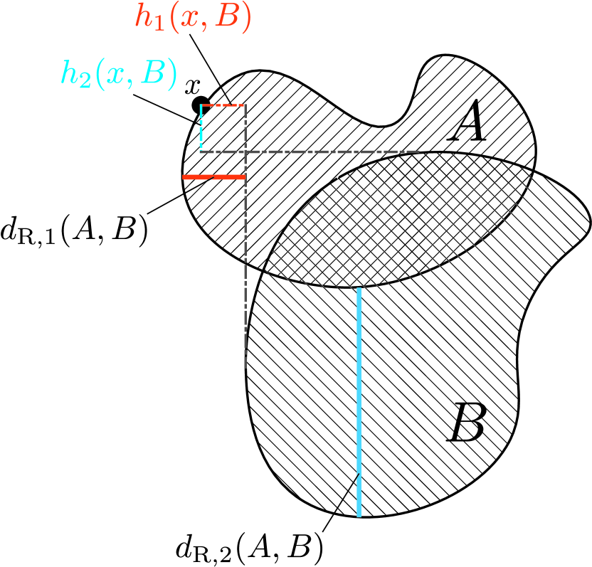
On each Cartesian axis $i=1,\ldots,n$ , consider each point $x\in A$ and $y\in B$ . We denote by $h_{i}(x,B)$ the following:

\begin{split}h_{i}(x,B)=\min\{|x_{i}-y_{i}|:y\in B\}.\end{split}

If $B=\emptyset$ , we say $h_{i}(x,B)=\infty$ .

We denote the hyperrectangular distance as $d_{\mathrm{R},i}(A,B)=\max\{\max_{x\in A}h_{i}(x,B),\max_{y\in B}h_{i}(y,A)\}$ . Combining each component, we define

d_{\mathrm{R}}(A,B):=\begin{bmatrix}d_{\mathrm{R},1}(A,B)&\cdots&d_{\mathrm{R},n}(A,B)\end{bmatrix}^{\mathsf{T}}.

Remark 2.

The value of $h_{i}(x,B)$ shown above corresponds to the shortest distance from $x$ where there exists a hyperplane on a line from $x$ in the direction of $e_{i}$ , with a normal direction $e_{i}$ , that intersects $B$ (see Fig. 1 for an illustration). If such an intersecting hyperplane does not exist, we say $h_{i}(x,B)=\infty$ . We then have $d_{\mathrm{R},i}(A,B)=\max\{\max_{x\in A}h_{i}(x,B),\max_{y\in B}h_{i}(y,A)\}$ , as shown in Fig. 1.

From Definition 4 it trivially follows that for two compact sets $A,B\subseteq\mathbb{R}^{n}$ , we have $A_{\boxplus\rho}\supseteq B$ and $B_{\boxplus\rho}\supseteq A$ if and only if $\rho\succeq d_{\text{R}}(A,B)$ . This is analogous to the fattening-based characterization of the Hausdorff distance in (3).

Before we can proceed, we must impose a number of mild conditions on the differential inclusion defined by dynamics (4) and (5), as well as the initial set of states $\mathscr{X}_{0}$ . In particular, we wish to show that the reachable set $\mathbb{X}_{t}^{\rightarrow}(F,\mathscr{X}_{0})$ is connected. This property is key in proving the main result of this work.

We first present a prerequisite lemma on the connectedness of the solution set of a differential inclusion. To this end, we require the definition of the following metric space, as well as two propositions that provide sufficient conditions for $F$ to produce solution sets with connected and compact values.

Definition 5.

Let $S$ be a function space defined as

S:=\left\{x\in C([0,\infty),\mathbb{R}^{n}):\dot{x}\in L_{\mathrm{loc}}^{1}([0,\infty),\mathbb{R}^{n})\right\},

endowed with distance metric $d_{S}$ defined as

d_{S}(x,y):=\|x(0)-y(0)\|+\sum_{k=1}^{\infty}\frac{1}{2^{k}}\frac{\int_{0}^{k}\|\dot{x}(t)-\dot{y}(t)\|\ \mathrm{d}t}{1+\int_{0}^{k}\|\dot{x}(t)-\dot{y}(t)\|\ \mathrm{d}t}.

(10)

In Definition 5, $(S,d_{S})$ is a complete metric space [21, Prop. 1, p. 1007].

Lemma 3 ([21, Thm. 1, p. 1010]).

Consider a differential inclusion

\begin{split}\dot{x}(t)&\in F(t,x(t)),\quad\text{a.e.}\ t\in[0,T],\\ x(0)&=x_{0}\in\mathbb{R}^{n},\end{split}

where $F:[0,\infty)\times\mathbb{R}^{n}\rightrightarrows\mathbb{R}^{n}$ is a compact-valued multifunction. Let $F(t,x)$ be path-connected for all $(t,x)\in\mathbb{R}^{n}\times\mathbb{R}^{n}$ , and let $F(t,x)$ be continuous and Lipschitz in $t$ and $x$ . Then for any $x_{0}\in\mathbb{R}^{n}$ , the set of solutions

\begin{split}S_{F}(x_{0}):=\{x\in S:&x(0)=x_{0},\\ &\dot{x}(t)\in F(t,x(t))\ \text{a.e.}\ t\in[0,\infty)\},\end{split}

is path-connected in the space $(S,d_{S})$ .

Remark 3.

Since the conditions of Lemma 3 on $F$ will be required throughout this work, we will look at the applicability of these conditions to commonly encountered classes of dynamical systems. We list two here:

1.

Affine-in-control systems: Consider functions $g:[0,\infty)\times\mathbb{R}^{n}\to\mathbb{R}^{n}$ and $h:[0,\infty)\times\mathbb{R}^{n}\to\mathbb{R}^{n\times m}$ that form the following differential equation:

$\dot{x}(t)=g(t,x(t))+h(t,x(t))u(t).$

From this system, we can introduce a differential inclusion defined by a multifunction

$F(t,x):=\{g(t,x)\}\oplus h(t,x)\mathscr{U},$

where $\mathscr{U}\subseteq\mathbb{R}^{m}$ is nonempty, compact, and path-connected. If $g$ and $h$ are continuous and Lipschitz in their arguments, then $F$ will satisfy conditions of Lemma 3.
2.

General nonlinear systems: For a dynamical system of the form of (4), a sufficient condition for $F(t,x):=f(t,x,\mathscr{U})$ to satisfy the condition of Lemma 3, is for $\mathscr{U}$ to be nonempty, compact, and path-connected, and $f(t,x)$ to be continuous and Lipschitz in $t$ and $x$ .

Relaxations to the conditions of Lemma 3 are presented in Appendix 6.

We proceed to prove that path-connectedness of $S_{F}(x_{0})$ implies that the values of $S_{F}^{t}(x_{0}):=\{x(t):x\in S_{F}(x_{0})\}$ are connected for all $t\in[0,\infty)$ .

Proposition 1 (Path-connectedness of $S_{F}^{t}(x_{0})$ ).

For some multifunction $F$ satisfying the hypotheses of Lemma 3, and some $x_{0}\in\mathbb{R}^{n}$ , the set $S_{F}^{t}(x_{0})=\{x(t):x\in S_{F}(x_{0})\}$ is path-connected for all $t\in[0,\infty)$ .

Proof.

We consider the case where $\#S_{F}(x_{0})>1$ ; the case of a singleton is trivial. To show that the values of $S_{F}(x_{0})$ are path-connected, let us first note that for any $x,y\in S_{F}(x_{0})$ , there exists a continuous path $p:[0,1]\to S_{F}(x_{0})$ such that $p(0)=x$ and $p(1)=y$ . For all $t$ , for any $a,b\in S_{F}(x_{0})(t)$ , there exist at least one pair of functions $(x_{a},x_{b})\subseteq S_{F}(x_{0})$ such that $x_{a}(t)=a$ , $x_{b}(t)=b$ . Let $p_{a,b}:[0,1]\to S_{F}(x_{0})$ be a path that connects $x_{a}$ and $x_{b}$ , which exists by path-connectedness of $S_{F}(x_{0})$ . Then, $p(\cdot)(t):[0,1]\to\mathbb{R}^{n}$ is a path between $a$ and $b$ . Hence, the values of $S_{F}(x_{0})(t)$ are path-connected for all $t\in[0,\infty)$ . $\square$ ∎

In Proposition 1, we have shown that the sets $S_{F}^{t}(x_{0})$ for $t\in[0,\infty)$ are path-connected. In our main theorem, we will also require that these sets are compact and nonempty. The following proposition guarantees this.

Proposition 2 ( $S_{F}^{t}(x_{0})$ forms a path-connected continuum).

For a differential inclusion

\begin{split}\dot{x}(t)&\in F(t,x(t)),\quad\text{a.e.}\ t\in[0,T],\\ x(0)&=x_{0}\in\mathbb{R}^{n},\end{split}

where $F:[0,\infty)\times\mathbb{R}^{n}\rightrightarrows\mathbb{R}^{n}$ is a compact-valued multifunction. Let $F$ satisfy the hypotheses of Lemma 3.

Then, for any $x_{0}\in\mathbb{R}^{n}$ , the solution set $S_{F}(x_{0})$ is a path-connected continuum in $S$ , i.e., a nonempty, compact, path-connected subset of $S$ . In addition, the sets $S_{F}^{t}(x_{0})$ are path-connected continua in $\mathbb{R}^{n}$ for all $t\in[0,\infty)$ .

Proof.

The fact that $S_{F}(x_{0})$ is a nonempty compact subset of $S$ follows from [22, Thm. 5.1, p. 228]. It is clear that the values of $S_{F}(x_{0})$ will be nonempty, since $\#S_{F}(x_{0})>0$ . Given some $t\in[0,\infty)$ , we define a functional $E_{t}:S\to\mathbb{R}^{n}$ as $E_{t}(x):=x(t)$ . If $E_{t}$ can be shown to be continuous, then $E_{t}$ is a preserving map in the sense of [23, p. 21], i.e., the image $E_{t}(S_{F}(x_{0}))=S_{F}^{t}(x_{0})\subseteq\mathbb{R}^{n}$ preserves the compactness and path-connectedness properties of $S_{F}(x_{0})$ . We proceed to show that $E_{t}$ is indeed a continuous linear functional.

We require linearity to show that $E_{t}$ is uniformly continuous on all of $S$ . To show that $E_{t}$ is linear, consider two functionals $x,y\in S$ , and a scalar $\alpha\in\mathbb{R}$ . We clearly find

\begin{split}E_{t}(x+y)&=(x+y)(t)=x(t)+y(t)=E_{t}(x)+E_{t}(y),\\ E_{t}(\alpha x)&=(\alpha x)(t)=\alpha x(t)=\alpha E_{t}(x).\end{split}

If $E_{t}$ is linear, by [24, Thm. 1.1, p. 54] it suffices to show that $E_{t}$ is continuous at any one $y\in S$ . Continuity of the functional is shown next by using the $\delta$ – $\epsilon$ criterion [24, p. 52].

We proceed to show that for each $\epsilon>0$ , there exists some $\epsilon^{\prime}>0$ such that $\|E_{t}(x)-E_{t}(y)\|<\epsilon$ for all $x\in S$ such that $d_{S}(x,y)<\epsilon^{\prime}$ . To this end, let us define $a_{k}:=\int_{0}^{k}\|\dot{x}(t)-\dot{y}(t)\|\ \mathrm{d}t$ . By definition of the solution set, we have for any $x,y\in S_{F}(x_{0})$ :

\begin{split}d_{S}(x,y)&=\|x(0)-y(0)\|+\sum_{k=1}^{\infty}\frac{1}{2^{k}}\frac{a_{k}}{1+a_{k}}\\ &=\sum_{k=1}^{\infty}\frac{1}{2^{k}}\frac{a_{k}}{1+a_{k}}=\sum_{k=1}^{\infty}\frac{1}{2^{k}}\frac{1}{1+a_{k}^{-1}},\end{split}

since $x(0)=y(0)=x_{0}$ .

We know by path-connectedness of $S_{F}(x_{0})$ that for any $x\in S_{F}(x_{0})$ , given some $\epsilon^{\prime}>0$ , there exists $y\in S_{F}(x_{0})\setminus\{x\}$ such that $d_{S}(x,y)<\epsilon^{\prime}$ . In general, we can upper-bound the difference between values of $x$ and $y$ at time $t$ as follows:

\begin{split}\|x(t)-y(t)\|&=\left\|x(0)+\int_{0}^{t}\dot{x}(s)\ \mathrm{d}s-y(0)-\int_{0}^{t}\dot{y}(s)\ \mathrm{d}s\right\|\\ &=\left\|\int_{0}^{t}\dot{x}(s)-\dot{y}(s)\ \mathrm{d}s\right\|\leq\int_{0}^{t}\|\dot{x}(s)-\dot{y}(s)\|\ \mathrm{d}s,\end{split}

which follows from Jensen’s inequality [25, p. 109].

Given some $\epsilon>0$ and $t\in(0,\infty)$ , let $K:=\lceil t\rceil\in\mathbb{N}$ . Since $\int_{0}^{t}\|\dot{x}(s)-\dot{y}(s)\|\ \mathrm{d}s<\epsilon$ implies $d(x(t),y(t))<\epsilon$ , it suffices to show that there exists some $\epsilon^{\prime}>0$ , such that any $y\in S_{F}(x_{0})\setminus\{x\}$ that satisfies $d_{S}(x,y)<\epsilon^{\prime}$ yields $\int_{0}^{t}\|\dot{x}(s)-\dot{y}(s)\|\ \mathrm{d}s<\epsilon$ . We choose $\epsilon^{\prime}$ as follows:

\begin{split}d_{S}(x,y)&=\sum_{k=1}^{\infty}\frac{1}{2^{k}}\frac{1}{1+a_{k}^{-1}}\\ &\geq\left(\sum_{k=1}^{K}\frac{1}{2^{k}}\frac{1}{1+\epsilon^{-1}}\right)+\left(\sum_{k=K+1}^{\infty}\frac{1}{2^{k}}\frac{1}{1+a_{k}^{-1}}\right)\\ &\geq\sum_{k=1}^{K}\frac{1}{2^{k}}\frac{1}{1+\epsilon^{-1}}=:\epsilon^{\prime}(t,\epsilon).\end{split}

We may evaluate $\epsilon^{\prime}(t,\epsilon)$ as

\epsilon^{\prime}(t,\epsilon)=\frac{(1-2^{-K})\epsilon}{1+\epsilon}>0.

If we consider $y\in S_{F}(x_{0})\setminus\{x\}$ such that $d_{S}(x,y)<\epsilon^{\prime}(t,\epsilon)$ , we have therefore shown that we obtain $d(x(t),y(t))<\epsilon$ ; at least one such $y$ exists by path-connectedness of $S_{F}(x_{0})$ . We thus proved continuity of $E_{t}$ .

Having shown that $E_{t}$ is a continuous (linear) operator (and therefore a preserving map), we have proven that $E_{t}(S_{F}(x_{0}))$ is a path-connected continuum for all $t\in[0,\infty)$ and $x_{0}\in\mathbb{R}^{n}$ . $\square$ ∎

Given the result of Proposition 2, we can now show that given the above conditions and a condition on the initial set of states, the reachable set $\mathbb{X}_{t}(F,\mathscr{X}_{0})$ is also path-connected.

Lemma 4.

For a differential inclusion

\begin{split}\dot{x}(t)&\in F(t,x(t)),\quad\text{a.e.}\ t\in[0,T],\\ x(0)&=x_{0}\in\mathbb{R}^{n},\end{split}

where $F:[0,\infty)\times\mathbb{R}^{n}\rightrightarrows\mathbb{R}^{n}$ satisfies all conditions listed in Proposition 2, given a path-connected continuum $\mathscr{X}_{0}\subseteq\mathbb{R}^{n}$ , reachable set $\mathbb{X}_{t}^{\rightarrow}(F,\mathscr{X}_{0})$ is path-connected for all $t\in[0,\infty)$ .

Proof.

We draw upon [26, Cor. 4.5, p. 233], which says that the choice of $F$ in Lemma 3 is sufficient for the solution set $S_{F}:\mathbb{R}^{n}\rightrightarrows S$ to be continuous on $\mathbb{R}^{n}$ . In other words, the solution set $S_{F}$ has a continuous dependence on the initial value.

We characterize the reachable set as follows:

R_{F}(t):=\mathbb{X}_{t}^{\rightarrow}(F,\mathscr{X}_{0})=\bigcup_{x_{0}\in\mathscr{X}_{0}}S_{F}^{t}(x_{0}),

It is clear that for any two values $a,b\in R_{F}(t)$ , there exist $x_{0},x_{0}^{\prime}\in\mathscr{X}_{0}$ such that $a\in S_{F}^{t}(x_{0})$ and $b\in S_{F}^{t}(x_{0}^{\prime})$ . Since $\mathscr{X}_{0}$ is path-connected and $S_{F}$ is continuous, there exists a continuous path $p_{0}:[0,1]\to\mathscr{X}_{0}$ connecting $x_{0}$ and $x_{0}^{\prime}$ . Therefore, the solution sets for $S_{F}(x_{0})$ and $S_{F}(x_{0}^{\prime})$ are connected by a path $p_{s}=S_{F}\ \circ\ p_{0}:[0,1]\rightrightarrows S$ . Since $S_{F}^{\prime}(x_{0},x_{0}^{\prime}):=\bigcup_{\tau\in[0,1]}p_{s}(\tau)$ is path-connected, this implies that its values are also path-connected, analogous to the latter part of the proof of Proposition 1. Hence, $R_{F}(t)$ is path-connected for all $t\in[0,\infty)$ . $\square$ ∎

We can now provide a means of inner and outer approximating the off-nominal reachable set based on a hyperrectangular trajectory deviation growth bound.

Theorem 2 (General FRS inner approximation with changed dynamics).

Let $f:[0,\infty)\times\mathbb{R}^{n}\times\mathscr{U}\to\mathbb{R}^{n}$ , $g:[0,\infty)\times\mathbb{R}^{n}\times\mathscr{V}\to\mathbb{R}^{n}$ , where $\mathscr{U},\mathscr{V}\subseteq\mathbb{R}^{m}$ are such that $d_{\mathrm{R}}(\mathscr{U},\mathscr{V})\preceq\epsilon$ . Let $G(t,x)=g(t,x,\mathscr{V})$ and $F(t,x)=f(t,x,\mathscr{U})$ , and let $\mathscr{X}_{0}\subseteq\mathbb{R}^{n}$ , the set of initial states, and initial time $t_{0}\in\mathbb{R}_{+}$ be given. Let $\mathscr{X}_{0}$ , $f,g$ , and $\mathscr{U},\mathscr{V}$ satisfy the conditions of Lemma 4. Let the hypotheses of Lemma 2 be satisfied with $\bar{\mathscr{U}}=\mathscr{V}$ , $t_{\mathrm{init}}=t_{0}$ , and $t_{f}>t_{\mathrm{init}}$ . Let $\eta(t,\epsilon)$ be obtained as in Lemma 2. Then:

(i)

For each $x_{0}\in\mathscr{X}_{0}$ there exists a trajectory $x(t)$ emanating from $x(t_{0})=x_{0}$ with $\dot{x}(t)\in F(t,x(t))$ and a trajectory $y(t)$ satisfying $y(t_{0})=x_{0}$ and $\dot{y}(t)\in G(t,y(t))$ such that $|x(t)-y(t)|\preceq\eta(t,\epsilon)$ for all $t\in[t_{0},t_{f}]$ ;
(ii)

Let $T\in[0,t_{f}-t_{0}]$ , and let $\eta^{*}=\eta(t_{0}+T,\epsilon)$ . For all $t\in[t_{0},t_{0}+T]$ , $d_{\mathrm{R}}[\mathbb{X}^{\rightarrow}_{t}(G,\mathscr{X}_{0}),\mathbb{X}^{\rightarrow}_{t}(F,\mathscr{X}_{0})]\preceq\eta^{*}$ ;

(iii)

For all $t\in[t_{0},t_{0}+T]$ ,

\mathbb{X}^{\rightarrow}_{t}(F,\mathscr{X}_{0})\setminus(\partial\mathbb{X}^{\rightarrow}_{t}(F,\mathscr{X}_{0}))_{\boxplus\eta^{*}}\subseteq\mathbb{X}^{\rightarrow}_{t}(G,\mathscr{X}_{0}).

Proof.

(i)

This fact follows directly from Lemma 2.
(ii)

From (i), the maximal distance between two points in $\mathbb{X}_{t}^{\rightarrow}(F,\mathscr{X}_{0})$ and $\mathbb{X}_{t}^{\rightarrow}(G,\mathscr{X}_{0})$ is upper-bounded by $\eta(t,\epsilon)$ . In Theorem 1 it was shown that $\eta(t,\epsilon)$ is increasing in $t$ , meaning that the hyperrectangular distance bound holds for all times $t\leq t_{0}+T$ .

(iii)

We define $A=\mathbb{X}^{\rightarrow}_{t}(G,\mathscr{X}_{0})$ and $B=\mathbb{X}^{\rightarrow}_{t}(F,\mathscr{X}_{0})$ for any $t\in[t_{0},t_{0}+T]$ . Note that in this proof, unlike in [16], $A$ and $B$ need not be convex, making the proof more technically challenging. We wish to show that $C:=B\setminus(\partial B)_{\boxplus\eta^{*}}$ is a subset of $A$ .

The inclusion $C\subseteq A$ can equivalently be shown by demonstrating that for all $x\in B\setminus A$ , we have $x\in(\partial B)_{\boxplus\eta^{*}}$ ; we prove the latter claim by contradiction. Assume that there indeed exists $x\in B\setminus A$ such that $x\not\in(\partial B)_{\boxplus\eta^{*}}$ . This point then will have some $i\in\{1,\ldots,n\}$ , such that have $d_{i}(x,\partial B):=\min\{|x_{i}-y_{i}|:y\in\partial B\}>\eta_{i}^{*}$ . From the characterization of $\eta^{*}$ in Lemma 2 and the definition of the hyperrectangular distance in Definition 4, we have $d_{\text{R}}(A,B)\leq\eta^{*}$ . In light of the contradiction given above, this inequality would then necessarily yield the following equivalent contradiction:

\begin{split}d_{i}(x,\partial B)>\max\{&\max_{x^{\prime}\in A}\min\{|x_{i}^{\prime}-y_{i}|:y\in B\},\\ &\max_{x^{\prime}\in B}\min\{|x_{i}^{\prime}-y_{i}|:y\in A\}\},\end{split}

(11)

which implies

\min\{|x_{i}-y_{i}|:y\in\partial B\}>\max_{x^{\prime}\in\partial B}\min\{|x_{i}^{\prime}-y_{i}|:y\in A\}.

Let $y^{*}\in\partial B$ be such that $d_{i}(x,y^{*})=\min\{|x_{i}-y_{i}|:y\in\partial B\}$ . By the hypotheses, in particular the compactness of $B$ , there exists some $x^{*}\in A$ such that $|x^{*}-y^{*}|\preceq\eta^{*}$ .

We identify two cases: a) $x\in\partial B\cap(B\setminus A)$ , and b) $x\in B\setminus(A\cup\partial B)$ . In case a), we find $d_{i}(x,\partial B)=0$ , which produces the desired contradiction.

We now consider case b). Let us denote by $X_{i}$ the projection of all points of a set $X\subseteq\mathbb{R}^{n}$ onto the $i$ -th Cartesian axis, such that $X_{i}\subseteq\mathbb{R}$ . Since $A$ and $B$ are both compact, connected, and nonempty, we find that $A_{i}$ and $B_{i}$ are closed intervals in $\mathbb{R}$ for each $i=1,\ldots,n$ . This fact follows trivially by considering that the projection operation is continuous, and continuous maps are preserving maps in the sense of [23, p. 21], i.e., their images preserve connectedness and compactness. From [27, Thm. 12.8, p. 116], any connected subspace of $\mathbb{R}$ is an interval, which shows that the $A_{i},B_{i}$ are compact (or closed) intervals.

We can then note that for any $y_{i}^{*}$ , there exists some $x^{*}\in A$ such that $|x_{i}^{*}-y_{i}^{*}|\leq\eta^{*}_{i}$ by Lemma 2. Finally, let $y_{i}\in\partial B_{i}$ be the other point in the boundary of the interval $B_{i}$ such that $y_{i}\neq y_{i}^{*}$ .

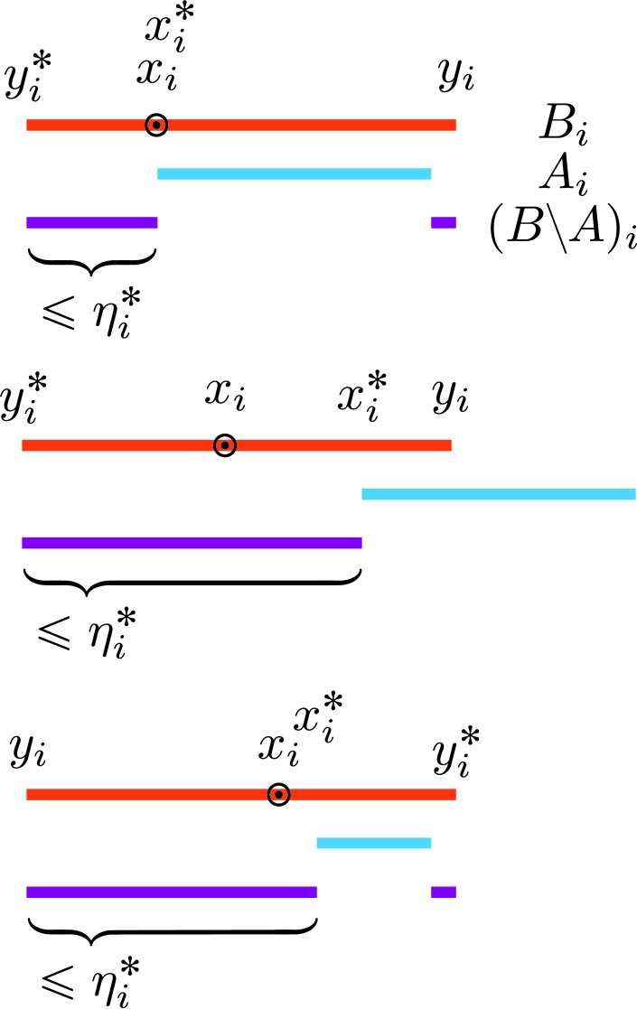
We can identify twelve arrangements of $(x,x^{*},y,y^{*})$ , barring cases of symmetry. Some of these arrangements are inadmissible, as shown below. In what follows, we must have $y^{*}\neq y$ , since $x$ would otherwise be on the boundary of $B$ , which was treated as case a). Also, necessarily, $x\neq x^{*}$ , since we have $x\not\in A$ . We prove that for each admissible arrangement, the claim of (11) does not hold; an illustration of some of these arrangements in given in Fig. 2. For some $a,b,c,d\in\mathbb{R}$ , we will denote the ordering $a<b<c<d$ by the shorthand notation $a,b,c,d$ . We have:

(a)

$x_{i}^{*},x_{i},y_{i}^{*},y_{i}$ : Not admissible since $x\not\in B\setminus A$ .
(b)

$x_{i}^{*},x_{i},y_{i},y_{i}^{*}$ ; Not admissible since $x\not\in B\setminus A$ , and inconsistent with the definition of $y^{*}$ .
(c)

$x_{i}^{*},y_{i}^{*},x_{i},y_{i}$ : In this case, by Lemma 2 we have $d(x_{i}^{*},y_{i}^{*})\leq\eta^{*}_{i}$ . Since we have $d(x_{i},y_{i}^{*})<d(x_{i}^{*},y_{i}^{*})$ , we find that $d(x_{i},y_{i}^{*})<\eta^{*}_{i}$ .
(d)

$x_{i}^{*},y_{i}^{*},y_{i},x_{i}$ : Not admissible since $x\not\in B\setminus A$ .
(e)

$x_{i}^{*},y_{i},x_{i},y_{i}^{*}$ : We have $d(x_{i}^{*},y_{i}^{*})\leq\eta^{*}_{i}$ and $d(x_{i},y_{i}^{*})<d(x_{i}^{*},y_{i}^{*})$ , which implies $d(x_{i},y_{i}^{*})<\eta^{*}_{i}$ .
(f)

$x_{i}^{*},y_{i},y_{i}^{*},x_{i}$ : Not admissible since $x\not\in B\setminus A$ .
(g)

$x_{i},x_{i}^{*},y_{i}^{*},y_{i}$ : Not admissible since $x\not\in B\setminus A$ .
(h)

$x_{i},x_{i}^{*},y_{i},y_{i}^{*}$ : Not admissible since $x\not\in B\setminus A$ , and not consistent with the definition of $y^{*}$ .
(i)

$x_{i},y_{i}^{*},x_{i}^{*},y_{i}$ : Not admissible since $x\not\in B\setminus A$ .
(j)

$x_{i},y_{i},x_{i}^{*},y_{i}^{*}$ : Not admissible since $x\not\in B\setminus A$ , and inconsistent with the definition of $y^{*}$ .
(k)

$y_{i}^{*},x_{i}^{*},x_{i},y_{i}$ : We have $d(x_{i},y_{i})\geq d(x_{i},y_{i}^{*})$ , $d(x_{i}^{*},y_{i})>d(x_{i},y_{i})$ , as well as $d(x_{i}^{*},y_{i})\leq\eta^{*}_{i}$ . From this it follows that $d(x_{i},y_{i}^{*})<\eta^{*}_{i}$ .
(l)

$y_{i}^{*},x_{i},x_{i}^{*},y_{i}$ : We have $d(x_{i},y_{i}^{*})<d(x_{i}^{*},y_{i}^{*})\leq\eta^{*}_{i}$ .

Having considered all cases, in all admissible scenarios it follows that the statement in (11) is false. This in turn contradicts the claim that there exists $x\in B\setminus A$ such that $x\not\in(\partial B)_{\boxplus\eta^{*}}$ . Therefore, we have proven that $C\subseteq A$ .

$\square$ ∎

We now present two corollaries that cover the case of a changed set of initial conditions, as well as guaranteed overapproximations of the reachable set.

Corollary 3.

Let the hypotheses of Theorem 2 hold. In addition, let there be an off-nominal set of initial conditions $\bar{\mathscr{X}}_{0}$ that is nonempty, closed, and connected, such that $d_{\text{H}}(\mathscr{X}_{0},\bar{\mathscr{X}}_{0})\leq\kappa$ . Define $\eta(t,\epsilon,\kappa)$ as in Corollary 2. Then:

(i)

For each $x_{0}\in\mathscr{X}_{0}$ there exists a trajectory $x(t)$ emanating from $x(t_{0})=x_{0}$ with $\dot{x}(t)\in F(t,x(t))$ and a trajectory $y(t)$ satisfying $y(t_{0})=x_{0}^{\prime}$ , for some $x_{0}^{\prime}\in\{x_{0}\}_{+\kappa}\cap\bar{\mathscr{X}}_{0}$ , and $\dot{y}(t)\in G(t,y(t))$ such that $|x(t)-y(t)|\preceq\eta(t,\epsilon,\kappa)$ for all $t\in[t_{0},t_{f}]$ ;
(ii)

Let $T\in[0,t_{f}-t_{0}]$ , and let $\eta^{**}=\eta(t_{0}+T,\epsilon,\kappa)$ . For all $t\in[t_{0},t_{0}+T]$ , $d_{\mathrm{R}}[\mathbb{X}^{\rightarrow}_{t}(G,\bar{\mathscr{X}}_{0}),\mathbb{X}^{\rightarrow}_{t}(F,\mathscr{X}_{0})]\preceq\eta^{**}$ ;

(iii)

For all $t\in[t_{0},t_{0}+T]$ ,

\mathbb{X}^{\rightarrow}_{t}(F,\mathscr{X}_{0})\setminus(\partial\mathbb{X}^{\rightarrow}_{t}(F,\mathscr{X}_{0}))_{\boxplus\eta^{**}}\subseteq\mathbb{X}^{\rightarrow}_{t}(G,\bar{\mathscr{X}}_{0}).

Proof.

The proof immediately follows by consideration of Corollary 2. $\square$ ∎

Corollary 4.

Let the hypotheses of Theorem 2 and Corollary 3 hold. Then:

(i)

For each $x_{0}\in\mathscr{X}_{0}$ there exists a trajectory $x(t)$ emanating from $x(t_{0})=x_{0}$ with $\dot{x}(t)\in F(t,x(t))$ , and a trajectory $y(t)$ satisfying $y(t_{0})=y_{0}$ with $y_{0}\in\bar{\mathscr{X}}_{0}$ such that $\|x_{0}-y_{0}\|\leq\kappa$ and $\dot{y}(t)\in G(t,y(t))$ , such that $|x(t)-y(t)|\preceq\eta(t,2\delta+\epsilon,\kappa)$ for all $t\in[t_{0},t_{f}]$ and $i=1,\ldots,n$ , where $\delta:=\max_{u\in\mathscr{U}}\|u\|$ ;
(ii)

For all $t\in[t_{0},t_{f}]$ , $d_{\mathrm{R}}[\mathbb{X}^{\rightarrow}_{t}(G,\bar{\mathscr{X}}_{0}),\mathbb{X}^{\rightarrow}_{t}(F,\mathscr{X}_{0})]\preceq\eta(t_{f},2\delta+\epsilon,\kappa)$ ;

(iii)

For all $t\in[t_{0},t_{f}]$ ,

\mathbb{X}^{\rightarrow}_{t}(G,\bar{\mathscr{X}}_{0})\subseteq(\mathbb{X}^{\rightarrow}_{t}(F,\mathscr{X}_{0}))_{\boxplus\eta(t_{f},2\delta+\epsilon,\kappa)}.

Proof.

(i)

This claim follows from Lemma 1, where we have used the following inequality:

\|u(t)-v(t)\|\leq\|u(t)\|+\|v(t)\|\leq\delta+\delta+d_{\mathrm{H}}(\mathscr{U},\mathscr{V})\leq 2\delta+\epsilon,

which follows from the triangle inequality, as well as the definition of the Hausdorff distance.

(ii)

This fact follows directly from Lemma 1.
(iii)

The proof here is similar to that of Theorem 2(iii), where we consider that any point in $A$ has a counterpart in $B$ that is distance $\eta(t_{f},2\delta+\epsilon)$ away. The proof is immediate from this consideration and Lemma 2.

$\square$ ∎

Remark 4.

In Corollaries 3 and 4, the Hausdorff distance upper bound $\kappa$ on the initial set of states does not decrease the quality of the inner approximation with increasing time, similar to the quantity $2\delta+\epsilon$ . In fact, the approximations decrease in tightness with increasing time solely on account of the ‘looseness’ of the functions $\tilde{a},\tilde{b},\tilde{w}$ of Lemma 2 that upper-bound the trajectory deviation growth.

4 Simulation results

We consider three numerical examples: a simplified representation of the heading dynamics of a sea-faring vessel, and lower triangular dynamical system, and an interconnected system of linear subsystems. The restriction to lower dimension systems stems from computational limitations in obtaining the nominal reachable sets with sufficient accuracy, as well as a desire to keep derivations concise. We will show how Theorem 2 and Corollary 4 can be applied to these systems. For both examples, we have used the CORA MATLAB toolkit [28] to compute the nominal and off-nominal reachable sets for illustrative purposes; in reality, such tools are not required to apply the theory presented here. In practice, the nominal reachable set would be computed prior to the system’s operation using a similar toolkit. The methods used in such toolkits can often not be used online because of hardware limitations and poor scalability, hence the need for an approach such as ours.

In practice, it is difficult to obtain a hyperrectangular slimming of the form $X\setminus(\partial X)_{\boxplus\rho}$ using widely used software packages. For this reason, we propose an alternative using a conservative ball-based slimming operation. It is obvious that the following holds:

X\setminus(\partial X)_{+\|\rho\|}\subseteq X\setminus(\partial X)_{\boxplus\rho},

(12)

where $\|\rho\|$ denotes the Euclidean norm of the vector $\rho$ . This follows from the fact that the ball $\mathcal{B}_{+\|\rho\|}$ includes the hyperrectangle $\operatorname*{\scalerel*{\times}{\sum}}_{i=1}^{n}[-\rho_{i},\rho_{i}]$ . In the following, we will show approximations based on naive ball-based slimming using single elements $\rho$ , which give an indication of the shape of a true hyperrectangular slimming in that particular dimension. We also give a guaranteed inner approximation by applying a ball-based slimming operation with radius $\|\rho\|$ .

Compared to [16], this approximation approach yields tighter approximations, since the bounds obtained there are greater or equal to $\|\rho\|$ , as a bound on the Euclidean norm of the trajectory deviation is used there.

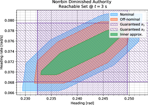
4.1 Norrbin’s Ship Steering Dynamics

We first consider Norrbin’s model of the heading dynamics of a ship sailing at constant velocity [29]:

\dot{x}(t)=\begin{bmatrix}\dot{x}_{1}(t)\\ \dot{x}_{2}(t)\end{bmatrix}=f(x(t),u(t))=\begin{bmatrix}x_{2}\\ -\frac{v}{2l}(x_{2}+x_{2}^{3})\end{bmatrix}+\begin{bmatrix}0\\ \frac{v^{2}}{2l^{2}}\end{bmatrix}u,

where $x_{1}$ is the heading (or yaw) angle, and $x_{2}$ is the heading rate; in this example, $u$ denotes the rudder angle, $v$ denotes the fixed cruise speed, and $l$ denotes the vessel length. As can be observed in the dynamics, a vessel’s ability to make turns is strongly correlated with its velocity (higher speeds provide greater resistance, but induce stronger rudder authority), as well as the length of the vessel. Intuitively, a longer vessel is harder to turn due to its inertia and hydrodynamic resistance of the hull. The dynamics are of second order, as a rudder deflection naturally induces a yaw moment.

We can find the following bound on trajectory deviation growth:

\begin{split}&|\tilde{f}(\bar{x},\bar{u})|=|f(x+\tilde{x},u+\tilde{u})-f(x,u)|\\ &\preceq\begin{bmatrix}|\tilde{x}_{2}|\\ \frac{v}{2l}(|\tilde{x}_{2}|+|\tilde{x}_{2}|^{3}+3|\tilde{x}_{2}|^{2}|M_{2}|+3|\tilde{x}_{2}||M_{2}|^{2})+\frac{v^{2}}{2l^{2}}|\tilde{u}|\end{bmatrix},\end{split}

(13)

where $M_{2}=\max_{y\in\mathbb{X}_{t}^{\rightarrow}(F,\mathscr{X}_{0})}|y_{2}|$ . $M_{2}$ can be determined since the nominal reachable set $\mathbb{X}_{t}^{\rightarrow}(F,\mathscr{X}_{0})$ is available to us. We note that (13) contains an integrator in state $\tilde{x}_{1}$ , which allows us to obtain a hyperrectangular trajectory deviation bound as follows. We first compute the deviation bound on state $\tilde{x}_{2}$ , such that $|\tilde{x}_{2}(t)|\leq\eta_{2}(t)$ . We then compute an upper bound on $\tilde{x}_{1}$ , which is of the form $\eta_{1}(t)=\int_{t_{0}}^{t}\eta_{2}(\tau)\ \text{d}\tau$ , which gives $|\tilde{x}_{1}(t)|\leq\eta_{1}(t)$ . Alternatively, a more conservative expression for $\eta_{1}$ can be obtained by defining it as $\eta_{1}(t):=\eta(t_{f})t$ , which follows from the fact that $\eta$ is strictly increasing (see the proof of Theorem 1).

4.1.1 Diminished Control Authority

In this example, we define multifunction $F$ as $F(x):=f(x,\mathscr{U})$ , with $\mathscr{U}=[-25^{\circ},25^{\circ}]$ and the impaired control set is $\bar{\mathscr{U}}=[-20^{\circ},20^{\circ}]$ , hence $\epsilon=d_{\mathrm{H}}(\mathscr{U},\bar{\mathscr{U}})=5^{\circ}$ . We consider the initial set of states to be a singleton: $\mathscr{X}_{0}=\{[\begin{smallmatrix}0^{\circ}&5^{\circ}/\text{s}\end{smallmatrix}]^{\mathsf{T}}\}$ . The nominal velocity is taken as $v=5$ m/s, and the length of the vessel is $l=45$ m.

We first consider the case of diminished control authority, i.e., the case in which the system dynamics remain the same, but the control inputs are draw from $\bar{\mathscr{U}}$ instead of $\mathscr{U}$ .

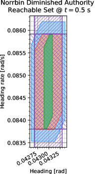
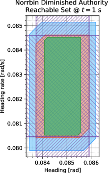
We evaluate the reachable set at $t=0.5$ s, $t=1$ s, and $t=3$ s, yielding the results shown in Fig. 3. We have given a guaranteed inner approximation based on the conservative ball-based slimming approach, as well as guaranteed intervals in each Cartesian axis using the entries of $\eta(t)$ . These guaranteed intervals are shown as cross-hatched areas, and give an indication of what a hyperrectangular slimming would have produced, in addition to providing a guarantee that there exists at least one state in the off-nominal reachable set that has one of its coordinates on one of the intervals. Unlike the results in [16], the quality of the inner approximations degrades little with time (see Fig. 3(c)). This feature can be attributed to the fact that we are using a hyperrectangular growth bound in this work, as opposed to a more conservative norm-based bound.

An application to computing a guaranteed reachable set of the positions of the ship after control authority diminishment based on Norrbin’s model has been prepared as a video¹¹1Demonstration of the computation of a guaranteed reachable set for the Norrbin ship model under diminished rudder authority: https://youtu.be/5eUINOGJ_0Y.

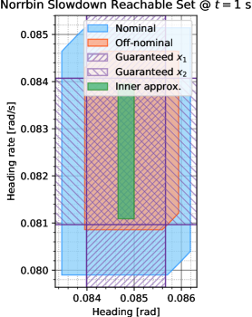
4.1.2 Changed Dynamics

In addition to the diminished control authority, we now also consider the following changed dynamics:

\dot{x}(t)=g(x(t),u(t))=\begin{bmatrix}x_{2}\\ -\frac{v_{\text{s}}}{2l}(x_{2}+x_{2}^{3})\end{bmatrix}+\begin{bmatrix}0\\ \frac{v_{\text{s}}^{2}}{2l^{2}}\end{bmatrix}u,

where we consider $v_{s}<v$ and $v_{s}>v$ , to capture a slowdown and speedup of the vessel, respectively.

Slowdown

We first consider $v_{\text{s}}=0.95v=4.75$ m/s. This slowdown causes the reachable set to shrink and shift slightly towards higher heading angles, since there is insufficient velocity to reach lower angles. The bound given in Lemma 1 is used, where we define $\gamma(t)$ as follows:

\gamma(t):=\frac{|v_{\text{s}}-v|}{2l}(m_{2}+m_{2}^{3})+\frac{v^{2}-v_{\text{s}}^{2}}{2l^{2}}\max_{u\in\mathscr{U}}|u|,

where $m_{2}=\min_{y\in\mathbb{X}_{t}^{\rightarrow}(F,\mathscr{X}_{0})}y_{2}$ . Combining this bound with the trajectory deviation growth bound given at the beginning of this section, we obtain the conservative inner approximation shown in Fig. 4. As can be clearly seen, not only is the off-nominal reachable set smaller, but it has also drifted to the top-left. This change is intuitively correct, since at a slower velocity rudder inputs become more effective as the vessel can make tighter turns at slower speeds. This phenomenon is reflected in the upward shift in heading rate and heading angle. A large area of the actual off-nominal set is lost due to the need for coping with

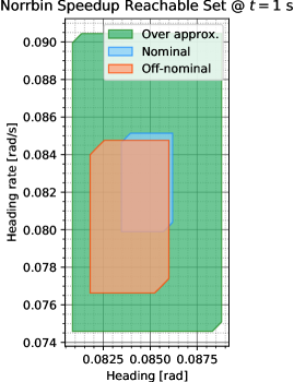
Speedup

We now demonstrate outer approximations in the case of changed dynamics. We still consider a diminishment in control authority, but in this case, $v_{\text{s}}=1.4v=7$ m/s, indicating a speedup. In practice, one would like to know what the worst case trajectory could be in such a case, for example when attempting to avoid a high speed vessel. Instead of shrinking the nominal set, we now fatten it as shown in Corollary 4. Our $\gamma(t)$ in this setting is as follows:

\gamma(t):=\frac{v_{\text{s}}-v}{2l}(M_{2}+M_{2}^{3})+\frac{|v^{2}-v_{\text{s}}^{2}|}{2l^{2}}\max_{u\in\mathscr{U}}|u|.

With a similar trajectory deviation growth bound as in the case of a slowdown, we obtain an outer approximation as shown in Fig. 5, this time with an exact hyperrectangular fattening. In this case, it is also possible to apply a conservative ball-based fattening using the same radius as given previously.

In Fig. 5, it is clear that the off-nominal reachable set has shifted towards lower heading angles as rates, since the vessel will have less effective rudder authority at higher cruise speeds due to the its inertia. As a result, the outer approximation includes a large area of unused space towards the top right, since it needs to make up for both the translation and growth of the off-nominal reachable set with respect to the nominal reachable set.

4.2 Cascaded System

To demonstrate that the approach given in Theorem 2 is scalable for high-dimensional systems, we present the following academic example. We consider a lower triangular system; such systems often arise in practice when dealing with interconnected dynamical systems [30]. Namely, we consider the system:

\dot{x}(t)=\begin{bmatrix}\dot{x}_{1}(t)&\cdots&\dot{x}_{n}(t)\end{bmatrix}^{\mathsf{T}}=Ax(t)+Bu(t)+d(t),

(14)

where $x\in\mathbb{R}^{n}$ and $u\in\mathscr{U}\subseteq\mathbb{R}^{m}$ , $A\in\mathbb{R}^{n\times n}$ is a lower triangular matrix, $B\in\mathbb{R}^{n\times m}$ is arbitrary, and $d:[t_{0},\infty)\to\mathbb{R}^{n}$ is a differentiable function. The contribution of $d(t)$ is that of a nonlinear drift, possibly due to phenomena such as actuator bias or periodic disturbances.

We consider both the case of diminished control authority and changed dynamics below.

4.2.1 Diminished Control Authority

We consider an off-nominal set of admissible control inputs $\bar{\mathscr{U}}\subseteq\mathscr{U}$ such that $d_{\text{H}}(\mathscr{U},\bar{\mathscr{U}})\leq\epsilon$ . Let $\dot{\tilde{x}}(t)=x(t)-\bar{x}(t)=A\tilde{x}(t)+B\tilde{u}(t)$ , where $x(t)$ is a solution of the nominal system, and $\bar{x}(t)$ corresponds to the off-nominal system. It is then straightforward to show that a hyperrectangular trajectory deviation bound can be computed as follows:

|\dot{\tilde{x}}_{i}(t)|\leq\sum_{j=1}^{i-1}|a_{i,j}|\rho_{j}(t)+|a_{i,i}||\tilde{x}_{i}(t)|+\sum_{j=1}^{m}|b_{i,j}|\epsilon,

(15)

where each $\rho_{j}(t)$ is computed as per Lemma 2. We will now show how to obtain the hyperrectangular trajectory deviation bound. Given the lower triangular structure of matrix $A$ , by (15) we first compute $\rho_{1}(t)$ from the following growth bound:

|\dot{\tilde{x}}_{1}(t)|\leq|a_{1,1}||\tilde{x}_{1}(t)|+\sum_{j=1}^{m}|b_{1,j}|\epsilon.

By an application of Lemma 1, we can obtain $\rho_{1}(t)$ . Repeated application of (15) and Lemma 1 will then yield the hyperrectangular deviation bound $\rho(t)$ .

4.2.2 Changed Dynamics

Let us now consider the case where $d(t)$ in (14) is replaced by $\bar{d}(t)$ , such that $|d_{i}(t)-\bar{d}_{i}(t)|\leq\gamma_{i}(t)$ . Let $\dot{\tilde{x}}(t)=x(t)-\bar{x}(t)=A\tilde{x}(t)+B\tilde{u}(t)+d(t)-\bar{d}(t)$ , where $x(t)$ is a solution of the nominal system, and $\bar{x}(t)$ corresponds to the off-nominal system. It then suffices to modify (15) as follows:

|\dot{\tilde{x}}_{i}(t)|\leq\sum_{j=1}^{i-1}|a_{i,j}|\rho_{j}(t)+|a_{i,i}||\tilde{x}_{i}(t)|+\sum_{j=1}^{m}|b_{i,j}|\epsilon+\gamma_{i}(t),

(16)

which is obtained by the same arguments as in Lemma 1.

As an illustration of the bound given in (15), we consider the following parameters:

\begin{split}A_{i,j}&=\begin{cases}j/i,\quad&j\leq i\\ 0,\quad&j>i\end{cases},\quad B_{i,j}=j/(9-i),\quad d_{i}(t)=0.1\end{split}

We take the admissible set of control inputs to be $\mathscr{U}=\operatorname*{\scalerel*{\times}{\sum}}_{i=1}^{n}[-1,1]$ , and the diminished set of control inputs is $\bar{\mathscr{U}}=\operatorname*{\scalerel*{\times}{\sum}}_{i=1}^{m}[-0.9,0.9]$ , so that $\epsilon=d_{\mathrm{H}}(\mathscr{U},\bar{\mathscr{U}})=0.1$ . We take $n=5$ , and $m=8$ . By applying the bound on the trajectory deviation growth given in (16), we can compute inner-approximations to the impaired reachable set as per Theorem 2. We consider here a final time of $t=0.25$ , and an initial set of states $\mathscr{X}_{0}=\{0\}$ . The results are given as length fractions of the projections in Table 1. Using the notation of Theorem 2, for each $i$ -th Cartesian dimension, the first column gives the ratio

\mathrm{length}[B_{i}\setminus((\partial B)_{i})_{+\rho_{i}(t)}]/\mathrm{length}[A_{i}],

and the second column shows

\mathrm{length}[B_{i}\setminus((\partial B)_{i})_{+\|\rho(t)\|}]/\mathrm{length}[A_{i}].

It can clearly be observed that the volume fractions of the inner approximations remain reasonably tight with increasing system dimension when considering the tightness of the hyperrectangular distance bound. These results serve to demonstrate that our method is capable of producing reasonably tight approximations even for systems with increased dimension by exploiting partially decoupled system structure. In comparison, ball-based slimming used in [16] yields worse results, as can be seen by comparing the fourth and fifth column of Table 1. For instance, a hyperrectangular shrinking operations defined by $\eta=[\begin{smallmatrix}0.1&10\end{smallmatrix}]^{\mathsf{T}}$ yields a sufficient ball-based shrinking operation with radius $\|\eta\|\approx 10$ , which would likely shrink away most of the first Cartesian dimension in practice. A similar phenomenon can be observed when considering dimensions 1 and 3 in Table 1; using hyperrectangular bounds prevents excessive slimming of the reachable set.

Table 1: Projected length ratios of the lower triangular system example by dimension using hyperrectangular and ball-based slimming operations.

Dim.	Hyperrect. inner-approx./Off-nominal length	Ball-based inner-approx./Off-nominal length
1	88.3%	29.8%
2	87.7%	41.7%
3	87.0%	52.8%
4	63.8%	18.8%
5	58.0%	30.3%

4.2.3 Computational Complexity

To show that the theory presented in this work is scalable on systems such as (14), we consider the computational complexity of a basic algorithmic implementation to compute $\rho_{i}$ for each $i$ , as well as verifying if a state is guaranteed to lie in the off-nominal reachable set. Both of these tasks are subject to hard real-time constraints in practice, making it essential to study how their computational complexity grows.

Computing the Trajectory Deviation Bound

We note that we must perform numerical integration to compute $G$ , $\int a(\tau)\ \textrm{d}\tau$ , and $\int b(\tau)\ \textrm{d}\tau$ in the Bihari inequality (7). To compute the inverse $G^{-1}$ , one may use a root-finding scheme or an approximate look-up table (LUT) based approach. We consider here a LUT approach.

When using a method an explicit non-adaptive numerical integration scheme such as Euler’s method or Runge-Kutta, it suffices to consider an a priori set integration step $h>0$ . Let us consider the reachable set in an interval $t\in[0,T]$ , and take $h=T/N$ with $N\in\mathbb{N}$ . By the results from [31], the computational complexity of a Runge-Kutta scheme is $\mathcal{O}(N)$ . Since we will need to perform three rounds of numerical integration per dimension (for $G$ , and in $a$ and $b$ ), which together take $\mathcal{O}(N)$ . We store all value of $G$ and their argument $r$ in a lookup table of size $N$ . Since values can be retrieved from an array in constant time, the complexity of numerical integration to populate the LUT combined with lookup is $\mathcal{O}(1)+\mathcal{O}(N)=\mathcal{O}(N)$ . We then note that this process must be repeated for all $n$ dimensions, which gives computational complexity $\mathcal{O}(nN)$ . Therefore, the value of $\rho(t)$ , which is instrumental in producing guaranteed inner- and outer-approximations, can be computed in linear time with respect to the system dimension $n$ .

Verifying Reachability of a State

We now consider the complexity of verifying whether a state lies in the computed inner approximation of the reachable set. Let us assume that we have access to a signed distance function, $\psi:\mathbb{R}^{n}\to\mathbb{R}$ , of the nominal reachable set at time $t$ (see, e.g., [32, p. 811] for more information on signed distance functions). We assume that we can evaluate $\psi$ using $N_{\psi}$ primitive operations. Then, to evaluate whether or not a point $x\in\mathbb{R}^{n}$ lies in the inner approximation of the off-nominal reachable set, it suffices to check the following:

1.

Check if $\psi(x)\leq 0$ ; we must first check if $x$ lies in the nominal reachable set. If this is false, $x$ is not guaranteed to lie in the off-nominal reachable set.
2.
Check if $\psi(x)\leq-\min_{i}\rho_{i}(t)$ ; we must verify that $x$ lies at least distance $\min_{i}\rho_{i}(t)$ away from the boundary of the nominal reachable set. If this is false, $x$ is not guaranteed to lie in the off-nominal reachable set.
1. (a)
  
  Check if $\psi(x)\leq-\|\rho(t)\|$ . This verification is based on the ball-based slimming operation of (12). If this is true, $x$ is guaranteed to lie in the off-nominal reachable set. If false, continue to the next step.
2. (b)
  
  Perform gradient ascent on $\psi$ starting at $x$ , such that we reach $x^{\prime}$ that satisfies $\psi(x^{\prime})=0$ . This $x^{\prime}$ is the point on the boundary of the nominal reachable set that is closest to $x$ . Verify whether $\rho(t)\preceq|x-x^{\prime}|$ . If this inequality is true, $x$ is guaranteed to lie in the off-nominal reachable set.

In the above algorithm, it will take at least one evaluation of $\psi$ to verify whether $x$ is guaranteed to be in the off-nominal reachable set. Doing so requires $N_{\psi}$ operations, and corresponds to step 1). An evaluation of $\rho(t)$ will cost $\mathcal{O}(n)$ operations as discussed previously, which yields a complexity of $\mathcal{O}(nN_{\psi})$ . Evaluating the norm of $\rho(t)$ can be done in linear time as part of step 2a), but performing gradient ascent in step 2b) may require a significant number of evaluations of $\psi$ . It is possible to truncate the gradient ascent algorithm based on a maximum number of evaluations of $\psi$ , say $N_{\mathrm{eval}}$ . Given some $x^{\prime\prime}\in\mathbb{R}^{n}$ obtained after $N_{\mathrm{eval}}-1$ evaluations of $\psi$ , it is clear that $x^{\prime}\in\{x^{\prime\prime}\}_{+|\psi(x^{\prime\prime})|}$ . We can check if for each $i=1,\ldots,n$ , it holds that $|x_{i}-x_{i}^{\prime\prime}|+|\psi(x^{\prime\prime})|\leq\rho_{i}(t)$ . If this inequality is true, then $x$ is guaranteed to lie in the off-nominal reachable set, and if not, then $x$ cannot be verified with certainty. Therefore, it is possible to verify guaranteed reachability with complexity $\mathcal{O}(n)$ .

4.3 Interconnected System

To demonstrate the results shown in Subsection 4.2 on a different system structure, we consider a cascaded system of linear equations [33]. Let there be $N\in\mathbb{N}$ interconnected systems, such that the $i$ -th subsystem may only depend on its own states and inputs, as well as the states of the previous subsystem ( $i-1$ ). The overall system thus takes the form:

\dot{x}(t)=(A+K)x(t)+Bu(t),

(17)

where

\begin{split}A&=\mathrm{diag}(\{A^{(1)},A^{(2)},\ldots,A^{(N)}\})\in\mathbb{R}^{(\Sigma_{i=1}^{N}n_{i})\times(\Sigma_{i=1}^{N}n_{i})},\\ B&=\mathrm{diag}(\{B^{(1)},B^{(2)},\ldots,B^{(N)}\})\in\mathbb{R}^{(\Sigma_{i=1}^{N}n_{i})\times(\Sigma_{i=1}^{N}m_{i})},\\ K&=\left[\leavevmode\hbox to60.71pt{\vbox to57pt{\pgfpicture\makeatletter\hbox{\hskip 4.51495pt\lower-56.79967pt\hbox to0.0pt{\pgfsys@beginscope\pgfsys@invoke{ }\definecolor{pgfstrokecolor}{rgb}{0,0,0}\pgfsys@color@rgb@stroke{0}{0}{0}\pgfsys@invoke{ }\pgfsys@color@rgb@fill{0}{0}{0}\pgfsys@invoke{ }\pgfsys@setlinewidth{0.4pt}\pgfsys@invoke{ }\nullfont\hbox to0.0pt{\pgfsys@beginscope\pgfsys@invoke{ }{}{} {}{{}}{} {}{{}}{}{}{}{}{{}}{}{}{}{{{}{}}}{}\pgfsys@moveto{0.0pt}{0.0pt}\pgfsys@moveto{0.0pt}{0.0pt}\pgfsys@lineto{0.0pt}{-14.0pt}\pgfsys@lineto{14.0pt}{-14.0pt}\pgfsys@lineto{14.0pt}{0.0pt}\pgfsys@closepath\pgfsys@moveto{14.0pt}{-14.0pt}\pgfsys@stroke\pgfsys@invoke{ }\hbox{\hbox{{\pgfsys@beginscope\pgfsys@invoke{ }{{}{}{{ {}{}}}{ {}{}} {{}{{}}}{{}{}}{}{{}{}} { }{{{{}}\pgfsys@beginscope\pgfsys@invoke{ }\pgfsys@transformcm{1.0}{0.0}{0.0}{1.0}{4.5pt}{-10.22221pt}\pgfsys@invoke{ }\hbox{{\definecolor{pgfstrokecolor}{rgb}{0,0,0}\pgfsys@color@rgb@stroke{0}{0}{0}\pgfsys@invoke{ }\pgfsys@color@rgb@fill{0}{0}{0}\pgfsys@invoke{ }\hbox{{$0$}} }}\pgfsys@invoke{\lxSVG@closescope }\pgfsys@endscope}}} \pgfsys@invoke{\lxSVG@closescope }\pgfsys@endscope}}} {}{{}}{} {}{{}}{}{}{}{}{{}}{}{}{}{{{}{}}}{}\pgfsys@moveto{0.0pt}{-14.0pt}\pgfsys@moveto{0.0pt}{-14.0pt}\pgfsys@lineto{0.0pt}{-28.0pt}\pgfsys@lineto{14.0pt}{-28.0pt}\pgfsys@lineto{14.0pt}{-14.0pt}\pgfsys@closepath\pgfsys@moveto{14.0pt}{-28.0pt}\pgfsys@stroke\pgfsys@invoke{ }\hbox{\hbox{{\pgfsys@beginscope\pgfsys@invoke{ }{{}{}{{ {}{}}}{ {}{}} {{}{{}}}{{}{}}{}{{}{}} { }{{{{}}\pgfsys@beginscope\pgfsys@invoke{ }\pgfsys@transformcm{1.0}{0.0}{0.0}{1.0}{-1.18195pt}{-25.46666pt}\pgfsys@invoke{ }\hbox{{\definecolor{pgfstrokecolor}{rgb}{0,0,0}\pgfsys@color@rgb@stroke{0}{0}{0}\pgfsys@invoke{ }\pgfsys@color@rgb@fill{0}{0}{0}\pgfsys@invoke{ }\hbox{{$K^{(2)}$}} }}\pgfsys@invoke{\lxSVG@closescope }\pgfsys@endscope}}} \pgfsys@invoke{\lxSVG@closescope }\pgfsys@endscope}}} {}{{}}{} {}{{}}{}{}{}{}{{}}{}{}{}{{{}{}}}\hbox{\hbox{{\pgfsys@beginscope\pgfsys@invoke{ }{{}{}{{ {}{}}}{ {}{}} {{}{{}}}{{}{}}{}{{}{}} { }{{{{}}\pgfsys@beginscope\pgfsys@invoke{ }\pgfsys@transformcm{1.0}{0.0}{0.0}{1.0}{17.25pt}{-37.5pt}\pgfsys@invoke{ }\hbox{{\definecolor{pgfstrokecolor}{rgb}{0,0,0}\pgfsys@color@rgb@stroke{0}{0}{0}\pgfsys@invoke{ }\pgfsys@color@rgb@fill{0}{0}{0}\pgfsys@invoke{ }\hbox{{$\ddots$}} }}\pgfsys@invoke{\lxSVG@closescope }\pgfsys@endscope}}} \pgfsys@invoke{\lxSVG@closescope }\pgfsys@endscope}}} {}{{}}{} {}{{}}{}{}{}{}{{}}{}{}{}{{{}{}}}{}\pgfsys@moveto{28.0pt}{-42.0pt}\pgfsys@moveto{28.0pt}{-42.0pt}\pgfsys@lineto{28.0pt}{-56.0pt}\pgfsys@lineto{42.0pt}{-56.0pt}\pgfsys@lineto{42.0pt}{-42.0pt}\pgfsys@closepath\pgfsys@moveto{42.0pt}{-56.0pt}\pgfsys@stroke\pgfsys@invoke{ }\hbox{\hbox{{\pgfsys@beginscope\pgfsys@invoke{ }{{}{}{{ {}{}}}{ {}{}} {{}{{}}}{{}{}}{}{{}{}} { }{{{{}}\pgfsys@beginscope\pgfsys@invoke{ }\pgfsys@transformcm{1.0}{0.0}{0.0}{1.0}{25.66307pt}{-53.46666pt}\pgfsys@invoke{ }\hbox{{\definecolor{pgfstrokecolor}{rgb}{0,0,0}\pgfsys@color@rgb@stroke{0}{0}{0}\pgfsys@invoke{ }\pgfsys@color@rgb@fill{0}{0}{0}\pgfsys@invoke{ }\hbox{{$K^{(N)}$}} }}\pgfsys@invoke{\lxSVG@closescope }\pgfsys@endscope}}} \pgfsys@invoke{\lxSVG@closescope }\pgfsys@endscope}}} {}{{}}{} {}{{}}{}{}{}{}{{}}{}{}{}{{{}{}}}{}\pgfsys@moveto{42.0pt}{-42.0pt}\pgfsys@moveto{42.0pt}{-42.0pt}\pgfsys@lineto{42.0pt}{-56.0pt}\pgfsys@lineto{56.0pt}{-56.0pt}\pgfsys@lineto{56.0pt}{-42.0pt}\pgfsys@closepath\pgfsys@moveto{56.0pt}{-56.0pt}\pgfsys@stroke\pgfsys@invoke{ }\hbox{\hbox{{\pgfsys@beginscope\pgfsys@invoke{ }{{}{}{{ {}{}}}{ {}{}} {{}{{}}}{{}{}}{}{{}{}} { }{{{{}}\pgfsys@beginscope\pgfsys@invoke{ }\pgfsys@transformcm{1.0}{0.0}{0.0}{1.0}{46.5pt}{-52.22221pt}\pgfsys@invoke{ }\hbox{{\definecolor{pgfstrokecolor}{rgb}{0,0,0}\pgfsys@color@rgb@stroke{0}{0}{0}\pgfsys@invoke{ }\pgfsys@color@rgb@fill{0}{0}{0}\pgfsys@invoke{ }\hbox{{$0$}} }}\pgfsys@invoke{\lxSVG@closescope }\pgfsys@endscope}}} \pgfsys@invoke{\lxSVG@closescope }\pgfsys@endscope}}} \pgfsys@invoke{\lxSVG@closescope }\pgfsys@endscope{{ {}{}{}{}{}}{{{}}{{}}}}{}{}\hss}\pgfsys@discardpath\pgfsys@invoke{\lxSVG@closescope }\pgfsys@endscope\hss}}\lxSVG@closescope\endpgfpicture}}\right]\in\mathbb{R}^{(\Sigma_{i=1}^{N}n_{i})\times(\Sigma_{i=1}^{N}n_{i})}.\end{split}

In the above definition, we have $K^{(i)}\in\mathbb{R}^{n_{i}\times n_{i-1}}$ for all $i=2,\ldots,n$ . For the first system, we can compute the hyperrectangular deviation bound as in [16], simply by considering the ball-based growth bound for that system. Doing so yields

\|\dot{\tilde{x}}^{(1)}(t)\|\leq\sum_{i=1}^{n_{1}}\sum_{j=1}^{n_{1}}|A_{i,j}|\|\tilde{x}^{(1)}(t)\|+|B_{i,j}|\epsilon.

(18)

From this inequality, we can compute the trajectory deviation bound $\rho(t)$ as per Corollary 1. For subsequent systems, we find

\begin{split}\|\dot{\tilde{x}}^{(k)}(t)\|&\leq\sum_{i=1}^{n_{k}}\sum_{j=1}^{n_{k-1}}|K_{i,j}^{(k)}|\rho^{(k-1)}(t)\\ &+\sum_{i=1}^{n_{k}}\sum_{j=1}^{n_{k}}|A_{i,j}|\|\tilde{x}^{(k)}(t)\|+|B_{i,j}|\epsilon,\end{split}

(19)

for $k>1$ . In case any of the constituent systems possess a decoupled structure, simplifications of the form of (15) can be made in (18) or (19).

4.3.1 Numerical Example

We consider the following system:

\begin{split}\dot{x}(t)&=\begin{bmatrix}-1&1&0&0&0\\ 0&-1&0&0&0\\ 0&0&-0.5&0.5&-0.1\\ 0&0&-0.5&-0.1&1\\ 0&0&0&0.1&-0.5\end{bmatrix}x(t)\\ &+\begin{bmatrix}0&0&0&0&0&0\\ 0&0&0&0&0&0\\ 0&0&0&0&0&0\\ 0.1&0&0&0&0&0\\ 0&0.5&0&0&0&0\\ \end{bmatrix}x(t)+\begin{bmatrix}0.1&0\\ 1&0\\ 0&0.1\\ 0&0.1\\ 0&0.1\end{bmatrix}u(t),\end{split}

(20)

where the set of admissible control inputs is $\mathscr{U}=[-2,2]^{2}$ , the set of initial states is $\mathscr{X}_{0}=\{0\}$ . We take the impaired set of admissible control inputs to be $\bar{\mathscr{U}}=[-1.9,1.9]^{2}$ , such that $\epsilon=d_{\mathrm{H}}(\mathscr{U},\bar{\mathscr{U}})=0.1$ . Using the approach of Theorem 2, we obtain the results as shown in Table 2.

Table 2: Projected length ratios of the interconnected system example by dimension using hyperrectangular and ball-based slimming operations.

Dim.	Hyperrect. inner-approx./Off-nominal length	Ball-based inner-approx./Off-nominal length
1	61.0%	34.3%
2	95.5%	89.7%
3	67.4%	0%
4	71.7%	0%
5	80.4%	13.6%

As can be observed in Table 2, the inner-approximations based on the hyperrectangular slimming outperform those based on ball-based slimming operations. In particular, in states 3 and 4, the ball-based slimming operations eliminate the entire reachable set, which is not the case with hyperrectangular slimming operations. The computations applied to the system in this example are scalable while preserving relatively tight bounds, provided that the system structure permits decoupling of subsystems as shown here.

5 Conclusion

In this work, we have introduced a new technique for efficiently computing both inner and outer approximations to a reachable set in case of changed dynamics and diminished control authority, given basic knowledge of the trajectory deviation growth as well as a precomputed nominal reachable set. This work expands on previous work by extending the theory to changes in dynamics, and lifting the assumption of convexity of the reachable sets. To obtain an inner approximation of the reachable set under diminished control authority, we have given an integral inequality that provides an upper bound on the minimal trajectory deviation between the nominal and off-nominal systems. We have extended the classical norm bound on the trajectory deviation to a hyperrectangular bound, allowing us to compute both inner and outer approximations of the off-nominal reachable set based on the nominal set, regardless of the convexity of the reachable set. Similarly to our previous results, these results can be applied online on systems at a low computational cost.

We have demonstrated our approach by three examples: a model of the heading dynamics of a vessel, a lower triangular system, and an interconnected linear system. In general, the use of a hyperrectangular growth bound is superior to a norm bound for systems that have one or more integrators. The numerical examples indicate that the use of hyperrectangular slimming operations would produce tighter inner approximations, coupled with periodic reinitialization of the reachable set. As was mentioned in previous work, the tightness of both the inner and outer approximation are strongly related to the quality of the trajectory deviation bound, as well as any additional drift that appears as part of a change in dynamics. We have shown that the ability to compute these approximations online can have practical application to control of dynamical systems in off-nominal conditions. This was shown in the second example, where the computational complexity was shown to be linear in the system dimension for a lower triangular system. Finally, in the third example, it was shown how system structure can be leveraged when dealing with interconnected systems in the context of formulating an efficient hyperrectangular growth bound that consists of several coupled ball-based growth bounds. The latter approach was shown to be applicable to larger systems, provided that it is possible to decouple some subsystems from each other.

In future work, we aim to study the utility of a bounding method based on non-axis-aligned hyperrectangles, as could be described by zonotopes, insofar as obtaining tighter growth bounds and approximations is concerned. A potential avenue for this work would lie in considering principle components of the system using singular value decomposition [34], or by considering the system structure itself (e.g., when the set of velocities of a system lies in a subspace). In the same direction, (normalizing) state-space transformations may also prove to be useful in obtaining tighter approximations by easing magnitude difference between states. In addition, generalized slimming and fattening operations that are based on sets that are not centered at the origin may also prove to be key to obtaining tighter approximations in the case of changes in dynamics. Finally, real-time applications of the theory presented here will be studied in future work, with a focus on safety-critical predictive control.

\appendices

6 Generalizations to the Theory

In the theory presented in Section 3, a number of assumptions can be weakened to address a larger class of dynamical systems; we present these relaxations below.

For the result of Lemma 3, it suffices that the multifunction $F:[0,\infty)\times\mathbb{R}^{n}\rightrightarrows\mathbb{R}^{n}$ satisfies the following properties [21, Thm. 1, p. 1010]:

1.

$F$ is $\mathscr{L}\otimes\mathscr{B}(\mathbb{R}^{n})$ -measurable, as defined in [21, p. 1007];
2.

$F$ is Lipschitz with respect to $x$ , i.e., there exists $l\in L^{1}_{\mathrm{loc}}([0,\infty),\mathbb{R})$ , such that $l(t)>0$ , and for any $x,y\in\mathbb{R}^{n}$ , it holds that $d_{\mathrm{H}}(F(t,x),F(t,y))\leq l(t)\|x-y\|$ for a.e. $t\in[0,\infty)$ ;
3.

There exists $\beta\in L^{1}_{\mathrm{loc}}([0,\infty),\mathbb{R})$ such that $d_{\mathrm{H}}(\{0\},F(t,0))\leq\beta(t)$ for a.e. $t\in[0,\infty)$ .

If $F(t,x)$ is continuous, Lipschitz in $x$ , and has closed, path-connected values, as assumed in the main part of the paper, it satisfies these assumptions. Namely, 1) is satisfied by continuity of $F$ , while 2) and 3) are satisfied by the Lipschitz condition on $F(t,x)$ in $t$ and $x$ .

For the claim of Proposition 2, it suffices that in addition to assumptions 1)–3) above, multifunction $F$ possesses the Scorza–Dragoni property [35, Def. 19.12, p. 91]:

Definition 6.

A multifunction $F:[0,\infty)\times\mathbb{R}^{n}\rightrightarrows\mathbb{R}^{n}$ with closed values is said to have the Scorza–Dragoni property if, for all $\delta>0$ , there exists a closed subset $A_{\delta}\subset[0,\infty)$ such that $\mu([0,\infty)\setminus A_{\delta})\leq\delta$ , where $\mu$ is the Lebesgue measure, and $F$ is continuous on $A_{\delta}\times\mathbb{R}^{n}$ .

It trivially follows that $F$ satisfies the Scorza–Dragoni property if it is continuous and has closed values.

Finally, for Lemma 4 to hold, conditions 1)–3) above and the Scorza–Dragoni property again form sufficient conditions; in its proof, the solution set $S_{F}$ is indeed continuous if conditions 1)–2) are met, by Corollary 4.5 in [26].

References

[1] M. Blanke, M. Kinnaert, J. Lunze, and M. Staroswiecki, Diagnosis and Fault-Tolerant Control. Berlin, Germany: Springer Berlin Heidelberg, 2006.
[2] S. Vaskov, U. Sharma, S. Kousik, M. Johnson-Roberson, and R. Vasudevan, “Guaranteed safe reachability-based trajectory design for a high-fidelity model of an autonomous passenger vehicle,” in 2019 American Control Conference, Philadelphia, USA, 2019, pp. 705–710.
[3] S. Coogan, “Mixed Monotonicity for Reachability and Safety in Dynamical Systems,” in 59th IEEE Conference on Decision and Control, Jeju, South Korea, 2020, pp. 5074–5085.
[4] M. Althoff, “Reachability analysis of nonlinear systems using conservative polynomialization and non-convex sets,” in 16th International Conference on Hybrid Systems: Computation and Control. Philadelphia, USA: ACM Press, 2013, pp. 173–182.
[5] M. Althoff, G. Frehse, and A. Girard, “Set Propagation Techniques for Reachability Analysis,” Annual Review of Control, Robotics, and Autonomous Systems, vol. 4, no. 1, pp. 369–395, May 2021.
[6] S. Bansal, M. Chen, S. Herbert, and C. J. Tomlin, “Hamilton-Jacobi reachability: A brief overview and recent advances,” in 56th IEEEE Conference on Decision and Control. Melbourne, Australia: IEEE, 2017, pp. 2242–2253.
[7] E. Goubault and S. Putot, “Inner and outer reachability for the verification of control systems,” in 22nd ACM International Conference on Hybrid Systems: Computation and Control. Montreal, Canada: ACM, 2019, pp. 11–22.
[8] T. Schoels, L. Palmieri, K. O. Arras, and M. Diehl, “An NMPC approach using convex inner approximations for online motion planning with guaranteed collision avoidance,” in 2020 IEEE International Conference on Robotics and Automation, Paris, France, 2020, pp. 3574–3580.
[9] S. Kaynama, J. Maidens, M. Oishi, I. M. Mitchell, and G. A. Dumont, “Computing the viability kernel using maximal reachable sets,” in 15th ACM International Conference on Hybrid Systems: Computation and Control. Beijing, China: ACM Press, 2012, pp. 55–63.
[10] A. Liniger and J. Lygeros, “Real-time control for autonomous racing based on viability theory,” IEEE Transactions on Control Systems Technology, vol. 27, no. 2, pp. 464–478, Mar. 2019.
[11] F. Gruber and M. Althoff, “Computing safe sets of linear sampled-data systems,” IEEE Control Systems Letters, vol. 5, no. 2, pp. 385–390, 2021.
[12] E. Goubault and S. Putot, “Forward inner-approximated reachability of non-linear continuous systems,” in 20th ACM International Conference on Hybrid Systems: Computation and Control. Pittsburgh, USA: ACM, 2017, pp. 1–10.
[13] T. F. Filippova, “Estimates of reachable sets of control systems with nonlinearity and parametric perturbations,” Proceedings of the Steklov Institute of Mathematics, vol. 292, no. S1, pp. 67–75, Apr. 2016.
[14] B. Xue, M. Franzle, and N. Zhan, “Inner-approximating reachable sets for polynomial systems with time-varying uncertainties,” IEEE Transactions on Automatic Control, vol. 65, no. 4, pp. 1468–1483, Apr. 2020.
[15] T. Lombaerts, S. Schuet, K. Wheeler, D. Acosta, and J. Kaneshige, “Robust maneuvering envelope estimation based on reachability analysis in an optimal control formulation,” in 2013 Conference on Control and Fault-Tolerant Systems. Nice, France: IEEE, 2013, pp. 318–323.
[16] H. El-Kebir and M. Ornik, “Online inner approximation of reachable sets of nonlinear systems with diminished control authority,” in 2021 Conference on Control and Its Applications. Philadelphia, PA: Society for Industrial and Applied Mathematics, 2021.
[17] R. Norouzi, A. Kosari, and M. H. Sabour, “Investigating impaired aircraft’s flight envelope variation predictability using least-squares regression analysis,” Journal of Aerospace Information Systems, vol. 17, no. 1, pp. 3–23, Jan. 2020.
[18] T. Shafa and M. Ornik, “Reachability of Nonlinear Systems with Unknown Dynamics,” arXiv:2108.11045, 2021.
[19] J. R. Munkres, Topology, 2nd ed. Upper Saddle River, USA: Prentice Hall, 2000.
[20] B. G. Pachpatte, Inequalities for Differential and Integral Equations. San Diego, USA: Academic Press, 1998.
[21] V. Staicu, “Arcwise connectedness of sets of solutions to differential inclusions,” Journal of Mathematical Sciences, vol. 120, no. 1, pp. 1006–1015, 2004.
[22] A. A. Tolstonogov and I. A. Finogenko, “On solutions of a differential inclusion with lower semicontinuous nonconvex right-hand side in a Banach space,” Mathematics of the USSR-Sbornik, vol. 53, no. 1, pp. 203–231, 1986.
[23] J. Gerlits, I. Juhász, L. Soukup, and Z. Szentmiklóssy, “Characterizing continuity by preserving compactness and connectedness,” Topology and its Applications, vol. 138, no. 1-3, pp. 21–44, 2004.
[24] A. E. Taylor and D. C. Lay, Introduction to Functional Analysis, 2nd ed. Malabar, Florida, USA: R.E. Krieger Pub. Co, 1986.
[25] G. B. Folland, Real Analysis: Modern Techniques and Their Applications, 2nd ed., ser. Pure and Applied Mathematics. New York: Wiley, 1999.
[26] Q. J. Zhu, “On the solution set of differential inclusions in Banach space,” Journal of Differential Equations, vol. 93, no. 2, pp. 213–237, 1991.
[27] W. A. Sutherland, Introduction to Metric and Topological Spaces, 2nd ed. Oxford, UK: Oxford University Press, 2009.
[28] M. Althoff, D. Grebenyuk, and N. Kochdumper, “Implementation of Taylor models in CORA 2018,” in 5th International Workshop on Applied Verification for Continuous and Hybrid Systems, Oxford, UK, 2018, pp. 145–173.
[29] T. Fossen and M. Paulsen, “Adaptive feedback linearization applied to steering of ships,” in The First IEEE Conference on Control Applications. Dayton, USA: IEEE, 1992, pp. 1088–1093.
[30] X. Zhang, L. Liu, G. Feng, and C. Zhang, “Output feedback control of large-scale nonlinear time-delay systems in lower triangular form,” Automatica, vol. 49, no. 11, pp. 3476–3483, 2013.
[31] D. S. Ruhela and R. N. Jat, “Comparative study of complexity of algorithms for ordinary differential equations,” International Journal of Advanced Research in Computer Science & Technology, vol. 2, no. 2, pp. 329–334, 2014.
[32] N. D. Katopodes, “Level Set Method,” in Free-Surface Flow. Elsevier, 2019, pp. 804–828.
[33] M. Saif and Y. Guan, “Decentralized state estimation in large-scale interconnected dynamical systems,” Automatica, vol. 28, no. 1, pp. 215–219, 1992.
[34] D. Amsallem, M. J. Zahr, and C. Farhat, “Nonlinear model order reduction based on local reduced-order bases,” International Journal for Numerical Methods in Engineering, vol. 92, no. 10, pp. 891–916, Dec. 2012.
[35] L. Górniewicz, Topological Fixed Point Theory of Multivalued Mappings. Dordrecht, The Netherlands: Springer Netherlands, 1999.

{IEEEbiography}

[ [Uncaptioned image] ]Hamza El-Kebir received the B.S. degree in aerospace engineering from Delft University of Technology, Delft, The Netherlands, in 2020. He is currently working toward the Ph.D. degree from the Department of Aerospace Engineering, University of Illinois Urbana-Champaign, Urbana, IL, USA. His current research interests are in safe control and estimation of systems experiencing uncertain failure modes, changes in dynamics, and degradation of control authority. He also focuses on infinite-dimensional control of distributed parameter systems for safe autonomous surgery.

{IEEEbiography}

[ [Uncaptioned image] ]Ani Pirosmanishvili is currently working toward her B.S. degree in aerospace engineering at the Department of Aerospace Engineering at the University of Illinois Urbana-Champaign, Urbana, IL, USA. Her current research interests include estimation of the performance of autonomous systems after degradation, with applications on high-fidelity dynamic models.

{IEEEbiography}

[ [Uncaptioned image] ]Melkior Ornik received the Ph.D. degree from the University of Toronto, Toronto, ON, Canada, in 2017. He is currently an Assistant Professor with the Department of Aerospace Engineering and the Coordinated Science Laboratory, University of Illinois Urbana-Champaign, Urbana, IL, USA. His research focuses on developing theory and algorithms for learning and planning of autonomous systems operating in uncertain, complex, and changing environments, as well as in scenarios where only limited knowledge of the system is available.

Online Guaranteed Reachable Set Approximation for Systems with Changed Dynamics and Control Authority

Abstract

1 Introduction

2 Preliminaries

2.1 Problem Statement

Definition 1 (Forward reachable set).

Problem 1 (Off-nominal FRS approximation).

2.2 Generalized Nonlinear Trajectory Deviation Growth Bound

Assumption 1.

Theorem 1 (Extended Bihari inequality [16, Theorem 3.1]).

Remark 1.

Corollary 1.

Proof.

Corollary 2.

Proof.

2.2.1 Generalization to off-nominal dynamics

Assumption 2.

Lemma 1.

Proof.

3 Main results

Definition 2 ((ai,bi,wi)(a_{i},b_{i},w_{i})-bounded growth).

Lemma 2.

Proof.

Definition 3 (Hyperrectangular fattening).

Definition 4 (Hyperrectangular distance).

Remark 2.

Definition 5.

Lemma 3 ([21, Thm. 1, p. 1010]).

Remark 3.

Proposition 1 (Path-connectedness of SFt​(x0)S_{F}^{t}(x_{0})).

Proof.

Proposition 2 (SFt​(x0)S_{F}^{t}(x_{0}) forms a path-connected continuum).

Proof.

Lemma 4.

Proof.

Theorem 2 (General FRS inner approximation with changed dynamics).

Proof.

Corollary 3.

Proof.

Corollary 4.

Proof.

Remark 4.

4 Simulation results

4.1 Norrbin’s Ship Steering Dynamics

4.1.1 Diminished Control Authority

4.1.2 Changed Dynamics

Slowdown

Speedup

4.2 Cascaded System

4.2.1 Diminished Control Authority

4.2.2 Changed Dynamics

4.2.3 Computational Complexity

Computing the Trajectory Deviation Bound

Verifying Reachability of a State

4.3 Interconnected System

4.3.1 Numerical Example

5 Conclusion

6 Generalizations to the Theory

Definition 6.

References

Definition 2 ( $(a_{i},b_{i},w_{i})$ -bounded growth).

Proposition 1 (Path-connectedness of $S_{F}^{t}(x_{0})$ ).

Proposition 2 ( $S_{F}^{t}(x_{0})$ forms a path-connected continuum).