Online Projected Gradient Descent for Stochastic Optimization with Decision-Dependent Distributions

This paper considers the problem of developing and analyzing online algorithms to track the solutions of time-varying stochastic optimization problems, where the distribution of the underlying random variables is decision-dependent. Formally, we consider problems of the form¹¹1Notation. We let $\mathbb{N}_{0}:=\mathbb{N}\cup\{0\}$, where $\mathbb{N}$ denotes the set of natural numbers. For a given column vector $x\in\mathbb{R}^{n}$, $\|x\|$ is the Euclidean norm. Given a differentiable function $f:\mathbb{R}^{n}\rightarrow\mathbb{R}$, $\nabla f(x)$ denotes the gradient of $f$ at $x$ (taken to be a column vector). Given a closed convex set $C\subseteq\mathbb{R}^{n}$, $\operatorname{\text{proj}}_{C}:\mathbb{R}^{n}\to\mathbb{R}^{n}$ denotes the Euclidean projection of $y$ onto $C$, namely $\operatorname{\text{proj}}_{C}(y):=\arg\min_{v\in C}\|y-v\|$. For a given random variable $z\in\mathbb{R}$, $\mathbb{E}[z]$ denotes the expected value of $z$, and $\mathbb{P}(z\leq\epsilon)$ denotes the probability of $z$ taking values smaller than or equal to $\epsilon$; $\|z\|_{p}:=\mathbb{E}[|z|^{p}]^{1/p}$, for any $p\geq 1$. Finally, $e$ denotes Euler’s number. :

where $t\in\mathbb{N}_{0}$ is a time index, $x\in\real^{d}$ is the decision variable, $D_{t}$ is a map from the set ^d to the space of distributions, $z\in\mathcal{Z}_{t}$ is a random variable (with $\mathcal{Z}_{t}$ the union of the support of $D_{t}(x)$ for all $x\in C_{t}$), $\ell_{t}:\real^{d}\times\mathcal{Z}_{t}\rightarrow\real$ is the loss function, and $C_{t}\subseteq\real^{d}$ is a closed and convex set. Problems of this form arise in sequential learning and strategic classification [1], and in applications in power and energy systems [2, 3] to model uncertainty in pricing and human behavior. Moreover, the framework (1) can be used to solve control problems for dynamical systems whose dynamics are unknown, where the variable $z$ is used to account for the lack of knowledge of the underlying system dynamics (similarly to problems in feedback-based optimization [4, 5]).

Since the distribution of $z$ in (1) depends on the decision variable $x$, the problem of finding $x_{t}^{*}$ is computationally burdensome for general cases, and intractable when $D_{t}$ in unknown – even when the loss function is convex in $x$ [6, 7]. For this reason, we focus on finding decisions that are optimal with respect to the distribution that they induce; we refer to these points as performatively stable [6], while we refer to solutions $x_{t}^{*}$ to the original problem (1) as performatively optimal. We obtain explicit error bounds between performatively optimal and performatively stable points by leveraging tools from [6, 7]. The main focus of this work is to propose and analyze online algorithms that can determine performatively stable points, in contexts where the loss function and constraint set are revealed sequentially. Since the distributional map $D_{t}$ may be unknown in practice, we then extend our techniques to stochastic methods that only require samples of $z$.

Prior Work: Online (projected) gradient descent methods have been well-investigated by using tools form the controls community, we refer to the representative works [8, 9, 10, 11, 12] as well as to pertinent references therein. Convergence guarantees for online stochastic gradient methods where drift and noise terms satisfy sub-Gaussian assumptions were recently provided in [13]. Online stochastic optimization problems with time-varying distributions are studied in, e.g., [1, 14, 15]. On the other hand, time-varying costs are considered in [16], along with sampling strategies to satisfy regret guarantees. For static optimization problems, the notion of performatively stable points is introduced in [6], where error bounds for risk minimization and gradient descent methods applied to stochastic problems with decision-dependent distributions are provided. Stochastic gradient methods to identify performatively stable points for decision-dependent distributions are studied in [7, 17] – the latter also providing results for an online setting in expectation. A stochastic gradient method for time-invariant distributional maps is presented in [18].

Contributions: We offer the following main contributions. C1) First, we propose an online projected gradient descent (OPGD) method to solve (1), and we show that the tracking error (relative to the performatively stable points) is ultimately bounded by terms that account for the temporal drift of the optimizers. C2) Second, we propose an online stochastic projected gradient descent (OSPGD) and we provide error bounds in expectation and in high probability. Our bounds in high probability are derived by modeling the gradient error as a sub-Weibull random variable [19]: this allows us to capture a variety of sub-cases, including scenarios where the error follows sub-Gaussian and sub-Exponential distributions [20], or any distribution with finite support.

Relative to [1, 14, 15, 16] our distributions are decision dependent; relative to [6, 7, 17, 18], our cost and distributional maps are time varying. Moreover, our results do not rely on bias or variance assumptions regarding the gradient estimator. In the absence of distributional shift and without a sub-Weibull error, our upper bounds reduce to the results of [9]. Relative to [18], we seek performatively stable points rather than the performative optima. In doing so, we incur the error characterized in [6]; however, we do not restrict to distributional maps that are continuous distributions or require finite difference approximations. With respect to the available literature on stochastic optimization, we provide for the first time explicit bounds in expectation and in high probability to solve stochastic optimization with decision dependent distributions in the presence of time-dependent distributional maps.

The remainder of this paper is organized as follows. Section 2 introduces some preliminaries; Section 3 studies the OPGD, and Section 4 studies the OSPGD. Section 5 illustrates simulation results, and Section 6 concludes the paper.

We first introduce preliminary definitions and results. We consider random variables $z$ that take values on a metric space $(M,d)$, where the set $M$ is equipped with the Borel $\sigma$-algebra induced by metric $d$. We assume that $M$ is a complete and separable metric space (hence $M$ is a Polish space). We let $\mathcal{P}(M)$ denote the set of Radon probability measures on $M$ with finite first moment. Given $\nu\in\mathcal{P}(M)$, $z\sim\nu$ denotes that the random variable $z$ is distributed according to $\nu$. Due to Kantorovich-Rubenstein duality, the Wasserstein-1 distance between $\mu,\nu\in\mathcal{P}(M)$ can be defined as [21]:

where $\text{Lip}_{1}$ is the set of 1-Lipschitz functions over $M$. We note that the pair $(\mathcal{P}(M),W_{1})$ describes a metric space of probability measures.

Heavy-Tailed Distributions. In this paper, we will utilize the sub-Weibull model [19], introduced next.

The parameter $\theta$ measures the heaviness of the tail (higher values correspond to heavier tails) and the parameter $\nu$ measures the proxy-variance [19]. In what follows, we will also use the following equivalent characterization of a sub-Weibull random variable: $z\sim\operatorname{\text{subW}}(\theta,\nu)$ if and only if $\exists~\theta,\nu^{\prime}>0,\mathbb{P}(|z|\geq\epsilon)\leq 2\exp(-\left(\epsilon/\nu^{\prime})\right)^{1/\theta}$. As shown in [22], the two characterizations are equivalent by choosing $\nu=\left(\frac{\theta}{2e}\right)^{\theta}\nu^{\prime}$. The class of sub-Weibull random variables enjoys the following properties.

In this section, we propose and study an OPGD method to solve (1). In Section 4, we will leverage the results derived in this section to analyze a the stochastic version OSPGD.

We begin by outlining our main assumptions.

An exact expression for the distributional map $x_{t}\mapsto D_{t}(x_{t})$ may not be available in general and, even if available, evaluating the gradient may be computational burdensome. We consider the case where we have access to a finite number of samples of $z_{t}$ at each time step $t$ to estimate the gradient $\nabla f_{t}(x_{t},D_{t}(x_{t}))$. For example, given a mini-batch of samples $\{\hat{z}_{t}^{i}\}_{i=1}^{N_{t}}$ of $z_{t}$, the approximate gradient is computed as $g_{t}(x_{t})=(1/N_{t})\sum_{i=1}^{N_{t}}\nabla\ell_{t}(x_{t},\hat{z}_{i})$; when $N_{t}=1$ we have a “greedy” estimate and when $N_{t}>1$ we have a “lazy” estimate [17]. Accordingly, we consider an OSPGD described by:

where $\eta_{t}>0$ is a stepsize. In the remainder, we focus on finding error bounds in the spirit of Theorem 3.4 for OSPGD.

This section illustrates the use of the proposed algorithms in an application inspired from [3], where the operator of a fleet of electric vehicles (EVs) seeks to determine an optimal charging policy in order to minimize its charging costs. The region of interest is modeled as a graph $\mathcal{G}=(\mathcal{V},\mathcal{E})$, where each node in $\mathcal{V}$ represents a charging station (or a group thereof), and an edge $(i,j)$ in $\mathcal{E}$ allows vehicles to transfer from node $i$ to $j$. We assume that the graph is strongly connected, so that EVs can be redirected from one node to any other node. We let $x_{i}\in\mathbb{R}_{\geq 0}$ denote the energy requested by the fleet at node $i\in\mathcal{V}$. We assume that the net energy available is limited, and define the set $C_{t}:=\{x\in\mathbb{R}^{d}:\sum_{i\in\mathcal{V}}x_{i}\leq c_{t}\}$, for a given $c_{t}\in\real_{>0}$. Given $\{x_{i}\}$, the operator of the power grid strategically chooses a price per unit of energy so as to optimize its revenue from selling energy; we let $z_{i}\in\mathbb{R}_{\geq 0}$ denote the selected price in region $i$, and we hypothesise that $z_{i}\sim\mathcal{N}(\mu_{t}x_{i},\sigma_{t}^{2})$, $\mu_{i,t},\sigma_{t}\in\mathbb{R}_{\geq 0}$ as an example. We note that, although the grid operator can choose the price arbitrarily large to maximize its revenue, large prices may compel the fleet operator to withdraw its demand, thus motivating the use of a model where the mean grows linearly with the energy demand. Accordingly, we model the cost function of the EV operator as follows [3]:

where $\gamma_{i,t}\in\mathbb{R}_{\geq 0}$, models the charging aggressiveness of the fleet operator, and $\kappa_{i,t}x_{i,t}^{2}$ quantifies the satisfaction the fleet operator achieves from consuming one unit of energy. In (22), the term $z_{i,t}x_{i,t}$ describes the charging cost at station $i$, the quantity $\gamma_{i,t}x_{i,t}$, and models the energy demand at the $i$-th station. Notice that, because the displacement of vehicles can change over time, we assume that the parameters $\gamma_{i,t}$ and $\xi_{i,t}$ are time dependent. We note that: (i) because of the capacity constraint $x_{t}\in C_{t}$, the decision variables $x_{i,t},i\in\mathcal{V},$ are coupled, and (ii) although the optimization could be solved in a distributed fashion since (22) is separable, our focus is to solve it in a centralized way since the EV operator is unique.

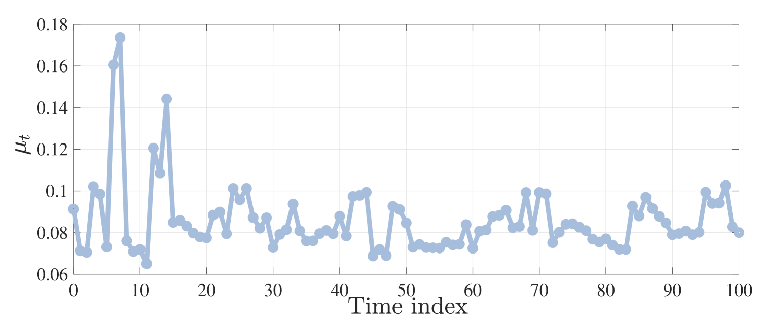
We apply the proposed methods to a system of 10 homogeneous charging stations over 100 time steps with fixed net energy ($c_{t}=10$). Namely, $\gamma_{i,t}=-1/100|t-50|+1$ and $\kappa_{i,t}=2$ for $i\in\{1,\ldots,10\}$. The charging cost distribution is informed by $\mu_{t}$ and $\sigma_{t}$; in our case, $\mu_{t}$ is the time series data of CAISO real-time prices deposited in Fig 1 (taken from http://www.energyonline.com) and $\sigma_{t}=1$. Given these parameter values, the cost is $\alpha_{t}$-strongly convex and $\beta_{t}$-jointly smooth with $\alpha_{t}=\beta_{t}=2$. Following the results in [27], the distributional maps are $\varepsilon_{t}$-sensitive with $\varepsilon_{t}=\mu_{t}$. The sequence of performatively stable points are computed in closed form by solving the KKT equations.

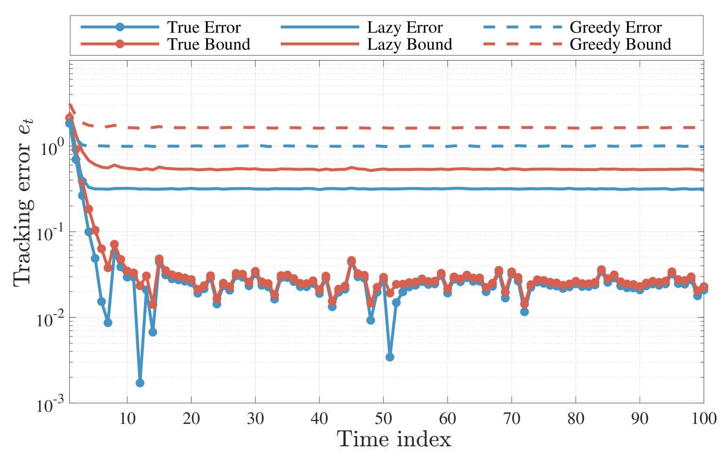
For each experiment, we run OPGD and OSPGD with fixed step size $\eta_{t}=0.3$ by drawing initial state $x_{0}$ uniformly from a sphere of radius $5$. For OSPGD, we compute the mean tracking error for both greedy and lazy deployments. The mean tracking error for each is computed via Monte Carlo simulation using $1,000$ realizations of the initial state.

In Fig. 2, we illustrate the tracking errors and corresponding upper bounds presented in Theorems 3.4 and 4.1. “True” (i.e., true gradient) refers to the OPGD, “greedy” to the OSPGD with $N_{t}=1$, and “lazy” to the OSPGD with $N_{t}=10$. We notice that the upper bound curve mimics the evolution of the tracking error; yet, in the instance of OSPGD the relationship is looser relative to the OPGD curves.

This paper considered online gradient and stochastic gradient methods for tracking solutions of time-varying stochastic optimization problems with decision-dependent distributions. Under a distributional sensitivity assumption, we derived explicit error bounds for the two methods. In particular, we derived convergence in expectation and in high probability for the OSPGD by assuming that the error in the gradient follows a sub-Weibull distribution. To the best of our knowledge, our convergence results for online gradient methods are the first in the literature for time-varying stochastic optimization problems with decision-dependent distributions.

References

- [1] C. Wilson, Y. Bu, and V. V. Veeravalli, “Adaptive sequential machine learning,” Sequential Analysis, vol. 38, no. 4, pp. 545–568, 2019.
- [2] J. L. Mathieu, D. S. Callaway, and S. Kiliccote, “Examining uncertainty in demand response baseline models and variability in automated responses to dynamic pricing,” in IEEE Conference on Decision and Control, 2011, pp. 4332–4339.
- [3] W. Tushar, W. Saad, H. V. Poor, and D. B. Smith, “Economics of electric vehicle charging: A game theoretic approach,” IEEE Transactions on Smart Grid, vol. 3, no. 4, pp. 1767–1778, 2012.
- [4] A. Hauswirth, S. Bolognani, G. Hug, and F. Dörfler, “Optimization algorithms as robust feedback controllers,” arXiv preprint arXiv:2103.11329, 2021.
- [5] G. Bianchin, M. Vaquero, J. Cortes, and E. Dall’Anese, “Online stochastic optimization for unknown linear systems: Data-driven synthesis and controller analysis,” arXiv preprint arXiv:2108.13040, 2021.
- [6] J. Perdomo, T. Zrnic, C. Mendler-Dünner, and M. Hardt, “Performative prediction,” in International Conference on Machine Learning. PMLR, 2020, pp. 7599–7609.
- [7] D. Drusvyatskiy and L. Xiao, “Stochastic optimization with decision-dependent distributions,” arXiv preprint arXiv:2011.11173, 2020.
- [8] A. Y. Popkov, “Gradient methods for nonstationary unconstrained optimization problems,” Automation and Remote Control, vol. 66, no. 6, pp. 883–891, 2005.
- [9] D. D. Selvaratnam, I. Shames, J. H. Manton, and M. Zamani, “Numerical optimisation of time-varying strongly convex functions subject to time-varying constraints,” in IEEE Conference on Decision and Control, 2018, pp. 849–854.
- [10] A. Mokhtari, S. Shahrampour, A. Jadbabaie, and A. Ribeiro, “Online optimization in dynamic environments: Improved regret rates for strongly convex problems,” in IEEE Conference on Decision and Control, 2016, pp. 7195–7201.
- [11] A. Simonetto, “Time-varying convex optimization via time-varying averaged operators,” arXiv preprint arXiv:1704.07338, 2017.
- [12] L. Madden, S. Becker, and E. Dall’Anese, “Bounds for the tracking error of first-order online optimization methods,” Journal of Optimization Theory and Applications, vol. 189, no. 2, pp. 437–457, 2021.
- [13] J. Cutler, D. Drusvyatskiy, and Z. Harchaoui, “Stochastic optimization under time drift: iterate averaging, step decay, and high probability guarantees,” arXiv preprint arXiv:2108.07356, 2021.
- [14] X. Cao, J. Zhang, and H. V. Poor, “Online stochastic optimization with time-varying distributions,” IEEE Tran. on Automatic Control, vol. 66, no. 4, pp. 1840–1847, 2021.
- [15] I. Shames and F. Farokhi, “Online stochastic convex optimization: Wasserstein distance variation,” arXiv preprint arXiv:2006.01397, 2020.
- [16] C. Wilson, V. V. Veeravalli, and A. Nedić, “Adaptive sequential stochastic optimization,” IEEE Tran. on Automatic Control, vol. 64, no. 2, pp. 496–509, 2018.
- [17] C. Mendler-Dünner, J. C. Perdomo, T. Zrnic, and M. Hardt, “Stochastic optimization for performative prediction,” arXiv preprint arXiv:2006.06887, 2020.
- [18] Z. Izzo, L. Ying, and J. Zou, “How to learn when data reacts to your model: performative gradient descent,” arXiv preprint arXiv:2102.07698, 2021.
- [19] M. Vladimirova, S. Girard, H. Nguyen, and J. Arbel, “Sub-Weibull distributions: Generalizing sub-Gaussian and sub-Exponential properties to heavier tailed distributions,” Stat, vol. 9, no. 1, p. e318, 2020.
- [20] R. Vershynin, High-dimensional probability: An introduction with applications in data science. Cambridge University press, 2018.
- [21] L. V. Kantorovich and S. Rubinshtein, “On a space of totally additive functions,” Vestnik of the St. Petersburg University: Mathematics, vol. 13, no. 7, pp. 52–59, 1958.
- [22] K. C. Wong, Z. Li, and A. Tewari, “Lasso guarantees for -mixing heavy-tailed time series,” The Annals of Statistics, vol. 48, no. 2, pp. 1124 – 1142, 2020.
- [23] N. Bastianello, L. Madden, R. Carli, and E. Dall’Anese, “A stochastic operator framework for inexact static and online optimization,” arXiv preprint arXiv:2105.09884, 2021.
- [24] Z.-P. Jiang and Y. Wang, “Input-to-state stability for discrete-time nonlinear systems,” Automatica, vol. 37, no. 6, pp. 857–869, 2001.
- [25] A. Nemirovski, A. Juditsky, G. Lan, and A. Shapiro, “Robust stochastic approximation approach to stochastic programming,” SIAM Journal on optimization, vol. 19, no. 4, pp. 1574–1609, 2009.
- [26] L. Hodgkinson and M. W. Mahoney, “Multiplicative noise and heavy tails in stochastic optimization,” arXiv preprint arXiv:2006.06293, 2020.
- [27] C. R. Givens and R. M. Shortt, “A class of Wasserstein metrics for probability distributions.” Michigan Mathematical Journal, vol. 31, no. 2, pp. 231 – 240, 1984.