Online Prototypes and Class-Wise Hypergradients for Online Continual Learning with Pre-Trained Models
Abstract
Continual Learning (CL) addresses the problem of learning from a data sequence where the distribution changes over time. Recently, efficient solutions leveraging Pre-Trained Models (PTM) have been widely explored in the offline CL (offCL) scenario, where the data corresponding to each incremental task is known beforehand and can be seen multiple times. However, such solutions often rely on 1) prior knowledge regarding task changes and 2) hyper-parameter search, particularly regarding the learning rate. Both assumptions remain unavailable in online CL (onCL) scenarios, where incoming data distribution is unknown and the model can observe each datum only once. Therefore, existing offCL strategies fall largely behind performance-wise in onCL, with some proving difficult or impossible to adapt to the online scenario. In this paper, we tackle both problems by leveraging Online Prototypes (OP) and Class-Wise Hypergradients (CWH). OP leverages stable output representations of PTM by updating its value on the fly to act as replay samples without requiring task boundaries or storing past data. CWH learns class-dependent gradient coefficients during training to improve over sub-optimal learning rates. We show through experiments that both introduced strategies allow for a consistent gain in accuracy when integrated with existing approaches. We will make the code fully available upon acceptance. ††Correspondance to Nicolas Michel, nicolas@cvm.t.u-tokyo.ac.jp
1 Introduction
Continual Learning (CL) has gained significant popularity in the past decade (Kirkpatrick et al., 2017; Rao et al., 2019; Zhou et al., 2024a). The main idea relies on learning from a sequence of data rather than a fixed dataset. Consequently, the data distribution can change, and new classes can appear, which often leads to the well-known problem of Catastrophic Forgetting (French, 1999). In this paper, we focus on the Class Incremental Learning problem (Hsu et al., 2018).
Fundamentally, Continual Learning scenarios can be divided into two categories: offline Continual Learning (offCL) (Tiwari et al., 2022) and online Continual Learning (onCL) (Mai et al., 2022). The former and most popular scenario assumes that this sequence of data is clearly defined in various tasks and that the learning process on a given task is completely analogous to traditional learning. Namely, data in each task are i.i.d. and the model can be trained for several epochs on a given task before visiting the next one. On the contrary, onCL assumes that the incoming data is analogous to a stream and therefore cannot be seen more than once by the model to enforce fast adaptation. Moreover, in the objective of moving toward more realistic scenarios, various studies now consider unclear or blurry task boundaries (Moon et al., 2023; Koh et al., 2023; Bang et al., 2022) which completely disables task information usage. Such differences make methods designed for offCL seldom transferable to onCL as the vast majority relies on leveraging multiple epochs, as well as task boundary information. Recent representation-based methods such as RANPAC (McDonnell et al., 2024) or EASE (Zhou et al., 2024b) are good examples, which require clear task boundaries to compute the task-specific representations, making them incompatible with onCL. While the difficulty of not having access to task information in onCL has been addressed in various studies (Aljundi et al., 2019; Koh et al., 2023; Moon et al., 2023; Michel et al., 2024), it remains under-explored when considering Pre-Trained Models (PTM).
Another significant problem when considering the online continuous adaption of a model is the inability to estimate the optimal hyper-parameters. As the dataset of interest cannot be stored, typical hyper-parameters such as the Learning Rate (LR) should not be optimized to fully reflect the problem at hand. However, such consideration has been widely omitted in current onCL literature where LR selection strategies are often unclear. A common practice is to choose the same fixed Learning Rate (LR) and optimizer for all considered methods (Gu et al., 2022; Mai et al., 2021; Moon et al., 2023; Lin et al., 2023), typically Stochastic Gradient Descent (SGD) with LR value of . This design choice is extremely limited as various methods and datasets have different optimal LR. It is also well-known that a suboptimal LR has a critical impact on the final performances. Another strategy is to estimate the best hyper-parameters on a given dataset and to transfer them onto other configurations (Michel et al., 2024). While more realistic, there is no guarantee that such hyper-parameters can realistically be transferred from one dataset to another.
In this paper, we propose to improve the usage of PTM in onCL by addressing both previously introduced problems. Firstly, we solve the lack of task boundaries by simply computing Online Prototypes (OP) to recalibrate the model’s final layer towards previous classes similar to the replay strategy at the representation level. Secondly, we adapt Hypergradients (Baydin et al., 2018) to onCL by considering class-wise gradients (He, 2024); which we call Class-Wise Hypergradients (CWH). In summary, our contributions are as follows:
-
•
we introduce the problem of LR selection in onCL, which to the best of our knowledge remained largely unexplored;
-
•
we tackle onCL difficulties by leveraging Online Prototypes and introducing Class-Wise Hypergradients;
-
•
we demonstrate superior performances when combining such elements with state-of-the-art offCL methods, leveraging PTM in OCL across several datasets and initial LR.
2 Related Work
2.1 PTM based Continual Learning
In recent years, pre-trained models (PTMs) have been widely utilized in offCL (McDonnell et al., 2024; Lin et al., 2023; Zhou et al., 2024b; Smith et al., 2023; Wang et al., 2022b). However, their application in onCL remains largely unexplored, partly because most existing methods heavily depend on task boundaries, i.e., explicit knowledge of when the task changes. This is often assumed in pair with clear boundaries, meaning that all classes from the previous task are suddenly unavailable while all new classes encountered belong to the new task. With real-world streaming data, such a situation is equally unlikely.
2.2 Online Continual Learning
In onCL, incoming data can be seen only once, analogous to a continuous data stream (He et al., 2020). Therefore, clear boundaries are unlikely to be available and several studies suggest working in boundary-free scenarios (Buzzega et al., 2020) where task change is unknown. However, if the change is clear, it can easily be inferred. In that sense, blurry boundary setting have been proposed (Moon et al., 2023; Koh et al., 2023; Bang et al., 2022; Michel et al., 2024) in previous work. In particular, we are interested in the Si-Blurry setting (Moon et al., 2023) where not only task change is blurry, but some classes can appear or disappear during multiple tasks, which brings the experimental setup one step closer to real-world scenarios while being more challenging. While numerous studies rely on prototypes for Continual Learning (McDonnell et al., 2024; Lin et al., 2023; Zhou et al., 2024b), such representation-based methods must generally be combined with task boundary knowledge as prototypes are updated at the end of each task. In onCL, prototypes are harder to capitalize on when training a model from scratch due to the shift of representations hindering prototype computation (Caccia et al., 2022). However, when working with PTM, such a shift is drastically reduced as representations are already of high quality, making the usage of prototypes more efficient.
2.3 Hypergradients and Gradient Re-Weighting
Hypergradient (Baydin et al., 2018; Almeida et al., 1999) addresses the problem of finding the optimal learning rate in conventional training scenarios. In that sense, the authors proposed to derive a gradient descent algorithm to learn the LR. Notably, they demonstrate that computing the dot product between gradients from previous steps is sufficient to complete one step of the learning rate update rule, with the index of the current step, the parameters, and the loss function. However, such techniques have been, to the best of our knowledge, developed solely for offline scenarios at a global level. In Continual Learning, gradient re-weighting strategies have been designed for replay-based CL methods. Notably, previous work proposed to re-weight the gradient at the loss level to mitigate its accumulation during training in CL context, also called gradient imbalance (Guo et al., 2023). Recently, to compensate for the class imbalance, class-wise manually defined weights in the last Fully Connected (FC) layer have been leveraged (He, 2024). Our work on Class-Wise Hypergradients lies at the cross-road between Hypergradients and Gradient Re-Weighting.
3 Learning Rate Selection in Online Continual Learning
3.1 Preliminary
Generally, the problem of CL is defined as training a model parameterized by on a sequence of tasks where each task of index is defined by its corresponding dataset , each potentially being drawn from a different distribution. In the case Class Incremental Learning (Hsu et al., 2018), we have , the data-label pairs. In offCL, the model is trained sequentially on each task while other task data is unavailable. For onCL, while the model is similarly trained sequentially on each task, only the data of the current batch is available and can be seen only once during training. The final objective in offCL and onCL is the same: to maximize performance across all tasks. Equivalently, to minimize the average loss across all tasks:
| (1) |
3.2 Finding the Optimal Learning Rate
Traditional Learning.
Finding the optimal LR is a common challenge inherent to training any deep neural network with gradient-descent-based optimization techniques. Mainstream methods heavily rely on LR schedulers (He et al., 2016; Vaswani, 2017), which would typically decrease the LR value over time after each epoch. Of course, the starting value as well as the speed of the learning rate decrease must still be found. To this end, grid search remains a popular and powerful technique in traditional learning scenarios.
LR in offCL.
Similarly, in offCL, state-of-the-art methods have adopted LR schedulers (Smith et al., 2023; Wang et al., 2022b; Roy et al., 2024), however their strategy regarding finding hyperparameters is often unclear. While grid search is feasible in offCL at the task level, clear limitations can be identified. Firstly, finding the best initial LR at a given task on dataset does not give any guarantee regarding the LR to use on subsequent datasets . Secondly, a suboptimal learning rate with regard to can lead to overall higher performances when evaluating on . Indeed, as discussed in the work of Mirzadeh et al. (Mirzadeh et al., 2020), large learning rates can disturb weights that are important for previous tasks. The loss minimized at specific timestep conflicts with the overall objective since the distribution of incoming data from and differ.
LR in onCL.
Determining the optimal learning rate in onCL is even more challenging. In addition to the offCL challenges mentioned earlier, even grid search at the task level is unavailable. The online scenario constrains the model to see the incoming data only once, usually in small batches, making any hyper-parameter search completely impossible. A long-lasting strategy to train in this context is to use the same pre-determined fixed LR and optimizer for all considered methods (Gu et al., 2022; Mai et al., 2021; Moon et al., 2023; Lin et al., 2023), typically Stochastic Gradient Descent (SGD) with an LR value of . While the choice of SGD has been found to lead to better generalization in some cases (Keskar & Socher, 2017), the reasoning behind this choice remains unclear in the literature and presents significant limitations. Firstly, there is no justification for different methods, with different losses, to benefit equally from using the same learning and optimizer. Secondly, as discussed in Section 5.3, it is apparent that some methods are more sensitive to LR change than others. To overcome this, some studies look for the best hyper-parameters offline for all considered methods before transferring such parameters to other setups (Michel et al., 2024). However, this remains insufficient as the optimal learning rate most likely varies from one dataset to the other. Despite the well-known critical impact of a suboptimal LR on final performance, the problem of selecting the best LR remains largely overlooked by the Online Continual Learning community.
3.3 LR and Learning Behavior in onCL
Impact on Stability-Plasticity.
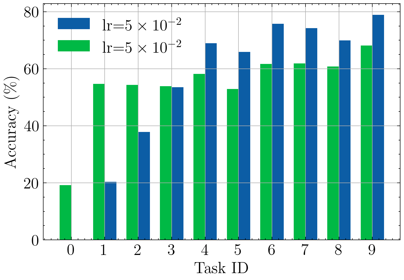
It is clear that selecting an appropriate learning rate is essential for optimal performance. In standard scenarios, the impact of its choice on loss minimization and convergence speed has been extensively studied (Ruder, 2016). For offCL, previous studies have considered to impact of the LR on forgetting (Mirzadeh et al., 2020). Notably, a higher LR would increase forgetting, and vice-versa. Intuitively, the learning rate gives a direct control on the plasticity-stability tradeoff (Wang et al., 2024). To confirm such behavior in onCL, we experiment with larger and smaller LR values. As it can be seen in Figure 1, when trained with a higher learning rate (), the model tends to obtain higher performances on the latest tasks while exhibiting especially low performances on earlier tasks. When trained with a lower LR (), the model tends to achieve better performance on earlier tasks compared to training with a higher LR. In other words, a high LR value induces more plasticity and less stability, and vice-versa.
FC Layer Behavior.
For PTM in offCL, previous work considers different LR values for different layers (McDonnell et al., 2024). Notably, leveraging a higher LR in the last FC layer seems beneficial to the training procedure. In onCL, we observe similar behavior. To do so, we experiment with CODA (Smith et al., 2023) where we multiply the gradient values with regard to the final layer by a coefficient , with falling back to the regular CODA training in onCL. Such results are presented in Table 1 on various onCL datasets. It can be seen that increasing the LR of the final FC layer can often lead to an improvement in terms of average performances, even though in cases of lower LR such an effect is barely noticeable. While this naive approach can lead to improvements in certain scenarios, it induces more hyper-parameter tuning and considers the same LR strategy for each class.
| Learning Rate | |||
|---|---|---|---|
| CIFAR100 | |||
| CODA ( | 73.36±1.88 | 81.69±1.48 | 64.98±3.47 |
| CODA () | 73.40±1.88 | 81.74±2.16 | 66.90±0.47 |
| CODA () | 73.41±1.84 | 81.43±1.94 | 64.10±3.41 |
| CODA () | 73.41±1.88 | 81.75±0.87 | 67.93±1.63 |
| ImageNet-R | |||
| CODA ( | 24.62±1.67 | 64.03±1.81 | 33.18±3.59 |
| CODA () | 24.62±1.66 | 64.93±0.85 | 31.89±4.07 |
| CODA () | 24.62±1.66 | 65.25±0.21 | 36.85±8.25 |
| CODA () | 24.62±1.66 | 64.87±0.62 | 35.32±5.44 |
| CUB | |||
| CODA ( | 22.06±0.87 | 65.28±3.07 | 40.25±12.5 |
| CODA () | 22.03±0.9 | 65.70±2.48 | 51.15±0.94 |
| CODA () | 22.03±0.9 | 65.06±2.07 | 48.26±1.7 |
| CODA () | 22.05±0.89 | 65.70±2.81 | 45.32±6.52 |
4 Proposed Method
4.1 Motivations
As discussed in Section 3, LR is critical in onCL as it not only has a direct impact on the plasticity-stability trade-off, it is near impossible to use the optimal value. While previous studies highlight the need for different LR at the layer level, the case of different learning rates at the class level is still in its infancy. Following the analysis described in Section 3.3, we make the hypothesis that a class-wise LR strategy focusing on the last FC layer is crucial for onCL. The intuition is that different classes require different learning rates so that the model can adapt its stability-plasticity tradeoff not only over time, but also over classes. In that sense, we reckon hypergradients (Baydin et al., 2018) to be adequate for improving over non-optimal initial LR values. However, hypergradients are not designed for the onCL scenario and a naive implementation leads to a severe performance drop. Indeed, hypergradient computation is identical regardless of the network layer or the classes. Inspired by the work of He et al. (He, 2024), we propose learning how to rescale the gradient coefficient of the last FC layer, class-wise, using hypergradient learning theory.
Additionally, to adapt PTM-based methods to the onCL scenario further, we leverage the stability of the output representation of PTM by computing Online Prototypes.
4.2 Class-Wise Hypergradients
Let us consider a model parameterized by such that for an input , with the dimension of the input space, we have , with , the number of classes, the dimension of the output of and . In this context, would typically be a PTM and the weight of the final FC layer (including the bias). Looking at the final FC layer , for a learning rate , we can write the gradient-based weight update:
| (2) |
with the iteration index. Here, we omit the input data for simplicity. Then, for any class index , we can write the update rule of the weights corresponding to :
| (3) |
with the column of . Building upon previous studies (He, 2024), we introduce step-dependent class-wise weighting coefficients, leading to the following update rule:
| (4) |
with , class dependent gradient weighting coefficient at index . While those coefficients were traditionally introduced to compensate for class interference, and computed with hand-crafted rules, we propose to learn them through an online adaptive rule based on hypergradients theory. In particular, we want to construct a higher level update for such that, in the case:
| (5) |
with the hypergradient learning rate. To compute the partial derivative we apply the chain rule and make use of the fact that , such that:
| (6) | ||||
| (7) |
The resulting Class-Wise Hypergradient update becomes:
| (8) |
With . Naturally, this introduces an undesired extra-hyperparameter. We discuss this limitation in Section 6. For clarity, the relation presented in Eq. (8) relies on an SGD update. In practice, we favor a momentum-based update, notably Adam (Kingma & Ba, 2014). We follow the guidelines of Baydin et al. (Baydin et al., 2018) regarding its implementation and give more detail in Appendix A.
4.3 Online Prototypes
In order to reduce forgetting in the last layer, we compute Online Prototypes (OP) of each class during training. For a given class , the class prototype computed over samples is updated when encountering a new sample . For simplicity, we omit the index in going forward. Therefore, the prototype update rule is:
| (9) |
with the encountered sample of class . For all classes, prototypes are initialized such that . Prototypes are then used to recalibrate the final FC layer, analogous to replaying the average of past data representation during training. In that sense, we define the prototype-based loss term as:
| (10) |
with . is the cross-entropy with regard to prototypes of encountered classes. OP acts as simple and low-budget memory data.
4.4 Overall Training Procedure
The approach relies on two components that are orthogonal to most existing methods, as long as the model optimizes a final FC layer for classification. In that sense, we propose to integrate it into various state-of-the-art baselines relying on PTM, notably prompt-based approaches. To do so, if we consider to be the loss of the baseline method, to which we attach both components OP and CWH, we have the overall loss to minimize:
| (11) |
A Pytorch-like (Paszke et al., 2019) pseudo code is given in Algorithm 1. Additionally, we leverage batch-wise masking to consider the logits of classes that are only present in the current batch. More details can be found in the Appendix A. Similarly, note that the bias has been omitted for simplicity.
5 Experiments
In the following sections experiment with combining our proposed approach with several flagship CL approaches.
| Dataset | CIFAR100 | Imagenet-R | CUB | |||||||||
|---|---|---|---|---|---|---|---|---|---|---|---|---|
| Learning Rate | Avg. | Avg. | Avg. | |||||||||
| L2P | 67.86±2.12 | 78.18±1.29 | 68.54±0.98 | 71.53±1.46 | 25.93±3.87 | 55.56±1.81 | 50.18±1.36 | 43.89±2.35 | 20.15±2.69 | 55.21±2.22 | 51.27±2.09 | 42.21±2.33 |
| + OP | 80.74±1.08 | 85.73±0.06 | 79.11±0.87 | 81.86±0.67 | 47.96±1.2 | 68.68±1.13 | 60.57±0.96 | 59.07±1.1 | 48.20±0.84 | 83.51±1.49 | 73.29±1.2 | 68.33±1.18 |
| + CWH | 81.73±0.93 | 85.52±0.1 | 78.16±1.43 | 81.80±0.82 | 53.18±1.68 | 68.89±1.11 | 58.38±2.01 | 60.15±1.6 | 58.84±0.9 | 83.98±1.3 | 72.78±2.1 | 71.87±1.43 |
| DualPrompt | 62.21±1.21 | 77.36±0.46 | 65.10±0.92 | 68.22±0.86 | 25.34±1.32 | 59.11±0.54 | 53.15±3.01 | 45.87±1.62 | 21.77±3.13 | 65.34±1.22 | 53.59±2.17 | 46.90±2.17 |
| + OP | 78.16±1.31 | 85.35±0.76 | 68.28±1.95 | 77.26±1.34 | 49.10±1.36 | 67.68±0.37 | 57.40±2.1 | 58.06±1.28 | 55.06±1.34 | 86.13±0.84 | 69.72±1.69 | 70.30±1.29 |
| + CWH | 79.78±1.29 | 85.08±0.68 | 67.27±1.77 | 77.38±1.25 | 54.59±1.07 | 67.55±0.51 | 55.03±4.77 | 59.06±2.12 | 66.71±0.95 | 86.67±0.91 | 69.10±3.73 | 74.16±1.86 |
| CODA | 73.36±1.88 | 81.69±1.48 | 64.98±3.47 | 73.34±2.28 | 24.62±1.67 | 64.03±1.81 | 33.18±3.59 | 40.61±2.36 | 22.06±0.87 | 65.28±3.07 | 40.25±12.5 | 42.53±5.48 |
| + OP | 85.74±0.7 | 86.16±0.64 | 72.42±0.8 | 81.44±0.71 | 49.39±0.87 | 72.30±1.7 | 38.72±3.57 | 53.47±2.05 | 55.35±1.66 | 81.21±2.33 | 59.59±8.63 | 65.38±4.21 |
| + CWH | 86.92±0.66 | 85.45±1.37 | 70.11±0.49 | 80.83±0.84 | 55.63±0.97 | 70.12±2.17 | 41.32±5.62 | 55.69±2.92 | 66.74±1.79 | 81.78±2.28 | 60.26±3.09 | 69.59±2.39 |
| ConvPrompt | 78.61±1.25 | 85.76±0.43 | 74.40±0.69 | 79.59±0.79 | 30.98±0.97 | 66.66±1.33 | 17.45±27.19 | 38.36±9.83 | 31.16±1.04 | 70.78±2.65 | 34.13±16.8 | 45.36±6.83 |
| + OP | 88.70±0.77 | 90.41±0.54 | 78.59±6.67 | 85.90±2.66 | 53.82±1.41 | 74.79±1.13 | 21.60±26.5 | 50.07±9.68 | 57.42±3.4 | 86.66±1.35 | 42.19±29.36 | 62.09±11.37 |
| + CWH | 88.86±0.63 | 90.16±0.21 | 80.94±5.31 | 86.65±2.05 | 53.17±1.0 | 72.94±1.31 | 34.90±28.87 | 53.67±10.39 | 65.02±3.77 | 84.56±0.75 | 65.42±19.02 | 71.67±7.85 |
| MVP | 49.64±0.92 | 57.63±2.13 | 43.40±1.02 | 50.22±1.36 | 28.75±0.42 | 38.25±0.54 | 28.87±0.79 | 31.96±0.58 | 28.39±0.81 | 44.10±1.63 | 29.96±0.81 | 34.15±1.08 |
| + OP | 82.63±0.91 | 85.61±0.12 | 56.16±1.3 | 74.80±0.78 | 58.04±1.05 | 62.08±0.29 | 47.50±1.9 | 55.87±1.08 | 72.06±2.05 | 85.86±1.63 | 59.64±4.41 | 72.52±2.7 |
| + CWH | 83.64±0.59 | 85.44±0.11 | 61.60±1.27 | 76.89±0.66 | 60.39±0.74 | 62.25±0.35 | 50.09±3.7 | 57.58±1.6 | 77.15±2.0 | 85.21±1.44 | 70.49±3.35 | 77.62±2.26 |
| Dataset | CIFAR100 | Imagenet-R | CUB | |||||||||
|---|---|---|---|---|---|---|---|---|---|---|---|---|
| Learning Rate | Avg. | Avg. | Avg. | |||||||||
| L2P | 47.37±6.28 | 71.45±6.51 | 67.35±4.82 | 62.06±5.87 | 13.71±2.27 | 44.02±4.47 | 44.1±0.84 | 33.94±2.53 | 7.51±2.91 | 46.57±1.18 | 47.25±2.27 | 33.78±2.12 |
| + OP | 69.68±5.59 | 82.05±4.96 | 79.25±2.35 | 76.99±4.3 | 32.99±2.23 | 61.34±1.93 | 55.6±2.49 | 49.98±2.22 | 24.46±6.64 | 76.53±1.7 | 69.52±2.46 | 56.84±3.6 |
| + CWH | 73.01±5.23 | 82.39±3.66 | 78.17±2.35 | 77.86±3.75 | 39.22±2.03 | 60.99±1.84 | 54.41±1.8 | 51.54±1.89 | 36.45±6.31 | 77.0±1.97 | 67.7±2.13 | 60.38±3.47 |
| DualPrompt | 46.07±3.25 | 72.03±5.63 | 65.72±5.12 | 61.27±4.67 | 15.29±0.68 | 50.13±1.32 | 45.84±2.81 | 37.09±1.6 | 12.46±1.5 | 57.03±0.4 | 51.47±1.25 | 40.32±1.05 |
| + OP | 66.35±9.42 | 82.15±2.72 | 72.3±2.01 | 73.6±4.72 | 36.79±1.05 | 59.78±0.95 | 51.74±2.81 | 49.44±1.6 | 37.91±2.38 | 79.64±1.99 | 67.89±1.59 | 61.81±1.99 |
| + CWH | 72.41±3.65 | 82.06±2.32 | 71.91±1.42 | 75.46±2.46 | 42.46±0.91 | 59.49±0.81 | 50.56±2.17 | 50.84±1.3 | 50.26±2.25 | 80.48±1.83 | 66.59±2.07 | 65.78±2.05 |
| CODA | 54.38±3.63 | 77.23±7.11 | 64.04±5.82 | 65.22±5.52 | 15.89±2.47 | 56.38±0.51 | 28.47±2.74 | 33.58±1.91 | 12.52±1.65 | 57.6±1.34 | 45.79±1.86 | 38.64±1.62 |
| + OP | 75.02±2.02 | 84.0±4.3 | 73.12±1.29 | 77.38±2.54 | 37.85±1.92 | 64.55±0.39 | 31.84±14.84 | 44.75±5.72 | 36.83±1.88 | 76.25±0.29 | 60.6±4.42 | 57.89±2.2 |
| + CWH | 77.71±2.94 | 84.39±3.56 | 74.61±1.69 | 78.9±2.73 | 43.45±1.6 | 63.53±1.72 | 34.93±1.11 | 47.3±1.48 | 49.24±1.16 | 77.53±1.32 | 56.81±2.2 | 61.19±1.56 |
| ConvPrompt | 42.76±1.76 | 48.18±1.43 | 26.54±22.0 | 39.16±8.4 | 15.02±0.43 | 33.17±1.82 | 6.2±9.66 | 18.13±3.97 | 13.93±1.78 | 32.0±0.71 | 21.33±6.09 | 22.42±2.86 |
| + OP | 49.96±2.01 | 51.65±2.39 | 47.29±2.43 | 49.63±2.28 | 28.79±2.4 | 38.75±1.62 | 17.32±14.38 | 28.29±6.13 | 30.49±2.79 | 43.42±2.45 | 11.18±10.9 | 28.36±5.38 |
| + CWH | 49.72±2.03 | 51.95±2.13 | 47.47±2.32 | 49.71±2.16 | 28.0±2.7 | 38.35±2.09 | 16.92±13.97 | 27.76±6.25 | 33.79±3.34 | 42.3±1.46 | 36.74±3.2 | 37.61±2.67 |
| MVP | 44.32±2.27 | 60.96±5.42 | 52.29±4.65 | 52.52±4.11 | 23.65±0.56 | 35.5±0.16 | 32.54±0.91 | 30.56±0.54 | 23.87±2.24 | 42.85±0.37 | 34.64±1.72 | 33.79±1.44 |
| + OP | 77.16±4.91 | 82.52±2.78 | 62.56±2.99 | 74.08±3.56 | 51.21±0.65 | 56.94±1.07 | 46.49±2.16 | 51.55±1.29 | 65.55±2.24 | 80.93±0.97 | 61.42±0.21 | 69.3±1.14 |
| + CWH | 78.49±4.89 | 82.46±2.58 | 64.12±1.73 | 75.02±3.07 | 53.75±0.76 | 57.02±1.03 | 45.5±2.21 | 52.09±1.33 | 71.81±1.48 | 81.46±1.16 | 63.27±0.6 | 72.18±1.08 |
5.1 Metrics
Average Performances (AP).
We follow previous work and define the Average Performance (AP) as the average of the accuracies computed after each task during training (Zhou et al., 2024a). Formally, when training on , we define , the Average Accuracy (AA) as:
| (12) |
with the accuracy on task after training on . Building on this, we define the Average Performance (AP) as:
| (13) |
Performance Across LR.
To show the improvement in the case of unknown optimal LR, we propose to experiment with various LR values and report individual and averaged performances across these values. Specifically, we experiment for LR values in . The main motivation is that we reckon that the optimal LR is likely to fall into that range, therefore we wanna take into account the effect of experimenting with a learning rate that is either above or below the optimal value. Such a metric should emphasize the validity of the approach when the optimal LR is unknown and result in a fairer comparison than using the same LR blindly for every approach.
5.2 Experimental Setting
Baselines and Datasets.
In order to demonstrate the efficiency of our approach as presented in Algorithm 1, we integrate it with several state-of-the-art methods in offCL. Notably, L2P (Wang et al., 2022b), DualPrompt (Wang et al., 2022a), CODA (Smith et al., 2023), ConvPrompt (Roy et al., 2024). These methods are not naturally suited for the online case, so they had to be adapted. More details on the adaptation of such methods are in Appendix D. Additionally, we include one state-of-the-art onCL method that leverages PTM, MVP (Moon et al., 2023). We evaluate our method on CUB (Wah et al., 2011), ImageNet-R (Hendrycks et al., 2021) and CIFAR100 (Krizhevsky, 2012). More details in Appendix B.2.
Clear Boundaries.
We experiment in clear boundaries settings, for continuity with previous work, despite its lack of realism for onCL. In that sense, we consider an initial count of classes for the first task, with an increment of classes per task. This results in tasks with classes per task for CIFAR100, as well as tasks with classes per task for CUB and ImageNet-R.
Blurry Boundaries.
To evaluate our method in more realistic scenarios, we reckon the Si-Blurry (Moon et al., 2023) setting to be the most relevant to our study case. Specifically, we use their implementation of Stochastic incremental Blurry boundaries (Si-Blurry). We use the same number of tasks as for the clear setting. In this case, some classes can appear or disappear during training and the transitions are not necessarily clear. More details on this setting can be found in Appendix E. To adequately adapt the proposed methods to the online problem, we use batch-wise masking. Specifically, we consider only the logits of the class that are observed in the current batch, for every method.
Implementation Details.
Every method is evaluated in the onCL context. Namely, only one pass over the data is allowed. The batch size is fixed at to simulate small data increments with a low storage budget in the context of fast adaptation. The PTM used is a ViT-base, pre-trained on ImageNet 21k. Every experiment was conducted over 3 runs and the average and standard deviation are displayed. Each run was conducted with a different seed, which equally impacted the task generation process. For all experiments, we use . More details on selection can be found in Section 6.2
5.3 Experimental Results
We combined our method with four offline approaches and one online state-of-the-art approach, all using PTM. As mentioned in Section 4.4, our method must be applied on the classification head, therefore prompt-based approaches are especially suited as they all leverage a final FC layer on top of the PTM representation for classification.
Average Performances.
We experiment in both clear and blurry settings and present the results in terms of Average Performance in Table 2 and Table 3. On top of datasets and boundary scenarios, we propose a novel evaluation procedure specific to the problem at hand. Namely, we present results for LR values in , as well as the AP across all these values. The objective is to observe how would the method perform on average when the optimal learning rate is unknown and might be far from optimal, by being either too high or too low. Therefore, in all cases, combining both proposed components leads to a significant improvement in AP over the baselines when looking at the average across learning rates, with up to improvement on CUB. Such improvements are observed in both blurry and clear scenarios, confirming the ability of our approach to perform in realistic and traditional contexts. Individual contributions of OP and CWH are detailed below.
Blurry Boundaries.
Even though performance improvement can be observed as well in the blurry scenario, all methods suffer from a significant drop when transitioning from one scenario to the other. Such behavior highlights the importance of focusing on more realistic setups in future research. In that sense, our method remains completely applicable regardless of the presence of boundaries.
Ablation Study.
To make apparent the contribution of each component of our method, we included the performances of the original baselines, followed by the performance of such baselines combined with OP (+ OP) and eventually the performance of the same baseline combined with prototypes and CWH (+ CWH). Such results are included in Tables 2 and 3. While it is clear that the usage of prototypes is largely beneficial, in some situations the addition of CWH can lead to a slight drop in performances. However, in those rare scenarios, the performance drop remains minimal with the maximum drop value being in the case of CODA on CUB with an LR of . In other cases, performance loss is around . Despite this limitation, it is important to note that the gain of including CWH is especially important for longer task sequences such as CUB, which is a more realistic scenario. Moreover, when the initial LR value is particularly low (), the gain of including CWH is generally more important. When fine-tuning PTM, it is common to start with low LR values. This property further confirms the ability of our approach to perform in realistic contexts.
| Initial LR | w/o OP | w/ OP | |
|---|---|---|---|
| Not Frozen | 8.97 | 8.18 | |
| 50.64 | 51.14 | ||
| Frozen | 77.10 | 85.73 | |
| 67.86 | 80.74 | ||
6 Discussions
6.1 Stability of OP
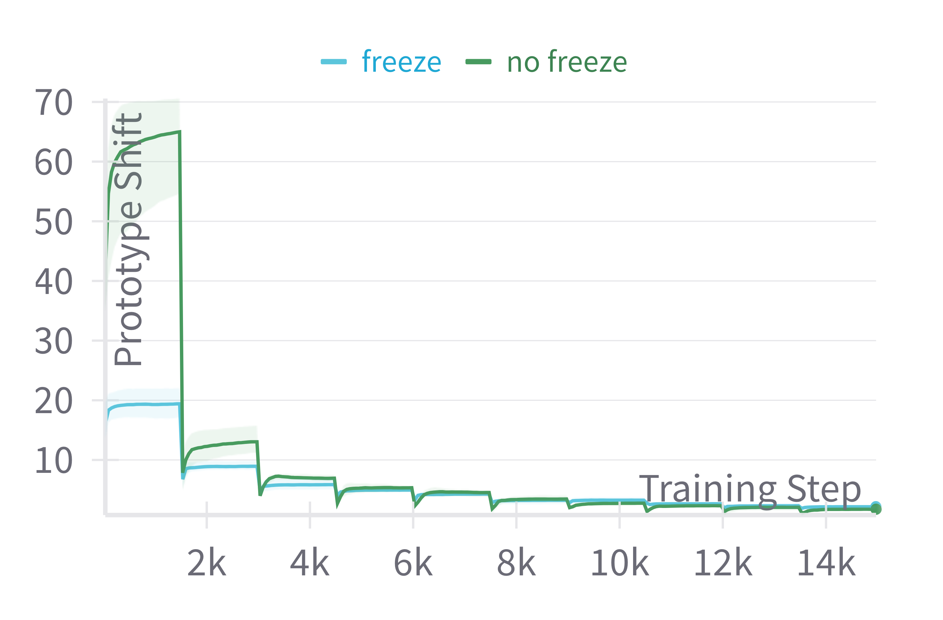
Despite its apparent simplicity, OP gives the largest performance gain. This is partially due to the fact that only the FC layer and the input prompts are trained, so the output prototypes are stable over time. In Table 4 we show that unfreezing intermediate weight not only drastically decreases overall performances but similarly negates the effect of OP significantly. Additionally, in Figure 2, we show the average Euclidean distance of Online Prototypes between two training step iterations. As we can see, the learned prototypes tend to stabilize rapidly over time, even more so when the intermediate weights remain frozen. This stability of the prototype indicates that even when computed online, they can be used as a reasonable proxy for class average representation.
6.2 Selecting
The main drawback of leveraging CWH is the addition of an extra hyper-parameter , whereas our objective is to reduce the dependency on hyper-parameters for onCL. However, we argue that selecting remains particularly simple. To demonstrate this, we experiment with , for an initial LR . In that case, is equivalent to disabling CWH. Such results are presented in Table 5. When the initial LR is lower, including CWH leads to an improvement in performance, especially when is large. Experimentally, this can be seen as a consequence of values increasing during training in all cases, as discussed in Section 6.3. Therefore, it is natural that lower initial LR values would benefit more from such a strategy. When the initial LR is large, as discussed in Section 5.3, a marginal drop in performance can be observed in some cases. However, the final performances remain stable for all values of , minimizing the need for hyperparameter search. Additionally, the lower the value of , the closer it is to the original method.
In conclusion, for higher LR we recommend lower values of , as their effect on the training is reduced. For lower LR, any value of leads to an improvement, however, higher values are recommended for optimal accuracy gain. Default values such as should lead to an increase in performances in most cases or a slight decrease in worst cases. Overall, selecting remains a simpler and more realistic task than doing a grid search in onCL.
| 0 | ||||||
|---|---|---|---|---|---|---|
| CIFAR100 | CODA | 75.02±2.02 | 76.04±2.29 | 77.71±2.94 | 77.75±2.99 | |
| DualPrompt | 66.35±9.42 | 70.57±3.7 | 72.41±3.65 | 72.45±3.65 | ||
| L2P | 69.68±5.59 | 71.11±5.56 | 73.01±5.23 | 73.10±5.19 | ||
| CODA | 73.12±1.29 | 72.88±1.72 | 74.61±1.69 | 75.77±2.91 | ||
| DualPrompt | 72.30±2.01 | 71.79±2.68 | 71.91±1.42 | 73.42±1.08 | ||
| L2P | 79.25±2.35 | 78.85±2.09 | 78.17±2.35 | 78.31±1.13 | ||
| ImageNet-R | CODA | 37.85±1.92 | 40.09±1.8 | 43.45±1.6 | 43.51±1.58 | |
| DualPrompt | 36.79±1.05 | 39.06±1.07 | 42.46±0.91 | 42.54±0.89 | ||
| L2P | 32.99±2.23 | 35.65±2.15 | 39.22±2.03 | 39.30±2.0 | ||
| CODA | 31.84±14.84 | 38.46±1.9 | 34.93±1.11 | 33.47±2.7 | ||
| DualPrompt | 51.74±2.81 | 50.86±2.3 | 50.56±2.17 | 50.05±2.2 | ||
| L2P | 55.60±2.49 | 55.25±1.55 | 54.41±1.8 | 54.80±1.12 | ||
| CUB | CODA | 36.83±1.88 | 40.28±1.95 | 49.24±1.16 | 49.40±1.07 | |
| DualPrompt | 37.91±2.38 | 41.26±2.59 | 50.26±2.25 | 50.46±2.16 | ||
| L2P | 24.46±6.64 | 27.88±6.59 | 36.45±6.31 | 36.63±6.38 | ||
| CODA | 60.60±4.42 | 56.58±4.14 | 56.81±2.2 | 58.42±6.1 | ||
| DualPrompt | 67.89±1.59 | 66.8±1.92 | 66.59±2.07 | 67.47±2.35 | ||
| L2P | 69.52±2.46 | 68.86±2.25 | 67.70±2.13 | 67.55±2.75 | ||
6.3 Values of learned
Trend and Distribution Across Classes.
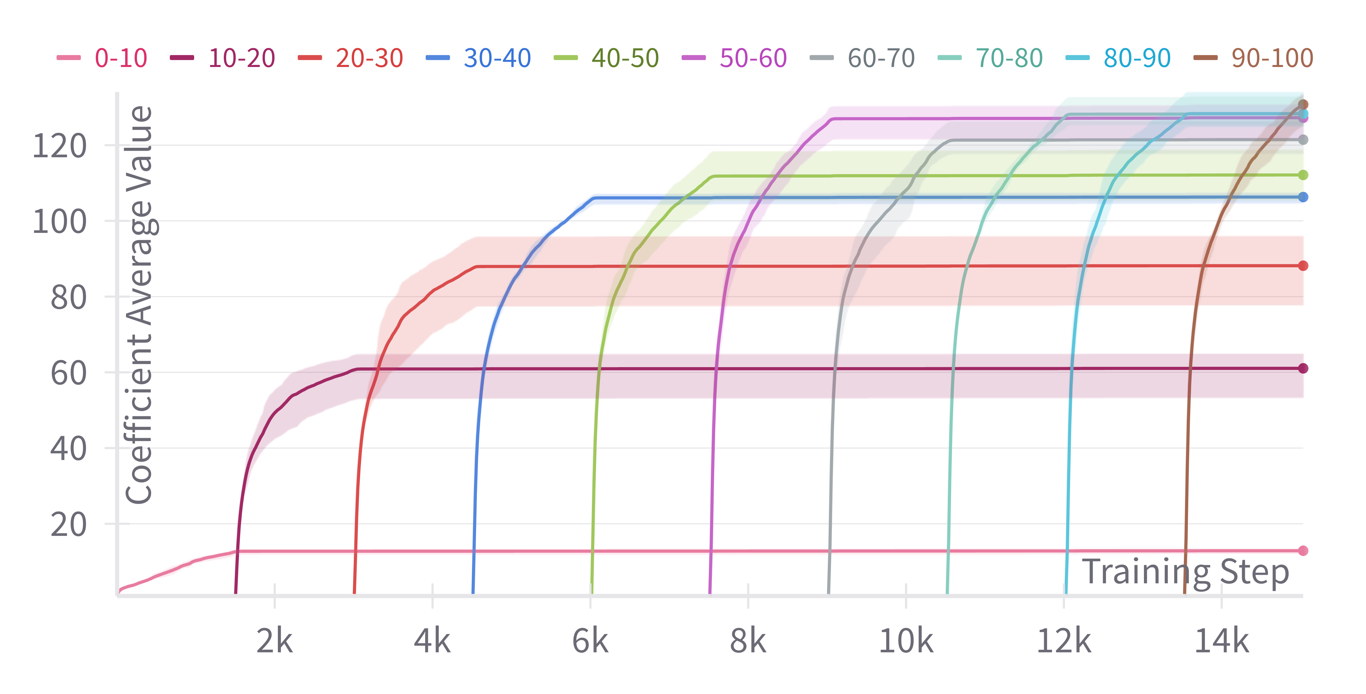
The class-wise coefficients are learned in each training step as described in Eq. (8). We report coefficients’ evolution in Figure 3. Firstly, learned coefficient values are superior to and increase during training. Such a trend is aligned with findings from previous studies suggesting adopting a higher LR value for the final FC layer (McDonnell et al., 2024). Secondly, it can be seen that coefficient values tend to be larger for later tasks than for earlier tasks. Intuitively, following the analysis from Section 3, this corresponds to giving more plasticity to newly encountered classes than older classes.
Relation with Learning Rate.
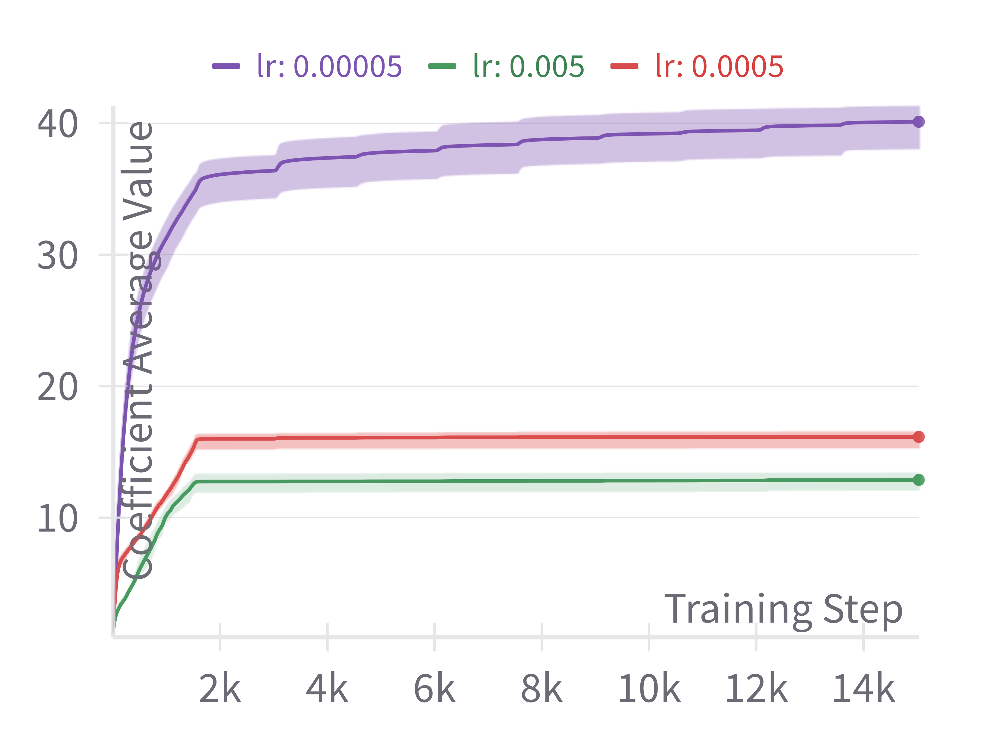
We investigate the behavior of the learned coefficient with regard to the initial LR. As we can see in Figure 4, the smaller the initial LR, the larger the values of learned coefficients. Intuitively, a smaller initial LR requires a larger compensation in the FC layer to reach a similar learning regime.
7 Conclusion
In this paper, we studied the problem of leveraging Pre-Trained Models in the context of Online Continual Learning. In that sense, we focused on two central problems. Namely, the unavailability of task boundaries and the unfeasibility of hyper-parameter search. We tackled the former by leveraging Online Prototypes, a simple yet powerful strategy that takes advantage of the stable representation output of PTM to use class prototypes as replay samples. For the latter, we introduced Class-Wise Hypergradients which can help mitigate the drop in performances due to inadequate LR value. To reflect the efficiency of our approach, we evaluate every model with various initial LR values and show that on average both OP and CWH can be beneficial when combined with baseline models. Nonetheless, the problem of using optimal hyper-parameters in an online context remains unsolved and we hope that this work can shed light on its importance and pave the way to additional research in this direction.
Impact Statement
This paper presents work whose goal is to advance the field of Machine Learning. There are many potential societal consequences of our work, none of which we feel must be specifically highlighted here.
References
- Aljundi et al. (2019) Aljundi, R., Kelchtermans, K., and Tuytelaars, T. Task-free continual learning. In Proceedings of the IEEE/CVF Conference on Computer Vision and Pattern Recognition, pp. 11254–11263, 2019.
- Almeida et al. (1999) Almeida, L. B., Langlois, T., Amaral, J. D., and Plakhov, A. Parameter adaptation in stochastic optimization. In On-line learning in neural networks, pp. 111–134, 1999.
- Bang et al. (2022) Bang, J., Koh, H., Park, S., Song, H., Ha, J.-W., and Choi, J. Online continual learning on a contaminated data stream with blurry task boundaries. In Proceedings of the IEEE/CVF Conference on Computer Vision and Pattern Recognition, pp. 9275–9284, 2022.
- Baydin et al. (2018) Baydin, A. G., Cornish, R., Rubio, D. M., Schmidt, M., and Wood, F. Online learning rate adaptation with hypergradient descent. In Sixth International Conference on Learning Representations, 2018.
- Buzzega et al. (2020) Buzzega, P., Boschini, M., Porrello, A., Abati, D., and Calderara, S. Dark experience for general continual learning: a strong, simple baseline. In Advances in Neural Information Processing Systems, volume 33, pp. 15920–15930, 2020.
- Caccia et al. (2022) Caccia, L., Aljundi, R., Asadi, N., Tuytelaars, T., Pineau, J., and Belilovsky, E. New insights on reducing abrupt representation change in online continual learning. In International Conference on Learning Representations, 2022.
- Dosovitskiy et al. (2021) Dosovitskiy, A., Beyer, L., Kolesnikov, A., Weissenborn, D., Zhai, X., Unterthiner, T., Dehghani, M., Minderer, M., Heigold, G., Gelly, S., Uszkoreit, J., and Houlsby, N. An image is worth 16x16 words: Transformers for image recognition at scale. In International Conference on Learning Representations, 2021.
- French (1999) French, R. M. Catastrophic forgetting in connectionist networks. Trends in cognitive sciences, 3(4):128–135, 1999.
- Gu et al. (2022) Gu, Y., Yang, X., Wei, K., and Deng, C. Not Just Selection, but Exploration: Online Class-Incremental Continual Learning via Dual View Consistency. In Proceedings of the IEEE/CVF Conference on Computer Vision and Pattern Recognition, pp. 7432–7441, 2022.
- Guo et al. (2023) Guo, Y., Liu, B., and Zhao, D. Dealing with cross-task class discrimination in online continual learning. In Proceedings of the IEEE/CVF Conference on Computer Vision and Pattern Recognition, pp. 11878–11887, 2023.
- He (2024) He, J. Gradient reweighting: Towards imbalanced class-incremental learning. In Proceedings of the IEEE/CVF Conference on Computer Vision and Pattern Recognition, pp. 16668–16677, 2024.
- He et al. (2020) He, J., Mao, R., Shao, Z., and Zhu, F. Incremental learning in online scenario. Proceedings of the IEEE/CVF Conference on Computer Vision and Pattern Recognition, June 2020.
- He et al. (2016) He, K., Zhang, X., Ren, S., and Sun, J. Deep residual learning for image recognition. Proceedings of the IEEE Conference on Computer Vision and Pattern Recognition, pp. 770–778, 2016.
- Hendrycks et al. (2021) Hendrycks, D., Basart, S., Mu, N., Kadavath, S., Wang, F., Dorundo, E., Desai, R., Zhu, T., Parajuli, S., Guo, M., et al. The many faces of robustness: A critical analysis of out-of-distribution generalization. In Proceedings of the IEEE/CVF international conference on computer vision, pp. 8340–8349, 2021.
- Hsu et al. (2018) Hsu, Y.-C., Liu, Y.-C., Ramasamy, A., and Kira, Z. Re-evaluating continual learning scenarios: A categorization and case for strong baselines. arXiv preprint arXiv:1810.12488, 2018.
- Keskar & Socher (2017) Keskar, N. S. and Socher, R. Improving generalization performance by switching from adam to sgd. arXiv preprint arXiv:1712.07628, 2017.
- Kingma & Ba (2014) Kingma, D. P. and Ba, J. Adam: A method for stochastic optimization. arXiv preprint arXiv:1412.6980, 2014.
- Kirkpatrick et al. (2017) Kirkpatrick, J., Pascanu, R., Rabinowitz, N., Veness, J., Desjardins, G., Rusu, A. A., Milan, K., Quan, J., Ramalho, T., Grabska-Barwinska, A., et al. Overcoming catastrophic forgetting in neural networks. Proceedings of the national academy of sciences, 114(13):3521–3526, 2017.
- Koh et al. (2023) Koh, H., Seo, M., Bang, J., Song, H., Hong, D., Park, S., Ha, J.-W., and Choi, J. Online boundary-free continual learning by scheduled data prior. In International Conference on Learning Representations, 2023.
- Krizhevsky (2012) Krizhevsky, A. Learning multiple layers of features from tiny images. University of Toronto, 05 2012.
- Lin et al. (2023) Lin, H., Zhang, B., Feng, S., Li, X., and Ye, Y. Pcr: Proxy-based contrastive replay for online class-incremental continual learning. In Proceedings of the IEEE/CVF Conference on Computer Vision and Pattern Recognition, pp. 24246–24255, 2023.
- Mai et al. (2021) Mai, Z., Li, R., Kim, H., and Sanner, S. Supervised contrastive replay: Revisiting the nearest class mean classifier in online class-incremental continual learning. In Proceedings of the IEEE/CVF Conference on Computer Vision and Pattern Recognition, pp. 3589–3599, 2021.
- Mai et al. (2022) Mai, Z., Li, R., Jeong, J., Quispe, D., Kim, H., and Sanner, S. Online continual learning in image classification: An empirical survey. Neurocomputing, 469:28–51, 2022.
- McDonnell et al. (2024) McDonnell, M. D., Gong, D., Parvaneh, A., Abbasnejad, E., and van den Hengel, A. Ranpac: Random projections and pre-trained models for continual learning. Advances in Neural Information Processing Systems, 36, 2024.
- Michel et al. (2024) Michel, N., Wang, M., Xiao, L., and Yamasaki, T. Rethinking momentum knowledge distillation in online continual learning. In Forty-first International Conference on Machine Learning, 2024.
- Mirzadeh et al. (2020) Mirzadeh, S. I., Farajtabar, M., Pascanu, R., and Ghasemzadeh, H. Understanding the role of training regimes in continual learning. Advances in Neural Information Processing Systems, 33:7308–7320, 2020.
- Moon et al. (2023) Moon, J.-Y., Park, K.-H., Kim, J. U., and Park, G.-M. Online class incremental learning on stochastic blurry task boundary via mask and visual prompt tuning. In Proceedings of the IEEE/CVF International Conference on Computer Vision, pp. 11731–11741, 2023.
- Paszke et al. (2019) Paszke, A., Gross, S., Massa, F., Lerer, A., Bradbury, J., Chanan, G., Killeen, T., Lin, Z., Gimelshein, N., Antiga, L., et al. Pytorch: An imperative style, high-performance deep learning library. Advances in Neural Information Processing Systems, 32, 2019.
- Rao et al. (2019) Rao, D., Visin, F., Rusu, A., Pascanu, R., Teh, Y. W., and Hadsell, R. Continual unsupervised representation learning. Advances in neural information processing systems, 32, 2019.
- Roy et al. (2024) Roy, A., Moulick, R., Verma, V. K., Ghosh, S., and Das, A. Convolutional prompting meets language models for continual learning. In Proceedings of the IEEE/CVF Conference on Computer Vision and Pattern Recognition, pp. 23616–23626, 2024.
- Ruder (2016) Ruder, S. An overview of gradient descent optimization algorithms. arXiv preprint arXiv:1609.04747, 2016.
- Smith et al. (2023) Smith, J. S., Karlinsky, L., Gutta, V., Cascante-Bonilla, P., Kim, D., Arbelle, A., Panda, R., Feris, R., and Kira, Z. Coda-prompt: Continual decomposed attention-based prompting for rehearsal-free continual learning. In Proceedings of the IEEE/CVF Conference on Computer Vision and Pattern Recognition, pp. 11909–11919, 2023.
- Tiwari et al. (2022) Tiwari, R., Killamsetty, K., Iyer, R., and Shenoy, P. Gcr: Gradient coreset based replay buffer selection for continual learning. In Proceedings of the IEEE/CVF Conference on Computer Vision and Pattern Recognition, pp. 99–108, 2022.
- Vaswani (2017) Vaswani, A. Attention is all you need. Advances in Neural Information Processing Systems, 2017.
- Wah et al. (2011) Wah, C., Branson, S., Welinder, P., Perona, P., and Belongie, S. The caltech-ucsd birds-200-2011 dataset. Technical Report CNS-TR-2011-001, California Institute of Technology, 2011.
- Wang et al. (2024) Wang, M., Michel, N., Xiao, L., and Yamasaki, T. Improving plasticity in online continual learning via collaborative learning. In Proceedings of the IEEE/CVF Conference on Computer Vision and Pattern Recognition, pp. 23460–23469, 2024.
- Wang et al. (2022a) Wang, Z., Zhang, Z., Ebrahimi, S., Sun, R., Zhang, H., Lee, C.-Y., Ren, X., Su, G., Perot, V., Dy, J., et al. Dualprompt: Complementary prompting for rehearsal-free continual learning. In European Conference on Computer Vision, pp. 631–648. Springer, 2022a.
- Wang et al. (2022b) Wang, Z., Zhang, Z., Lee, C.-Y., Zhang, H., Sun, R., Ren, X., Su, G., Perot, V., Dy, J., and Pfister, T. Learning to prompt for continual learning. In Proceedings of the IEEE/CVF Conference on Computer Vision and Pattern Recognition, pp. 139–149, 2022b.
- Zhou et al. (2024a) Zhou, D.-W., Sun, H.-L., Ning, J., Ye, H.-J., and Zhan, D.-C. Continual learning with pre-trained models: A survey. In International Joint Conference on Artificial Intelligence, pp. 8363–8371, 2024a.
- Zhou et al. (2024b) Zhou, D.-W., Sun, H.-L., Ye, H.-J., and Zhan, D.-C. Expandable subspace ensemble for pre-trained model-based class-incremental learning. In Proceedings of the IEEE/CVF Conference on Computer Vision and Pattern Recognition, pp. 23554–23564, 2024b.
Appendix A Algorithm of our Adam Implementation
As explained in Section 4.2, the actual implementation that we used for our experiments is based on an Adam update. For the sake of clarity, we presented our method with SGD. Similarly, we omitted the bias from the pseudo-code. Therefore, we give the full details of the procedure in Algorithm 2, in a pseudo-code Pytorch-like implementation.
Appendix B Datasets and Baselines
B.1 Datasets
PTMs are often pre-trained on ImageNet-21k, making it unfair to experiment on such datasets. To showcase the performances of our approach we experiment with the following:
-
•
CUB (Wah et al., 2011): The CUB dataset (Caltech-UCSD Birds-200) contains 200 bird species with 11,788 images, annotated with attributes and part locations for fine-grained classification.
-
•
ImageNet-R (Hendrycks et al., 2021): ImageNet-R is a set of images labeled with ImageNet label renditions. It contains 30,000 images spanning 200 classes, focusing on robustness with images in various artistic styles.
-
•
CIFAR100 (Krizhevsky, 2012): CIFAR-100 consists of 60,000 32x32 color images across 100 classes, with 500 images per class, split into 500 training and 100 test samples per class.
B.2 Baselines
Prompt learning-based methods (Zhou et al., 2024a) are particularly suited for being combined with our approach in onCL as they all capitalize on a final FC layer for classification. Therefore, we consider the following.
-
•
L2P (Wang et al., 2022b): Learning to Prompt (L2P) is the foundation of prompt learning methods in Continual Learning. The main idea is to learn how to append a fixed-sized prompt to the input of the ViT (Dosovitskiy et al., 2021). The ViT stays frozen, only the appended prompt as well as the FC layer are trained.
-
•
DualPrompt (Wang et al., 2022a): DualPrompt follows closely the work of L2P by addressing forgetting in the prompt level with task-specific prompts as well as higher lever long-term prompts.
-
•
CODA (Smith et al., 2023): CODA-prompt improves prompt learning by computing prompt on the fly leveraging a component pool and an attention mechanism. Therefore, CODA benefits from a single gradient flow and achieves state-of-the-art performances.
-
•
ConvPrompt (Roy et al., 2024): ConvPrompt leverages convolutional prompts and dynamic task-specific embeddings while incorporating text information from large language models.
-
•
MVP (Moon et al., 2023): MVP uses instance-wise logit masking, contrastive visual prompt tuning for Continual Learning in the Si-Blurry context.
Appendix C Additionnal Evaluation Metrics
Here we report additional metrics in the clear and blurry contexts for all methods for additional insights into the performances
C.1 Final Average Accuracy
C.2 Average Performances on Old Classes
C.3 Additional Ablation
We include additional experiments with CODA on CUB to evaluate the impact of combining CWH only. Such results are presented in Table 6. As we can see, CODA still benefits the most from OP, however, it reaches the best performances in average across learning rate when being combined with OP and CWH.
| Dataset | CUB | |||
|---|---|---|---|---|
| Learning Rate | Avg. | |||
| CODA | 12.08±1.31 | 58.4±1.45 | 44.42±6.92 | 38.30±23.75 |
| + CWH | 17.08±1.5 | 59.17±2.29 | 43.52±3.73 | 39.93±21.27 |
| + OP | 37.31±1.53 | 77.47±1.36 | 59.78±4.17 | 58.18±20.13 |
| + CWH + OP | 50.01±1.35 | 78.49±1.43 | 48.23±9.24 | 58.91±16.99 |
C.4 Time Complexity
Experiments were run on various machines including Quadro RTX 8000 GPU, Tesla V100 16Go GPU, A100 40Go. In this section, we report the times of execution of each method, as well as the overhead induced by leveraging our components. To do so we run all methods on a single V100-16Go. The results are presented in Table 7. As expected, the time consumption overhead of including OP and CWH is minimal.
| Component | MVP | DualPrompt | CODA | ConvPrompt | L2P |
|---|---|---|---|---|---|
| Baseline | 24m 11s | 21m 10s | 23m 6s | 2h 32m 15s | 20m 7s |
| + CWH | 25m 8s | 22m 7s | 23m 22s | 2h 32m 43s | 20m 28s |
| + OP | 25m 25s | 22m 36s | 24m 23s | 2h 33m 31s | 21m 27s |
| + CWH + OP | 26m 44s | 23m 7s | 24m 40s | 2h 34m 40s | 21m 33s |
C.5 Spatial Complexity
Class-Wise Hypergradients.
The usage of CWH solely requires storing one float per class (with classes total) as well as previous gradient values in the last FC layer in the case of SGD. This amounts to a total of additional floats to store. We multiply by to account for the bias. For CIFAR100 a Vit-base, we have and . In the case of Adam update, Adam parameters must equally be included.
Online Prototypes.
Storing OP only requires one vector of dimension per class, with in the case of ViT base. Additionally, an extra integer per class must be stored to keep track of the index of the update of each OP. If the index is stored as a float, the additional amount of floating points to store is , with the number of classes, and the output dimension of the PTM.
Appendix D Adaptation of Methods to our setup
Since most methods compared here were originally designed for offCL, they had to be specifically adapted to the onCL scenario. In that sense, some parameters have been chosen arbitrarily, based on their offCL values, without additional hyper-parameter search. Such a situation is similar to one that would be observed in real-world cases where an offCL model tries to be adapted to an onCL problem. For all methods, we use a fixed initial learning rate, no scheduler, and Adam optimizer. Of course, we disabled an operation that was operated at task change. Additionally, even though MVP was indeed designed for online cases, we found several differences between their training procedure and ours, which we discuss below.
Adaptation of CODA.
In their original paper and implementation, the authors require freezing components after each task, therefore having task-specific components. Typically, they show that performances tend to plateau for more than components, and for a -tasks sequence, they would reserve components per task. In our implementation, we decided to similarly use components for the entire training. However, we train all components together at all times during training since we cannot know when would be the correct time to freeze or unfreeze them. For other parameters, we followed the original implementation.
Adaptation of ConvPrompt.
ConvPrompt is a method that heavily relies on task boundaries in its original implementation, notably by incorporating new prompts per task. Contrarily to CODA, allocating the maximum number of prompt generators at all times, without a freeze, would induce an important training time constraint. Therefore, we only use prompt generators at all times. Despite this reduction in overall parameters, ConvPrompt still achieves competitive results in the clear setting. However, its performances drastically fall off in the Si-Blurry case. Further, an in-depth adaptation of ConvPrompt in the online context could potentially improve its performance, however, such a study is not covered in this work.
Another interesting aspect of ConvPrompt adaptation into our setup is the high variance observed when the LR is high (). The reason for such results is that ConvPrompt is indeed very sensitive to the choice of the initial LR, therefore, when is it too large the training is unstable and some runs result in extremely poor performances. This observation once again highlights the importance of properly selecting the initial learning rate in onCL.
Adaptation of DualPrompt.
Similar to CODA, but on a prompt level, DualPrompt requires freezing prompts at task change. For adapting it to onCL, we chose to use all prompts at all times without freezing the prompt pool. The E-Prompt pool size is set to and the G-Prompt pool size is set to .
Adaptation of L2P.
The same logic as the one described for CODA and DualPrompt applies to L2P. In that sense, we use the entire prompt pool at all times without freezing. The prompt pool size is set to .
Adaptation and Performances of MVP
Even though MVP is designed for the online case, their original training setup differs slightly. Firstly, the batch size is set to (we use ), and they similarly consider that each batch can be used for 3 separate gradient steps. In that sense, the performances reported in the original paper might be higher as they trained on a slightly more constrained setup. Secondly, the authors use the same learning rate and optimizer for each compared method, which as we argued in this work, might lead to different results relatively speaking compared to other methods. Such experimental differences might lead to the performances obtained in our experiments which are in most cases significantly lower than other methods.
Appendix E Details on the Si-Blurry Setting
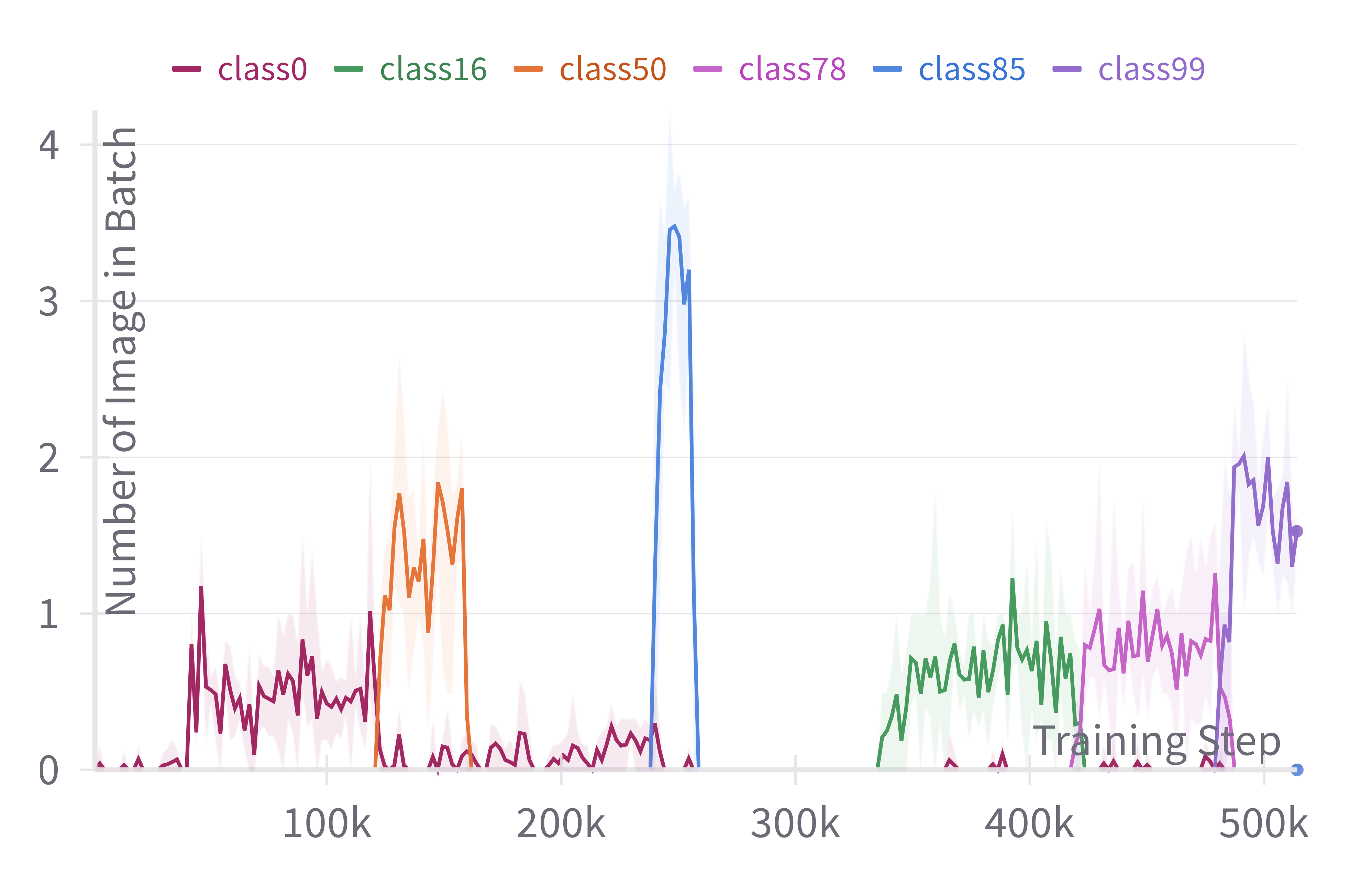
We followed the procedure and code made available by the authors of MVP (Moon et al., 2023) in order to generate the Si-Blurry versions of the datasets. Notably, we use and , following the original work. The number of tasks is the same as in the clear setting. We show the number of images per class apparition during training for a subset of classes to give a better overview of this training environment in Figure 5.
| Dataset | CIFAR100 | Imagenet-R | CUB | |||||||||
|---|---|---|---|---|---|---|---|---|---|---|---|---|
| Learning Rate | Avg. | Avg. | Avg. | |||||||||
| L2P | 66.88±0.48 | 69.75±1.75 | 59.74±0.74 | 65.46±0.99 | 45.16±1.13 | 47.24±1.86 | 26.68±2.31 | 39.69±1.77 | 36.39±3.12 | 39.2±1.75 | 17.81±1.11 | 31.13±1.99 |
| + OP | 72.19±0.11 | 79.54±0.39 | 73.98±0.64 | 75.24±0.38 | 52.81±0.71 | 63.42±0.29 | 46.13±0.19 | 54.12±0.4 | 60.67±2.3 | 75.11±2.46 | 46.95±2.51 | 60.91±2.42 |
| + CWH | 73.33±0.47 | 79.36±0.32 | 74.92±0.7 | 75.87±0.5 | 52.46±1.09 | 63.15±0.28 | 49.17±0.35 | 54.93±0.57 | 60.25±3.23 | 75.06±1.8 | 56.4±1.52 | 63.9±2.18 |
| DualPrompt | 62.16±1.59 | 69.41±1.33 | 54.57±0.68 | 62.05±1.2 | 40.94±6.68 | 51.06±1.14 | 24.5±1.17 | 38.83±3.0 | 35.07±3.39 | 47.61±2.84 | 21.77±0.71 | 34.82±2.31 |
| + OP | 67.04±2.75 | 79.9±0.25 | 72.06±1.01 | 73.0±1.34 | 40.77±4.7 | 61.84±0.42 | 48.46±0.59 | 50.36±1.9 | 52.53±3.32 | 78.53±0.61 | 57.34±0.7 | 62.8±1.54 |
| + CWH | 64.62±2.29 | 79.43±0.48 | 73.2±1.07 | 72.42±1.28 | 43.99±6.43 | 61.25±0.27 | 52.08±0.64 | 52.44±2.45 | 51.01±5.05 | 78.89±0.94 | 65.7±0.66 | 65.2±2.22 |
| CODA | 61.63±3.44 | 75.25±1.87 | 67.68±1.08 | 68.19±2.13 | 26.51±1.21 | 55.25±2.49 | 27.56±0.97 | 36.44±1.56 | 20.82±12.31 | 47.92±1.96 | 22.56±0.52 | 30.43±4.93 |
| + OP | 67.47±4.36 | 79.53±0.72 | 82.01±0.28 | 76.34±1.79 | 35.44±4.43 | 64.76±5.24 | 54.87±0.78 | 51.69±3.48 | 40.98±12.96 | 73.73±2.23 | 55.87±0.47 | 56.86±5.22 |
| + CWH | 69.1±0.43 | 80.13±1.85 | 82.89±0.41 | 77.37±0.9 | 33.61±2.56 | 61.62±4.91 | 58.93±0.84 | 51.39±2.77 | 43.91±6.46 | 74.2±1.83 | 64.8±0.43 | 60.97±2.91 |
| ConvPrompt | 69.07±0.69 | 79.13±0.97 | 70.83±0.95 | 73.01±0.87 | 14.48±24.17 | 59.45±2.73 | 32.26±2.92 | 35.4±9.94 | 0.4±0.09 | 56.56±2.67 | 29.66±0.22 | 28.87±0.99 |
| + OP | 77.45±2.63 | 86.14±0.26 | 84.12±0.57 | 82.57±1.15 | 16.99±29.14 | 70.15±0.81 | 57.69±0.98 | 48.28±10.31 | 0.4±0.11 | 79.58±1.78 | 57.38±1.56 | 45.79±1.15 |
| + CWH | 79.89±3.74 | 85.69±0.41 | 84.78±0.64 | 83.45±1.6 | 33.93±28.98 | 66.77±2.36 | 57.38±1.03 | 52.69±10.79 | 61.89±13.97 | 75.64±3.33 | 66.29±0.85 | 67.94±6.05 |
| MVP | 27.37±1.99 | 40.58±1.61 | 33.85±5.76 | 33.93±3.12 | 21.61±1.2 | 30.12±0.24 | 27.23±0.66 | 26.32±0.7 | 13.02±1.74 | 28.58±2.76 | 26.36±0.53 | 22.65±1.68 |
| + OP | 46.0±2.88 | 80.0±0.47 | 75.83±3.94 | 67.28±2.43 | 26.63±2.05 | 55.48±0.91 | 55.83±0.29 | 45.98±1.08 | 40.77±1.59 | 80.13±0.53 | 71.78±1.34 | 64.23±1.15 |
| + CWH | 51.06±2.45 | 79.82±0.2 | 76.61±3.43 | 69.16±2.03 | 33.52±5.59 | 55.56±0.97 | 56.53±0.33 | 48.54±2.3 | 44.84±4.68 | 79.19±0.13 | 74.03±1.0 | 66.02±1.94 |
| Dataset | CIFAR100 | Imagenet-R | CUB | |||||||||
|---|---|---|---|---|---|---|---|---|---|---|---|---|
| Learning Rate | Avg. | Avg. | Avg. | |||||||||
| L2P | 65.74±0.46 | 70.09±1.44 | 62.66±3.44 | 66.16±1.78 | 46.39±0.84 | 38.78±14.14 | 29.02±1.39 | 38.06±5.46 | 40.09±0.78 | 41.25±0.93 | 23.24±1.1 | 34.86±0.94 |
| + OP | 74.77±0.29 | 80.15±1.05 | 74.0±0.77 | 76.31±0.7 | 52.9±2.59 | 62.78±0.6 | 47.12±1.22 | 54.27±1.47 | 60.54±2.97 | 74.97±0.83 | 48.95±0.85 | 61.49±1.55 |
| + CWH | 75.16±0.91 | 79.68±1.13 | 74.74±0.64 | 76.53±0.89 | 51.18±0.53 | 62.37±0.54 | 49.92±0.71 | 54.49±0.59 | 56.9±4.2 | 74.97±1.02 | 58.34±0.26 | 63.4±1.83 |
| DualPrompt | 62.23±0.55 | 71.36±0.73 | 57.53±0.36 | 63.71±0.55 | 41.69±7.76 | 50.31±2.65 | 26.86±1.11 | 39.62±3.84 | 39.36±3.86 | 49.29±3.72 | 25.74±1.58 | 38.13±3.05 |
| + OP | 70.49±2.71 | 80.11±0.21 | 72.68±1.98 | 74.43±1.63 | 43.2±5.4 | 62.07±0.6 | 50.17±1.4 | 51.81±2.47 | 56.67±4.01 | 78.92±1.08 | 59.76±1.12 | 65.12±2.07 |
| + CWH | 70.0±1.64 | 79.46±0.34 | 73.58±1.68 | 74.35±1.22 | 39.75±5.28 | 60.92±0.36 | 53.54±1.32 | 51.4±2.32 | 55.87±2.7 | 79.3±1.3 | 68.04±1.48 | 67.74±1.83 |
| CODA | 61.87±1.35 | 75.78±1.11 | 69.54±0.14 | 69.06±0.87 | 27.87±9.2 | 58.1±0.18 | 31.14±1.26 | 39.04±3.55 | 38.86±4.27 | 50.82±2.12 | 28.99±1.01 | 39.56±2.47 |
| + OP | 74.47±1.39 | 82.53±1.69 | 82.59±0.33 | 79.86±1.14 | 31.5±11.37 | 66.45±0.64 | 56.67±1.13 | 51.54±4.38 | 50.88±6.34 | 74.68±2.02 | 60.91±0.02 | 62.16±2.79 |
| + CWH | 74.03±0.74 | 82.5±1.76 | 83.36±0.39 | 79.96±0.96 | 37.6±0.97 | 63.65±3.45 | 59.69±1.04 | 53.65±1.82 | 50.95±4.63 | 74.06±1.17 | 68.8±0.94 | 64.6±2.25 |
| ConvPrompt | 45.37±38.07 | 80.02±0.39 | 74.57±1.54 | 66.65±13.33 | 12.72±21.2 | 59.98±1.18 | 35.48±2.65 | 36.06±8.34 | 37.63±2.61 | 54.71±5.95 | 34.51±3.02 | 42.28±3.86 |
| + OP | 79.37±0.7 | 87.07±0.89 | 84.48±1.24 | 83.64±0.94 | 31.29±27.08 | 71.08±0.9 | 58.49±3.31 | 53.62±10.43 | 8.2±13.32 | 79.93±1.42 | 64.74±0.68 | 50.96±5.14 |
| + CWH | 80.97±1.61 | 86.67±1.09 | 84.16±1.51 | 83.93±1.4 | 35.68±29.53 | 69.36±1.03 | 56.97±3.83 | 54.0±11.46 | 67.4±3.0 | 78.17±6.07 | 70.64±1.17 | 72.07±3.41 |
| MVP | 32.8±6.71 | 48.33±3.44 | 40.54±2.18 | 40.56±4.11 | 23.25±4.73 | 31.64±0.87 | 29.04±0.99 | 27.98±2.2 | 19.07±2.05 | 33.45±1.62 | 27.89±1.44 | 26.8±1.7 |
| + OP | 49.37±3.54 | 81.38±0.63 | 76.62±0.64 | 69.12±1.6 | 27.99±11.28 | 57.53±0.4 | 56.56±0.24 | 47.36±3.97 | 44.53±6.4 | 80.66±0.71 | 73.64±1.23 | 66.28±2.78 |
| + CWH | 52.51±4.18 | 81.07±0.71 | 77.11±0.7 | 70.23±1.86 | 33.84±2.58 | 57.47±0.65 | 57.18±0.36 | 49.5±1.2 | 45.7±11.3 | 80.51±2.1 | 76.32±1.5 | 67.51±4.97 |
| Dataset | CIFAR100 | Imagenet-R | CUB | |||||||||
|---|---|---|---|---|---|---|---|---|---|---|---|---|
| Learning Rate | Avg. | Avg. | Avg. | |||||||||
| L2P | 64.81±0.78 | 68.49±2.81 | 58.48±1.74 | 63.93±1.78 | 44.21±1.3 | 46.78±1.96 | 26.29±1.8 | 39.09±1.69 | 34.69±2.71 | 38.0±1.24 | 17.76±0.18 | 30.15±1.38 |
| + OP | 70.16±0.3 | 79.05±1.15 | 75.6±1.17 | 74.94±0.87 | 51.88±0.81 | 63.49±0.19 | 47.51±0.12 | 54.29±0.37 | 59.48±2.8 | 75.42±1.74 | 48.84±2.41 | 61.25±2.32 |
| + CWH | 71.21±0.82 | 78.74±1.07 | 76.29±1.23 | 75.41±1.04 | 51.51±1.24 | 63.19±0.46 | 50.57±0.23 | 55.09±0.64 | 59.27±3.19 | 75.66±1.22 | 58.99±1.32 | 64.64±1.91 |
| DualPrompt | 59.46±1.03 | 67.76±1.84 | 53.06±1.24 | 60.09±1.37 | 39.3±7.18 | 50.7±0.94 | 24.42±1.15 | 38.14±3.09 | 33.27±3.24 | 46.71±2.59 | 21.12±0.94 | 33.7±2.26 |
| + OP | 64.64±3.07 | 79.69±0.4 | 73.89±1.21 | 72.74±1.56 | 39.04±4.91 | 61.83±0.25 | 50.11±0.67 | 50.33±1.94 | 50.85±3.05 | 78.56±0.47 | 59.21±0.96 | 62.87±1.49 |
| + CWH | 61.75±2.5 | 78.99±0.47 | 74.83±1.18 | 71.86±1.38 | 42.41±6.84 | 61.14±0.34 | 53.62±0.65 | 52.39±2.61 | 49.65±5.22 | 79.04±0.7 | 67.91±1.08 | 65.53±2.33 |
| CODA | 59.93±2.72 | 73.64±2.47 | 65.72±1.64 | 66.43±2.28 | 25.42±1.26 | 54.4±2.67 | 26.85±0.98 | 35.56±1.64 | 18.88±12.78 | 46.51±1.9 | 21.84±0.65 | 29.08±5.11 |
| + OP | 64.93±4.38 | 78.08±1.16 | 81.58±0.37 | 74.86±1.97 | 34.38±4.77 | 64.21±5.79 | 56.14±0.52 | 51.58±3.69 | 39.67±13.24 | 73.15±2.29 | 57.89±0.61 | 56.9±5.38 |
| + CWH | 66.42±0.3 | 78.8±2.36 | 82.56±0.8 | 75.93±1.15 | 31.61±3.21 | 61.02±5.09 | 60.07±0.6 | 50.9±2.97 | 42.06±7.08 | 73.91±2.31 | 67.19±0.98 | 61.05±3.46 |
| ConvPrompt | 67.2±0.46 | 77.77±1.07 | 69.11±0.44 | 71.36±0.66 | 14.03±23.53 | 58.72±2.96 | 31.61±2.77 | 34.79±9.75 | 0.31±0.27 | 55.56±2.51 | 29.27±1.17 | 28.38±1.32 |
| + OP | 75.96±3.12 | 85.49±0.57 | 83.37±0.61 | 81.61±1.43 | 16.58±28.41 | 69.89±1.09 | 58.13±0.99 | 48.2±10.16 | 0.1±0.18 | 79.18±1.82 | 59.03±1.76 | 46.1±1.25 |
| + CWH | 78.54±4.24 | 84.88±0.63 | 84.26±0.44 | 82.56±1.77 | 32.92±28.63 | 66.31±2.56 | 58.6±1.13 | 52.61±10.77 | 60.58±14.61 | 75.0±3.08 | 69.01±0.87 | 68.2±6.19 |
| MVP | 19.82±1.99 | 34.39±1.73 | 27.47±6.2 | 27.23±3.31 | 18.19±1.73 | 26.99±0.9 | 25.3±0.72 | 23.49±1.12 | 8.74±1.9 | 24.91±2.98 | 24.36±1.16 | 19.34±2.01 |
| + OP | 40.51±3.49 | 78.72±1.0 | 75.12±4.79 | 64.78±3.09 | 23.42±1.99 | 53.73±1.23 | 55.23±0.49 | 44.13±1.24 | 37.8±2.03 | 79.27±0.71 | 71.69±1.99 | 62.92±1.58 |
| + CWH | 46.15±2.57 | 78.54±0.81 | 75.81±4.27 | 66.83±2.55 | 30.81±6.23 | 53.82±1.22 | 55.62±0.53 | 46.75±2.66 | 42.18±4.9 | 78.28±0.11 | 73.5±1.51 | 64.65±2.17 |
| Dataset | CIFAR100 | Imagenet-R | CUB | |||||||||
|---|---|---|---|---|---|---|---|---|---|---|---|---|
| Learning Rate | Avg. | Avg. | Avg. | |||||||||
| L2P | 65.74±0.46 | 70.09±1.44 | 62.66±3.44 | 66.16±1.78 | 46.39±0.84 | 38.78±14.14 | 29.02±1.39 | 38.06±5.46 | 40.09±0.78 | 41.25±0.93 | 23.24±1.1 | 34.86±0.94 |
| + OP | 74.77±0.29 | 80.15±1.05 | 74.0±0.77 | 76.31±0.7 | 52.9±2.59 | 62.78±0.6 | 47.12±1.22 | 54.27±1.47 | 60.54±2.97 | 74.97±0.83 | 48.95±0.85 | 61.49±1.55 |
| + CWH | 75.16±0.91 | 79.68±1.13 | 74.74±0.64 | 76.53±0.89 | 51.18±0.53 | 62.37±0.54 | 49.92±0.71 | 54.49±0.59 | 56.9±4.2 | 74.97±1.02 | 58.34±0.26 | 63.4±1.83 |
| DualPrompt | 62.23±0.55 | 71.36±0.73 | 57.53±0.36 | 63.71±0.55 | 41.69±7.76 | 50.31±2.65 | 26.86±1.11 | 39.62±3.84 | 39.36±3.86 | 49.29±3.72 | 25.74±1.58 | 38.13±3.05 |
| + OP | 70.49±2.71 | 80.11±0.21 | 72.68±1.98 | 74.43±1.63 | 43.2±5.4 | 62.07±0.6 | 50.17±1.4 | 51.81±2.47 | 56.67±4.01 | 78.92±1.08 | 59.76±1.12 | 65.12±2.07 |
| + CWH | 70.0±1.64 | 79.46±0.34 | 73.58±1.68 | 74.35±1.22 | 39.75±5.28 | 60.92±0.36 | 53.54±1.32 | 51.4±2.32 | 55.87±2.7 | 79.3±1.3 | 68.04±1.48 | 67.74±1.83 |
| CODA | 61.87±1.35 | 75.78±1.11 | 69.54±0.14 | 69.06±0.87 | 27.87±9.2 | 58.1±0.18 | 31.14±1.26 | 39.04±3.55 | 38.86±4.27 | 50.82±2.12 | 28.99±1.01 | 39.56±2.47 |
| + OP | 74.47±1.39 | 82.53±1.69 | 82.59±0.33 | 79.86±1.14 | 31.5±11.37 | 66.45±0.64 | 56.67±1.13 | 51.54±4.38 | 50.88±6.34 | 74.68±2.02 | 60.91±0.02 | 62.16±2.79 |
| + CWH | 74.03±0.74 | 82.5±1.76 | 83.36±0.39 | 79.96±0.96 | 37.6±0.97 | 63.65±3.45 | 59.69±1.04 | 53.65±1.82 | 50.95±4.63 | 74.06±1.17 | 68.8±0.94 | 64.6±2.25 |
| ConvPrompt | 45.37±38.07 | 80.02±0.39 | 74.57±1.54 | 66.65±13.33 | 12.72±21.2 | 59.98±1.18 | 35.48±2.65 | 36.06±8.34 | 37.63±2.61 | 54.71±5.95 | 34.51±3.02 | 42.28±3.86 |
| + OP | 79.37±0.7 | 87.07±0.89 | 84.48±1.24 | 83.64±0.94 | 31.29±27.08 | 71.08±0.9 | 58.49±3.31 | 53.62±10.43 | 8.2±13.32 | 79.93±1.42 | 64.74±0.68 | 50.96±5.14 |
| + CWH | 80.97±1.61 | 86.67±1.09 | 84.16±1.51 | 83.93±1.4 | 35.68±29.53 | 69.36±1.03 | 56.97±3.83 | 54.0±11.46 | 67.4±3.0 | 78.17±6.07 | 70.64±1.17 | 72.07±3.41 |
| MVP | 32.8±6.71 | 48.33±3.44 | 40.54±2.18 | 40.56±4.11 | 23.25±4.73 | 31.64±0.87 | 29.04±0.99 | 27.98±2.2 | 19.07±2.05 | 33.45±1.62 | 27.89±1.44 | 26.8±1.7 |
| + OP | 49.37±3.54 | 81.38±0.63 | 76.62±0.64 | 69.12±1.6 | 27.99±11.28 | 57.53±0.4 | 56.56±0.24 | 47.36±3.97 | 44.53±6.4 | 80.66±0.71 | 73.64±1.23 | 66.28±2.78 |
| + CWH | 52.51±4.18 | 81.07±0.71 | 77.11±0.7 | 70.23±1.86 | 33.84±2.58 | 57.47±0.65 | 57.18±0.36 | 49.5±1.2 | 45.7±11.3 | 80.51±2.1 | 76.32±1.5 | 67.51±4.97 |