Operator size growth in Lindbladian SYK
Abstract
We investigate the growth of operator size in the Lindbladian Sachdev-Ye-Kitaev model with -body interaction terms and linear jump terms at finite dissipation strength. We compute the operator size as well as its distribution numerically at finite and analytically at large . With dissipative (productive) jump terms, the size converges to a value smaller (larger) than half the number of Majorana fermions. At weak dissipation, the evolution of operator size displays a quadratic-exponential-plateau behavior. The plateau value is determined by the ratios between the coupling of the interaction and the linear jump term in the large limit. The operator size distribution remains localized in the finite size region even at late times, contrasting with the unitary case. Moreover, we also derived the time-independent orthogonal basis for operator expansion which exhibits the operator size concentration at finite dissipation. Finally, we observe that the uncertainty relation for operator size growth is saturated at large , leading to classical dynamics of the operator size growth with dissipation.
1 Introduction
The scrambling of quantum information describes how a local operator spreads out and eventually affects the degree of freedom of many-body system under evolution Lieb2004 ; Hayden:2007cs ; Sekino:2008scramblers , as measured by the out-of-time-ordering correlator (OTOC) larkin:1969quasiclassical ; Shenker:2013yza ; Roberts:2014localized ; PRXQuantum.5.010201 ; Roberts:2016wdl ; Shenker:2013black ; Hosur:2015channels ; Roberts:2014ifa ; Stanford:2015owe . Scrambling can be easily understood as the growth of the size of operators Roberts:2018operator ; Qi:2018quantum , as a result of the cumulative commutation between the operator and the Hamiltonian during time evolution. Operator size is determined by the distribution of the Heisenberg operator on a local operator basis and is linearly related to the OTOC between initially local operators Roberts:2014localized ; Qi:2018quantum ; Qi:2019rpi . Recently, Krylov complexity has also been employed to describe operator growth Parker:2018a ; Barbon:2019on ; Avdoshkin:2019trj ; Jian:2020qpp ; Rabinovici:2020operator ; Avdoshkin:2019trj ; Dymarsky:2019quantum ; Carrega:2020unveiling ; Kar:2021nbm ; Caputa:2021sib ; Dymarsky:2021bjq ; Rabinovici:2021qqt ; Muck:2022xfc ; Rabinovici:2022beu ; Bhattacharjee:2022vlt ; Bhattacharjee:2022ave ; Avdoshkin:2022xuw ; Alishahiha:2022anw ; Huh:2023jxt ; Tang:2023ocr ; Aguilar-Gutierrez:2023nyk ; Kundu:2023hbk ; Beetar:2023mfn ; Bhattacharyya:2023dhp ; Loc:2024oen ; Malvimat:2024vhr ; Bhattacharya:2024uxx 111 The Krylov complexity on the state version characterizes the spreading of the wave function in the Hilbert space Balasubramanian:2022tpr ; Balasubramanian:2022dnj ; Erdmenger:2023wjg ; Balasubramanian:2023kwd ; Camargo:2023eev ; Bhattacharyya:2023grv ; Caputa:2024vrn . , although the Krylov basis for operator expansion typically is not a set of local operators.
Scrambling is enhanced by strong coupling and exhibits universal behavior in chaotic systems, such as the Sachdev-Ye-Kitaev (SYK) model Kitaev:2015a ; Maldacena:2016remarks ; Roberts:2018operator ; Qi:2018quantum ; Lin:2023trc , random matrix theory Roberts:2016design ; Cotler:2017jue , random circuits Hosur:2015channels ; Nahum:2017operator ; vonKeyserlingk:2017operator ; Xu:2018locality , and black holes Shenker:2013black ; Roberts:2014localized ; Maldacena:2016conformal ; Lensky:2020size ; Mousatov:2019operator ; Lin:2019symmetries . In particular, in these models, the operator size was found to exhibit exponential growth, whose exponent saturates the chaos bound Maldacena:2015waa . In the SYK model, the scrambling time for the size of local operators scales as , with being the number of fermions Sekino:2008scramblers . Scrambling is suppressed by localization Fan:2016ean and dissipation Chen:2017dbb ; Zhang:2018oop .
Scrambling can be measured via forward and backward evolution Li:2016xhw ; Garttner:2016mqj ; Sanchez:2020LoschmidtEcho ; Sanchez:2022LoschmidtEchoNER ; Dominguez:2021decoherence ; Dominguez:2021keq ; Mi:2021gdf ; Cotler:2022fin ; Swingle:2016var , entangled double-copy systems Islam:2015mom ; Landsman:2018jpm ; Blok:2020may , or randomized measurements Brydges:2019probing ; Joshi:2020PRL ; Blocher:2023hvk . For a realistic experimental setup, the dynamics of an open system is inevitably affected by the environment and becomes fundamentally non-unitary. When the system is weakly coupled to a Markovian reservoir, its dynamics is described by the Lindbladian master equation breuer2002theory ; lidar2019lecture ; manzano2020short , which is equivalent to the dynamics on the double-copy Hilbert space governed by a non-Hermitian Hamiltonian Denisov:2018nif . For Markov processes, such as the Lindbladian spin chain Schuster:2022bot or the Lindbladian SYK model Kulkarni:2021gtt ; Kawabata:2022osw ; Garcia-Garcia:2022adg ; Sa:2021tdr ; Bhattacharjee:2023uwx at weak dissipation, the size for local operators exhibits growth-plateau behavior, which is determined by the competition between the unitary interaction and non-unitary dissipation. Similar plateau behaviors were observed in Krylov complexity Liu:2022god ; Bhattacharjee:2022lzy ; Bhattacharya:2022gbz ; Bhattacharjee:2023uwx ; Bhattacharya:2023zqt ; Bhattacharya:2023yec . For a non-Markov process, such as the Brownian SYK coupled to a bath Zhang:2023BrownianSize , the size can decay to zero for strong system-bath couplings.
In this work, our aim is to comprehensively understand the growth of operator size in the Lindbladian SYK, particularly through analytical methods based on the path integral and the large limit. By employing these analytical solutions, we explicitly compute quantities such as the Loschmidt echo fidelity, operator size, size distribution, and size variances, and determine their time scales across all parameter regions. Additionally, We also prove the operator size concentration of Krylov basis from the path integral perspective. Finally, we elucidate on the emergence of classical dynamical equations governing operator size growth Qi:2018quantum , which are frequently utilized in estimating operator size growth in open systems Schuster:2022bot .
In this paper, we numerically and analytically calculate the operator sizes and size distributions of Heisenberg operators in a Lindbladian SYK model with linear jump operators. In Sec. 2, we define operator size, express its generating function as a path integral, and study the symmetries of the two-point function. In Sec. 3, we adopt exact diagonalization (ED) at finite and , and numerically solve Schwinger-Dyson (SD) equations at infinite and finite . In Sec. 4, we analytically solve the Liouville equations at large and obtain complete information about the operator size growth in this limit. In Sec. 5, we derive a classical equation for operator size growth by noticing the saturation of a relative uncertainty relation. In Sec. 6, we conclude and give an outlook on future directions.
2 Lindbladian SYK
In this section, we first discuss the Linbladian SYK model and apply it to the Heisenberg evolution of operators. We further map the Linbladian superoperator onto a Liouvillian operator on the double copy Hilbert space, and define the operator size and its generating function. Later, we write the corresponding partition function in path integral along the contour in the double copy Hilbert space. Following known methods for the SYK model, we obtain the effective action and the Schwinger-Dyson equation. In the last part, we find the symmetries of the two-point functions based on the symmetries of the model.
2.1 Lindbladian
The Lindblad master equation, or Lindbladian, for a density matrix in the Schrödinger picture is
| (1) |
which is interpreted as a super-operator . The Lindbladian with can effectively describe the microscopic model for a system coupled to an environment (bath) in certain limits. On one hand, the Lindbladian can be derived in the weak coupling limit, where the system-bath coupling is weak compared to the characteristic energy scales of both the system and the bath. More precisely, the weak coupling limit encompasses the Born approximation, the Markov approximation, and the rotating wave approximation. On the other hand, the Lindbladian can also be derived in the singular coupling limit, where the bath Hamiltonian dominates over the system Hamiltonian and the system-bath interaction breuer2002theory ; lidar2019lecture ; manzano2020short . Therefore, we will not assume any hierarchy between the strengths of the two terms in the Lindbladian (1).
One can also write down the Lindbladian for an operator in the Heisenberg picture
| (2) |
where when any one of and is bosonic and when both are fermionic Liu:2022god . In Liu:2022god , the Lindbladian for an operator is derived by tracing out the Markovian bath and imposing the white noise approximation on the bath correlation in an integral equation of the unitary Heisenberg equation of the operator.
The Lindbladian itself is a consistent theory for any real value of , including , mathematically. We will provide an interpretation of the case where later in our Lindbladian SYK model. In this paper, we will use the Lindbladian in (2) as our starting point and will not consider its microscopic origin in the system-plus-bath composite system.
Both Lindbladians preserve the trace and the maximally mixed state, which is proportional to the identity, namely . When the Lindblad operators are Hermitian, , the two equations (1) and (2) are identical by mapping . It is exactly this case we consider in this paper, and we will adopt the Lindbladian in the Heisenberg picture (2) throughout out this paper. The first term describes the unitary evolution and the second term introduces the effect of physical non-unitary. The coefficient could be interpreted as the error rate of quantum gates in quantum circuits Schuster:2022bot .
In this paper, we consider an even number Majorana fermions , with anti-commutation relation . The Hamiltonian is taken to be the Sachdev-Ye-Kitaev (SYK) model Kitaev:2015a ; Maldacena:2016remarks
| (3) |
with even number and . The Lindblad operators are taken as the linear jump operators Kulkarni:2021gtt
| (4) |
The dimension of Hilbert space is . To derive the Lindbladian with linear jump operators, one could couple the SYK system with a Markovia bath, where the bath correlation follows white noise approximation , the hopping term is and is the Majorana fermion of the bath Liu:2022god . Last but not least, the Lindbladian SYK model we consider in this paper is theoretically well-defined completely positive trace preserving map for all the parameters , although is still debatable whether one can find the original from a microscopic dynamics.
Following Qi:2018quantum ; Kulkarni:2021gtt , we will use the Choi-Jamiolkowski isomorphism with the double-copy Hilbert space and Majorana fermions satisfying with . Following (3), we use to construct and use to construct . Given a bosonic (fermionic) operator acting on , we can construct two bosinic (fermionic) operators () acting on where Hermitian operator . One can check that () for any bosonic (fermionic) linear operator .
We define a maximally entangled state in as
| (5) |
One can check that . The maximally entangled state induces a map from a linear operator acting on the single Hilbert space to a state in the double-copy Hilbert space via
| (6) |
Then the identity acting on is mapped to . The operator trace in is mapped to the inner product in via .
The Lindbladian is mapped to a non-Hermitian Liouvillian
| (7) |
acting on via , where
| (8) |
is called the size operator, whose meaning will be explained in the next subsection. The factor in (2) is canceled out in (7) when and are exchanged. At the last step of (7), we decompose the Liouvillian into anti-Hermitian part and Hermitian part . Thus, One can check that . The Liouvillian is reminiscent of the Hamiltonian for eternal traversable wormhole Gao:2016bin ; Maldacena:2018lmt ; Milekhin:2022bzx with the same second term, but here the Hamiltonians on each side have the opposite signs.
2.2 Operator size
To study the information scrambling in the Lindbladian SYK model, we introduce the operator size following Qi:2018quantum . First, we define a local, complete, operator basis acting on , consisting of Majorana strings, namely
| (9) |
with notation , where the factor is introduced to make Hermitian. The basis is orthogonal and normalized under the inner product . The basis is complete since the number of elements is equal to the square of the dimension of Hilbert space , even in the limit. Second, we define the size superoperator so that it is diagonal on the Majorana strings basis with the eigenvalues measuring the numbers of Majorana fermions
| (10) |
which defines the size of all the linear operators acting on . Obviously, the identity has smallest size and has largest size .
Based on the mapping (6) to the double-copy Hilbert space , the assignment (10) simply corresponds to the size operator defined in (8), as one can check from the eigensystem and diagonalization . Obviously, and we denote . We define the size subspace and its projection operator
| (11) |
The dimension of is . The size operator can be expanded as . The Lindblad term in (7) with () suppresses (enhances) eigenstates with large sizes. So, we refer to the effect induced by the Lindblad term with as dissipation, and that with as production. One can measure the size of any operator acting on by the size operator
| (12) |
with the size operator in (8) and
| (13) |
the generating function of the operator size Qi:2018quantum . The generating function also gives the size distribution via
| (14) |
where the distribution is normalized as .
For the sake of analytic solvability, in the main text of this paper, we focus on the case of in the Heisenberg picture and calculate the size and the generating function
| (15) |
Obviously, for all even . So , in contrast to the case of a non-Markovian reservoir Zhang:2023BrownianSize . In the App. B, we consider two initial operators and and numerically study their sizes under the Lindbladian evolution. For later convenience, we further introduce the double-time generating function
| (16) |
It is the transition amplitude between the states at two different times and under the influence of the insertion . Obviously, .
The operator size for small enough was studied in Schuster:2022bot semi-classically, and also calculated in the same limit in Bhattacharjee:2023uwx from the Krylov complexity perspective. Here, we are able to solve this problem for any value of numerically at finite and analytically at large , so that we can investigate the operator size and distribution dynamics in the Lindbladian SYK model at finite dissipation or production and observe fast saturation of the size and the distribution.
2.3 Path integral

We will utilize the path integral to calculate the generating function of size (15). Let us consider the partition function
| (17) |
Since , we know that for any . So we are free to choose any and in (17). Furthermore, the two-point function should be independent of the choice of since and . On the r.h.s. of (17), we write the partition function as the path integral of two real Grassmann fields along the double-copy contour in Fig. 1 with Garcia-Garcia:2022adg ; Kawabata:2022osw . The action is
| (18) |
where and are functions of real Grassmann variables in the forms of (3) and (8). Notice that the unusual sign function before the Hamiltonians originates from the piecewise evolution along the contour. The term corresponds to the insertion of at . Due to the initial and final state (5), the path integral is subjected to the boundary conditions
| (19) |
As in the pure SYK model Maldacena:2016remarks , we take the disorder average, keep the dominating replica diagonal part and obtain the action
| (20) |
where comes from the disorder average between two different locations and is defined as
| (21) |
We introduce the bi-local fields
| (22) |
and via the Lagrange multiplier method
| (23) |
By integrating out the Grassmann variables , we obtain the effective action for bi-local fields
| (24) |
The boundary condition (19) becomes
| (25) |
In the large limit, by taking the variation on the bi-local fields, we obtain the Schwinger-Dyson (SD) equation
| (26a) | |||
| (26b) | |||
where and . The on-shell solution should be independent of and , such that the boundary condition (25) actually holds for any . This fact leads to the following simplification:
| (27) |
where . To establish similar relations between the components of the self energy, we need to isolate the contribution from the anti-symmetric term in (26b) by defining , which follows the same relations as (27), namely
| (28) |
So, only one of the four components in and are independent. We choose and , and simplify the SD equations as
| (29a) | ||||
| (29b) | ||||
such that and disappear. Now the equation is real, so we expect real solutions of and . Other components could be reconstructed via (27) and (28).
The two-point function derived from the path integral, or from solving the SD equation (26) in the large limit, can be expressed as the following expectation value
| (30) |
where the operator evolution is defined as
| (31) |
and the time ordering compatible with the path integral (17) and (2.3) is
| (32) |
with if both operators are fermionic, and in other cases. Under the disorder average, the generating functions (15)(16) will not depend on the choice of the Majorana index and equals the specific two-point function
| (33) |
where .
2.4 Symmetries
The factor in the path integral (2.3) divides the time domain into two parts and . So, the double-time argument in has distinct cases. Besides the relationship (27) between the components of , we should further identify the independent time domain in based on other symmetries.
We will review some transformations and symmetries in the -symmetric Linbladian Prosen:2012sn ; Garcia-Garcia:2023yet . They will provide us with the symmetries of the spectrum and the symmetries of the two-point function, which connect the two-point function in different time domains.
-
•
Anti-commutation relation of fermions. Exchanging the and in (30) leads to the relation
(34) -
•
Hermitian conjugation . Since , the conjugate of the two-point function will change the time argument,
(35) -
•
Parity and time reversal . They are defined as
(36) where we have expressed the transformation acting on the representation of Majorana fermions of the Jordan–Wigner (JW) transformation,
(37) in this representation performs the complex conjugation of a matrix. The action of transformations are listed in Tab. 1. One can check that and the Liouvillian has symmetry
(38) The symmetry ensures that the spectrum of is invariant under conjugation Bender:1998PT ; Mostafazadeh:2001jk ; Mostafazadeh:2001nr ; Mostafazadeh:2002id ; Zhang:2019gyc ; Prosen:2012sn . Combining the transformation, we have the relation
(39) where .
Table 1: The transformation of some operators under and . -
•
transformation. It is defined as Garcia-Garcia:2023yet
(40) with and . Some results of transformation are listed in Tab. 1. The particle-hole conjugation is Cotler:2016fpe . We can check that
(41) So the spectrum of is symmetric respective to the origin. Since does not preserve the state , it can not be a new symmetry of the two-point function. However, it can relate the two-point function defined on state (30) and the following two-point function defined on state
(42) where is used. The relation between two-point functions results in a simple relation between two sizes
(43) Similarly, for the other operators, we will have , where is the complement of . This relation aligns with our intuition: a jump term in the Linbladian with strength , which suppresses the size of , has the same effect as the jump term with that enhances the size of . In this sense, the Lindbladian with is also meaningful for the system coupled to a Markovian reservoir.
In summary, the spectrum of is symmetric with respect to both the real axis and the imaginary axis. The two-point function has the symmetries:
| (44) |
Combining them with the simplification (27), we can reduce the two-point function to a single component in an independent time domain. We choose
| (45) |
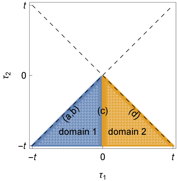
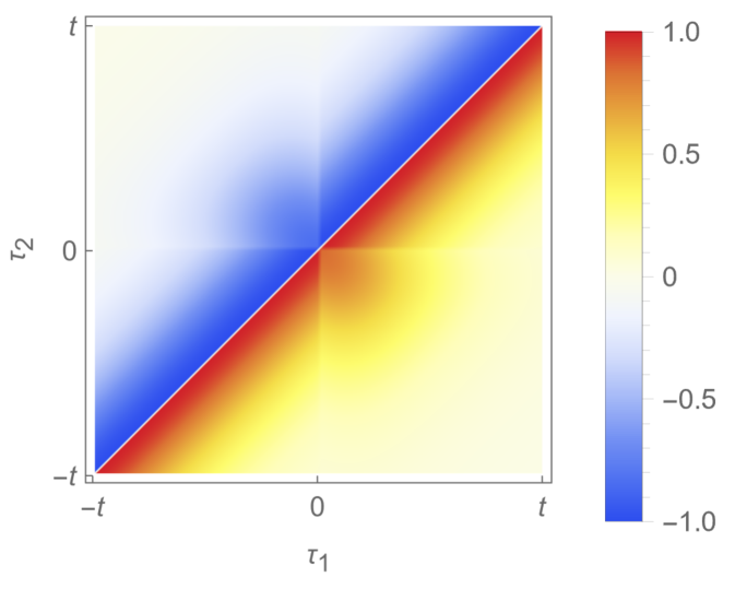
The time domain forms a triangle, as shown in Fig. 2. With this analysis on our hands, we will now numerically and analytically solve the problem in the following two sections.
3 Numerical operator size at finite
3.1 Exact diagonalization at finite

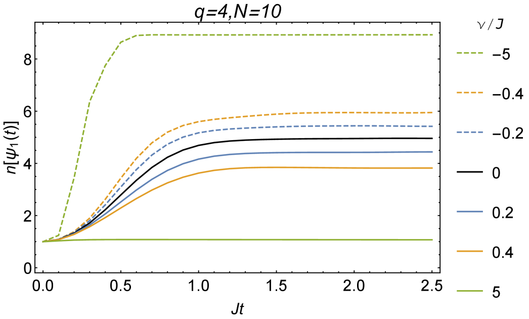
We will numerically diagonalize the Liouvillian (7) at and and then study the evolution of the operator size and size distribution. We observe that, when (), the operator size growth is suppressed (enhanced) and the size reaches a stable value smaller (bigger) than at the late time. We skip the case of , since the size is trivially .
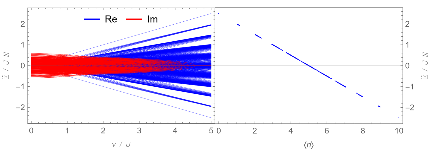
We use the Jordan-Wigner transformation (37) to construct the Liouvillian (7) and numerically diagonalize it to find its spectrum , see also Kulkarni:2021gtt ; Zhou:2021yyw . We plot the shifted spectrum , because it is symmetric with respect to both the real axis and the imaginary axis, according to the symmetry analysis in Subsec. 2.4. The spectrum of one realization at positive is shown in the left panel of Fig. 3, which is identical to the spectrum with . The spectrum of Liouvillian is quite different from the pure SYK spectrum Cotler:2016fpe ; Garcia-Garcia:2016mno ; you2017sachdev . When , the spectrum is real and exhibits energy bands and gaps, where the bands are approximately labeled by their sizes, as shown in the right panel of Fig. 3. When , some real energy pairs collide with each other and then move into the complex plane. The points where such collision happens are called exceptional points Bender:1998PT . When , most but not all the energies become complex.
We can further find the biorthogonal eigenbasis with and Brody2013BiorthogonalQM , except at the exceptional points, where two eigenstates become linearly dependent, . Before their collision, the two eigenstate have symmetry, namely and . After the collision, symmetry is spontaneously broken into . The real and imaginary parts of the spectrum are related to the decomposition of Liouvillian (7) via
| (46) |
or, equivalently, with being replaced.
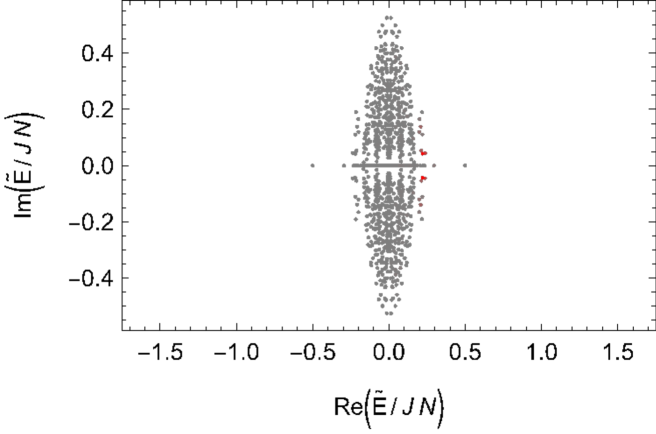
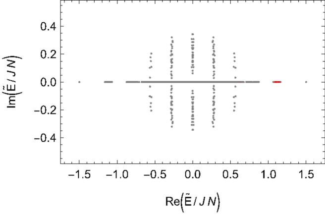
The spectrum and the probability distribution are plotted in Fig. 4. For a large , the energies exhibiting imaginary parts still form bands and gaps. The state mainly distributes around the band. When decreases, these bands collapse into a cluster. The state mainly distributes at the edge of the cluster with large . Based on the diagonalization and the probability distribution, we can calculate the size and size distribution
| (47) | ||||
| (48) |
where the normalization factor is determined by .
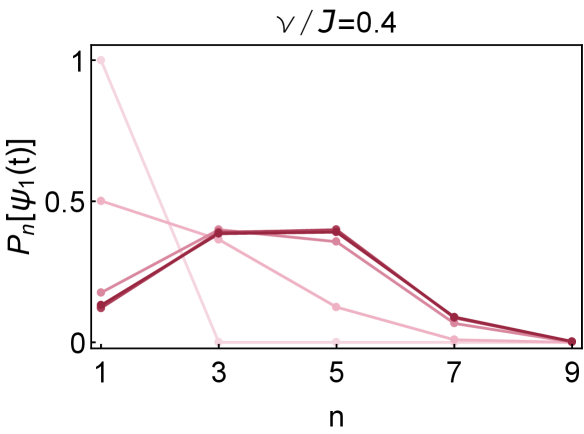
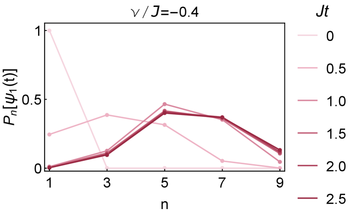
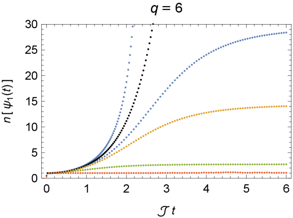
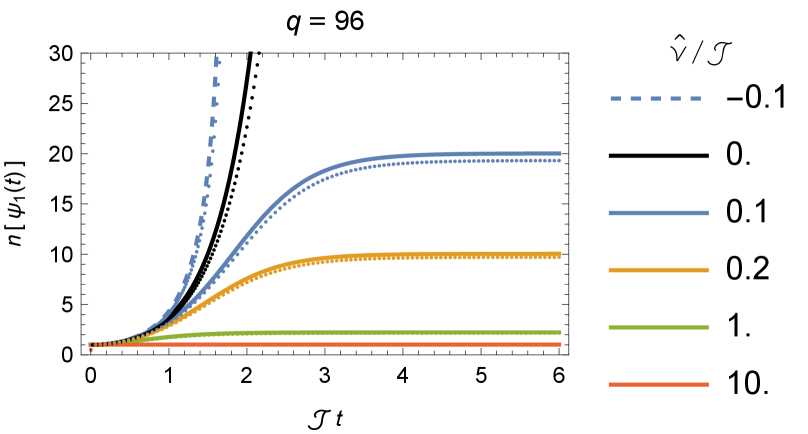
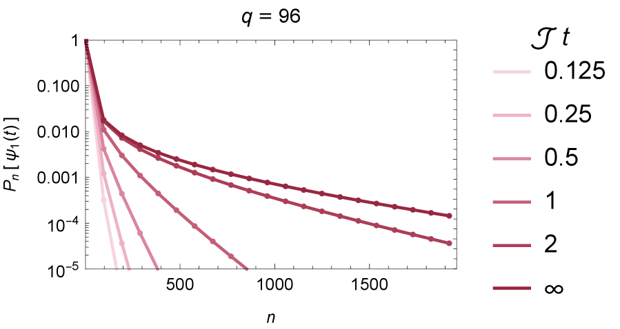
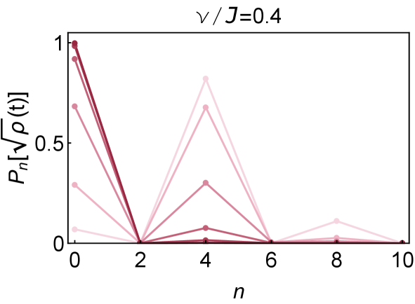
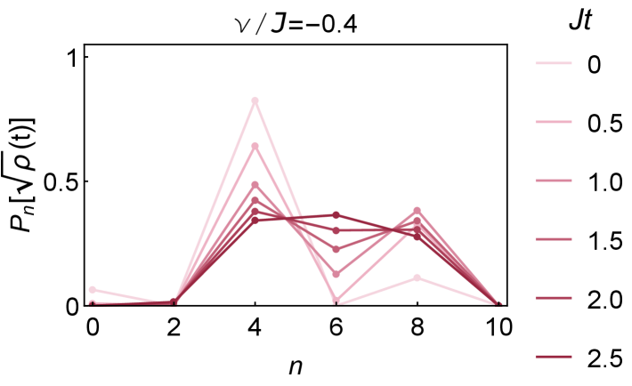
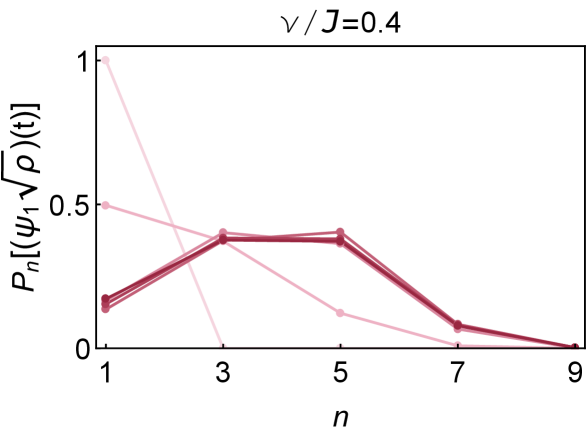
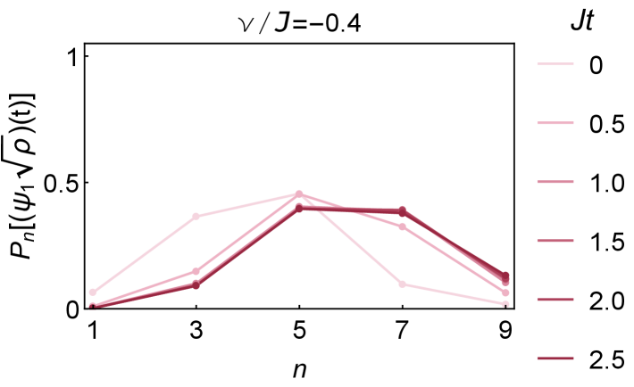
The growth of operator size from ED is shown in Fig. 5. The larger the , the slower the operator size grows, and the lower the plateau it reaches. But the reasons for the different sizes plateau of different varies. For , the plateau is given by due to full scrambling. With strong dissipation , the plateau is determined by the competition between the interaction and the dissipation . With strong production , the plateau is pushed to a value a small distance away from the maximally possible operator size , determined by the ratio between the interaction and the production . In the limit , the operator size will approach . In Fig. 6, we further show the size distribution for or . We can see that dissipation (production ) suppresses (enhances) the probability of large sizes. Notice that all the probability on even sizes vanish because each commutation with the SYK Hamiltonian can only change the size by even numbers.
In App. B, we calculate the size and size distribution of the pure SYK thermal state and the thermal fermion in the same way. For low temperature, these operators have larger initial sizes. Their sizes decrease or increase, depending on the strength of dissipation or production.
3.2 Numerical Schwinger-Dyson equation at infinite
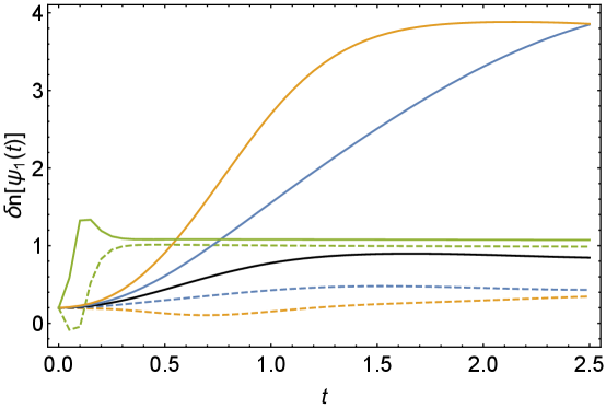
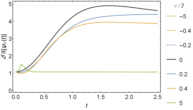
We also calculated the two-point function by numerically solving the SD equation (26). We plot the configurations of the numerical solution at finite in Fig. 7. Discontinuities appear across the interfaces and due to the insertion there. To extract the operator size according to (12), we vary around and calculate the difference of generating functions. We have chosen a long time so that, as shown in Fig. 8, the overall growth-plateau behavior of the operator size is covered. For dissipation , the growth rate is suppressed and a plateau of operator size emerges at finite time. For production , the growth rate is enhanced and the numerical method breaks down in finite time, indicating the divergence of operator size and necessitating the regularization by finite effects. In the next section, we will find the analytical operator size growth at large , which nicely matches the numerical result for any at large but finite , as already demonstrated in Fig. 8.
4 Analytical operator size at large
In this section, we will solve the Lindbladian SYK in the large limit, where the SD equations, represented as integral equations, reduce to the Liouville equations, which are differential equations. Following Maldacena:2016remarks ; Maldacena:2018lmt ; Qi:2018quantum ; Streicher:2019wek ; Kulkarni:2021gtt , when considering the limit, we will keep the following parameters fixed
| (49) |
We will analytically solve the Liouville equations with boundary conditions and calculate the generating functions, Loschmidt echo fidelity, operator size, size distribution, and the variances of the size operator and the Liouvillian.
4.1 Liouville equation
Owing to the symmetries (44), we use the following large ansatz for the independent parts of two-point function (45)
| (50) |
where the prefactors are determined by the free case.
Plugging (50) into the SD equation (26), utilizing the relation (27) and taking the large expansion, we find that the order is automatically solved, and the order gives rise to the Liouville equation. Because the factor in the SD equation changes its sign at , we should further divide the triangular domain (45) into two subdomains, as shown in Fig. 2, where the Liouville equations behave differently in respected interiors
| (51a) | ||||
| (51b) | ||||
is termed uncrossed function because it represents the correlation not crossing the point , while is termed crossed function because it represents the correlation crossing the point .
Next, we discuss the conditions on the boundaries of domains 1 and 2, namely , and , as labeled in Fig. 2, where and :
-
(a)
From the anti-commutation relation, we have , so
(52) - (b)
-
(c)
The insertion of yields the twisted boundary condition Qi:2018quantum ; Streicher:2019wek
(55) It leads to the following twisted condition for both two-point functions at
(56) and similar one for . The two-point function exhibits discontinuity across the interface and the interface, as shown in the numerical solution in Fig. 7. At large , where is small, the twisted boundary conditions decouple as shown at the last step of (56). It leads to the following boundary condition between the crossed and uncrossed functions at the interface between domain 1 and domain 2,
(57) - (d)
Below we summarize all the boundary conditions derived above:
| (59a) | ||||
| (59b) | ||||
| (59c) | ||||
| (59d) | ||||
4.2 Solution and generating functions
The Liouville equations (51) with boundary conditions (59) can determine the solution. Here we find a solution through the following analysis. For the uncrossed function in domain 1, the operators and in the partition function (17) are eliminated by observing . So the uncrossed function should be the same as the translational invariant solution in Kulkarni:2021gtt . Then we can determine the crossed function in domain 2 by matching the general solution of the Liouville equation in Gao:2019nyj to the boundary conditions (59) with the known uncrossed function . The analytical solution we find is
| (60a) | |||
| (60b) | |||
where the parameters and are determined by
| (61) |
In the following two limits of weak and strong dissipation, the two parameters approach
| weak dissipation | (62) | |||
| strong dissipation | (63) |
The large expansion below (50) is valid when both and are . When , they decay as for large time differences . The solution is valid when . When , suffers from a divergence along a line in domain 2 where the denominator in (60b) vanishes. The large solution is not applicable beyond that line, and necessitates regularization due to the finite effect. Fortunately, the validity region in time is, due to the large limit, extensive enough for our analysis of operator size.
4.3 Loschmidt echo fidelity
Before calculating observable, we investigate the state first. The generating function (64) at reduces to the (square root of) Loschmidt echo fidelity Yan:2019fbg ; Schuster:2022bot
| (66) |
It measures the return amplitude for the state , which has undergone a forward-backward evolution in the presence of the difference between the two Hamiltonians . Contrary to the typical Loschmidt echo Gorin:2006loschmidt ; Goussev:2012loschmidt , the difference in this case is non-Hermitian. The Loschmidt echo fidelity decays exponentially as
| (67) |
after a time
| (68) |
which indicates the time when the state becomes stable up to normalization. We call the plateau time since most of the observable will become stable after this time, such as the operator size Schuster:2022bot and the Krylov complexity Bhattacharjee:2022lzy . At weak dissipation , the plateau time reduces to
| (69) |
This plateau time is similar to the Ehrenfest time in the unitary chaotic evolution Gorin:2006loschmidt ; Goussev:2012loschmidt . Recall the scrambling time in many-body chaotic systems, indicating the time when the local information spread over the system’s degree of freedom Sekino:2008scramblers ; Roberts:2014localized ; Shenker:2013yza ; Maldacena:2015waa ; Maldacena:2016remarks . The plateau time could be comparable to the scrambling time if .
As predicted by Jalabert:2001decoherence and observed in Schuster:2022bot , at weak dissipation, the decay rate of the Loschmidt echo (67) depends on the pure SYK Hamiltonian coupling but not on the dissipation strength . While, at finite dissipation, the decay rate becomes dependent on . Furthermore, at large , due to the power in (66) and (67), the fidelity is of order at the plateau time, decays extremely slowly, and becomes significantly lower than only after the time .
The double-time generating function (65) at reduces to the overlap between the states at different times without normalization. We can examine the normalized overlap probability
| (70) |
which is close to when both . It means that the state remains nearly unchanged up to normalization long after the plateau time .
4.4 Size growth
We denote the expectation value of an operator in state as
.
Plugging the generating function (64) into (12), we obtain the operator size
| (71) |
In Fig. 8, we show the behavior of the size in the large limit.
For vanishing dissipation , we have and . The size reduces to the pure SYK case Roberts:2018operator .
For dissipation , we always have and the plateau value is . For weak dissipation with , the size at different time scales behaves as
| (72) |
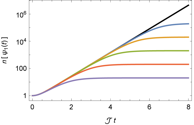
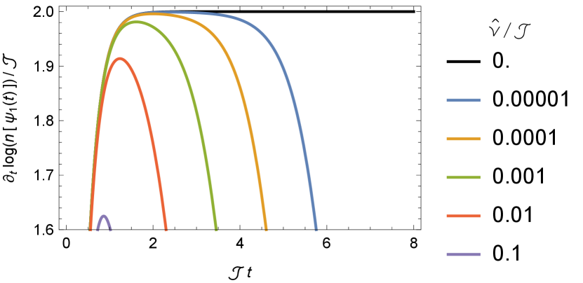
with the plateau time (68). So the dissipation reduces the growth rate as well as the plateau value. Only for weak dissipation , the hierarchy between and is huge enough for the emergence of an exponential growth region, as shown in Fig. 9. From (72), the leading correction resulting from dissipation in the exponential growth region breaks the pure exponential behavior rather than modifying its exponent. The plateau value approaches to at weak dissipation, as predicted in Schuster:2022bot . At strong dissipation , the size ceases to grow, .
4.5 Size distribution
To study the details of size growth, we calculate the size distribution. Expanding the generating function (64) according to (14) using the binomial theorem and normalizing the distribution, we obtain the size distribution
| (74) |
where
| (75) |
and for , due to the large- suppression of non-melonic diagrams and also the large limit Maldacena:2016remarks ; Gu:2016local ; Roberts:2018operator ; Qi:2018quantum . More precisely, the size with nonzero distribution should be , but the term is neglected in our discussion when considering large . We plot the distribution for in the left panel of Fig. 10.
When , the distribution in the long time limit converges to
| (76) |
Unlike the pure SYK case, for which Qi:2018quantum , once we have dissipation , the distribution is finite in the long time limit. The dissipation also leads to the exponential decay when is large enough.
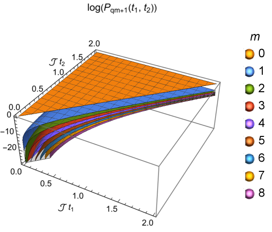
Similarly, we can expand the double-time generating function (65) according to
| (77) |
with normalization and get the double-time distribution
| (78) |
and for . It measures the overlap between and in the size subspace without state normalization. Its behavior is shown in the right panel of Fig. 10.
4.6 Operator size concentration
In this subsection, we prove the property of operator size concentration at finite dissipation in the large limit. The operator size concentration, proposed in Bhattacharjee:2022lzy ; Bhattacharjee:2023uwx , states that the state can be expanded on a time-independent and orthonormal , namely
| (79) |
where the -th basis state has size , i.e. with the size subspace (11). The statement is nontrivial, because has dimension and has to be localized in only one basis state in for all , where is the projection operator of the size subspace .
The operator size concentration was proved via constructing the basis from the (bi-)Lanczos algorithm in the large limit in Bhattacharjee:2022lzy ; Bhattacharjee:2023uwx . So the basis is called the Krylov basis and the coefficients is the Krylov wave function. Alternatively, in this work, we will prove the operator size concentration via the generating functions without constructing the Krylov basis from an iterative algorithm.
Because for , we can expand . So we expect . As we explained, the nontrivial task is to prove that is time-independent up to a normalization coefficient, in other words, to prove that and are linearly dependent for any . By using (70)(74)(78), we find that their normalized overlap in the size subspace automatically equals , namely
| (80) |
So we can simply choose the orthonormal basis state as
| (81) |
which is time-independent in the large limit. Thus, the basis with (81) satisfies all the above conditions of operator size concentration: time-independence, orthonormality, the ability to express , and each state belongs to a different size subspace, which concludes our proof.
From this point of view, the operator size distribution is actually the transition probability from to the orthonormal basis state under the Lindbladian evolution for time . So the Krylov wave function is
| (82) |
We further find that the wave function satisfies the discrete Schrödinger equation in the bi-Lanczos algorithm Bhattacharya:2023zqt ; Bhattacharjee:2023uwx
| (83) |
to the order of with the Lanczos coefficients
| (84) |
except for , where the overall factor in (74) needs a correction to fulfill the equation for at order. Thus, is the Krylov basis in the large- SYK model in Bhattacharjee:2022lzy . Due to the operator size concentration, the operator size is related to the Krylov complexity by
| (85) |
in the large limit. Also, we note that the operator size is proportional to the connected part of the OTOC or the square of anti-commutator normalized by the two-point function Roberts:2018operator ; Qi:2018quantum . It is derived via the double-time generating function (65) as
| (86) |
It can not be simply factorized into a form of at finite dissipation even and , in contrast to the Hermitian case Gu:2018jsv ; Gu:2021xaj 222We thank the authors of Garcia-Garcia:2024tbd for helpful discussion..
The Krylov complexity and the normalized square of anti-commutator were calculated in the same Lindbladian SYK model as ours in the first-order perturbation theory with respect to before, see (6.15) in Bhattacharjee:2022lzy and (7.21) in Bhattacharjee:2023uwx . As expected, their expressions coincide with our operator size in (71) at the leading-order in . Moreover, the square of the wave function in the Krylov space in (6.10) in Bhattacharjee:2022lzy also coincides with our size distribution (74) at the leading-order 333 We thank the authors of Bhattacharjee:2023uwx , especially Pratik Nandy, for helpful discussion and clarification. .
4.7 Variances
We further investigate the quantum fluctuations of the size operator and two terms in the Liouvillian in (7) by calculating their variances. We define the deviation of operator from its expectation value as . Using the generating function (64), we can calculate the size variance
| (87) |
where
| (88) |
When , vanishes.
The size variance is very big compared to because of the factor in (87) due to fluctuations generated by -body interactions. When , the relative variance approaches the long time limit
.
Using the double-time generating function (65), we can calculate the expectation values of some combinations between . The expectation values are given by
| (89) | ||||
| (90) | ||||
| (91) | ||||
| (92) |
The variances of the Liouvilian are
| (93) | ||||
| (94) | ||||
| (95) |
Notice that and always. When , and reduce to and respectively. When , they decay exponentially after the plateau time . The relative variance of Liouvillian is huge . The moment of Liouvillian can be constructed as .
Finally, we list some useful results for later convenience.
| (96) | |||
| (97) | |||
| (98) |
It is surprising that is independent of dissipation. Actually, we recognize as the Lanczos coefficient in (84). The balance between these quantum fluctuations is crucial for understanding the emergence of classical dynamics in the next section.
5 Emergence of classical size growth
In Qi:2018quantum ; Schuster:2022bot , the authors constructed classical equations to describe the dynamics of the operator size growth phenomenologically. Since we have nearly all the information about the operator size growth in this Lindbladian SYK at large , we can show that the emergence of classical dynamics of operator size growth is due to the saturation of the uncertainty relation of size growth in quantum mechanics.
Following Schuster:2022bot , the growth rate of can be written as
| (99) |
The first term is the unitary term, and the second term is the dissipation term. Since both and are Hermitian, they have the uncertainty relation
| (100) |
Similar uncertainty relations are applied in Hornedal:2022pkc ; Bhattacharya:2024uxx . Since the size (71) never decreases, the unitary term in (99) should be non-negative. This yields a limit on the growth rate
| (101) |
The uncertainty relation for the size operator and the Liouvillian is discussed in App. C.
The inequality (101) holds generically for the Liouvillian in the form of (7), independent of the microscopic details of the Hamiltonian . However, thanks to the large limit of the Lindbladian SYK, we can check this inequality by comparing (87), (96) and (98). We find that the uncertainty relation is actually saturated, namely
| (102) |
where . The saturation of the Cauchy-Schwarz inequality means that states and are linearly dependent. By calculating from the generating functions, we find that the linear coefficient is in (88), namely
| (103) |
So behaves like a coherent state of the time-dependent “annihilation operator” , which consists of the “position” operator and the “momentum” operator . The two operators follow the commutation relation in the bracket , and have the time-independent variances . From the asymptotic behavior of in (88), the operator interpolates between the size operator at early times and the Liouvillian at late times.
Coming back to the growth rate of the operator size, we find
| (104) | ||||
| (105) |
where
| (106) |
The first line (104) indicates that the size’s growth rate is controlled by its variance in quantum mechanics. Specifically, the larger the size variance, the more the operator will fail to commute with the Hamiltonian, but the dissipation also becomes larger in the meantime. In total, the growth rate of the size (104) is determined by this interplay. If we recognize the factor as the Lanczos coefficient in (84), then the first term in (104) could be identified as the saturated growth rate of Krylov complexity in Hornedal:2022pkc ; Bhattacharya:2024uxx .
In the second line (105), we derive the differential equation of operator size in Qi:2018quantum ; Schuster:2022bot . Following Qi:2018quantum , we could interpret (105) as the Susceptible-Infectious (SI) epidemic model with a stock of infected individuals , a contact rate , the total population , and no recovery. The total population in the SI model corresponds to an effective number of qubits in the Lindbladian SYK, controlling the steady state maximum operator size in (105), and taking the place of in the pure SYK case. At weak dissipation , the ratio converges to much after , which is still much early than the plateau time . So we can take the approximation in the differential equation (105), solve it with the initial condition , and find the solution valid in the region
| (107) |
It is close to the exact expression (71) at weak dissipation, including the time scales (72).
6 Conclusion and outlook
6.1 Conclusion
We comprehensively studied the operator size growth of a single Majorana fermion in the Lindbladian SYK model with a linear jump operator for both finite dissipation and finite production. The operator size and distribution can be derived from the two-point function with the insertion of in the path integral. The symmetries of the two-point function and the properties of the maximally entangled state greatly simplify the problem.
First, we used exact diagonalization to solve the model at finite and numerically solved the Schwinger-Dyson equation at infinite . We observed the slowdown (acceleration) of the operator size growth and the suppression (enhancement) of the size plateau due to the dissipation (production) introduced by the Lindblad terms with (). Second, we analytically solved the Liouville equations in the large limit and obtained the expression for the Loschmidt echo fidelity, operator size, size distribution, and the variances of size and the Liouvillian. The plateau time is extracted from the analytical results given. The operator size exhibits a quadratic-exponential-plateau behavior at weak dissipation and the size distribution is localized at finite size. Third, we construct the time-independent orthogonal basis exhibiting operator size concentration. Fourth, we derive a growth rate limit on the operator size from an uncertainty relation and find that it is saturated at large , which gives rise to classical dynamics of operator growth with dissipation. Five, we study the size of operators at finite temperature, including and , at finite in App. B.
We formulated a self-consistent path integral for studying operator size in Lindblad-ian dynamics. Our approach does not depend on the weak dissipation limit and can be readily extended to other fermionic models and Lindblad operators. We analytically derived the operator size and distribution of a single Majorana fermion, a feature that was previously explored only at the leading-order perturbation in the dissipation strength in Schuster:2022bot ; Bhattacharjee:2022lzy ; Bhattacharjee:2023uwx . Additionally, we elucidated the reasons behind the emergence of the classical size growth in quantum mechanics.
6.2 Outlook
In this paper, we investigate a specific Lindbladian SYK model with single jump operators across different parameter regions, rather than deriving it from a microscopic model of an SYK system coupled with a bath. The operator growth in a SYK-plus-bath model is also an important question, and it can be compared with our results from the Lindbladian SYK model.
In Sec. 4.6, we constructed the orthogonal basis and proved the operator size concentr-ation via the path integral formalism rather than apply the (bi-)Lanczos algorithm Bhattacharjee:2022lzy ; Bhattacharjee:2023uwx . The square root of the size distribution coincides with the wave function in the Krylov basis and satisfies the same discrete Schrödinger equation. This implies that the Liouville equation (51) with the boundary conditions (59) is equivalent to the (bi-)Lanczos algorithm even at finite dissipation in the large limit. The detailed connection and realization of their equivalence deserves further investigation. For example, how to derive the Lanczos coefficients from the Liouville equation with boundary conditions? How to understand the saturated uncertainty relation from the Krylov space? We leave these important questions for future work.
Furthermore, we could study the sizes and in the large limit, by writing down the path integral for the partition function at finite temperature and solving the SD equation at finite or the Liouville equation at large . Now the whole time window is divided into analytical domains . In this case, the simplification (27) does not work anymore. At large , one has to solve the Liouville equations for components in double time domains separately and glue them together with some boundary conditions at and . By using symmetries, one may reduce the number of independent components and domains. But the task is still complicated and will be left for future work.
We only considered the Lindblad operator with the linear jump operator, which introduces a size gap in the spectrum of the Lindbladian. One may consider other kinds of Lindblad operators such as the random -body jump operators Sa:2021tdr ; Kulkarni:2021gtt . We expect a spectrum in a lemon-like shape as predicted in Denisov:2018nif . These Lindblad operators are transformed into product terms of the left and right Lindblad operators in the Liouvillian, which play the role of the non-local and non-Hermitian double-trace deformation on the SYK model in the double-copy Hilbert space Jian:2017tzg . We expect to solve the resulting deformed Liouville equations at large and .
It is also interesting to compare the regular SYK dynamics and the Brownian SYK dynamics in the presence of the same Lindblad operator. A significant effect of the time-dependent disorder interaction in the Brownian SYK is the breaking of energy conservation. However, such an effect seems to be not so important in the Lindbladian, since the Lindblad dynamics already break the energy conservation even in the regular SYK model. Also, the time-dependent disorder in the Brownian SYK Hamiltonian will usually benefit the solvability of the operator size Zhang:2023BrownianSize .
Finally, the operator size in the SYK model is important in the SL(2,R) generator and the microscopic description of the volume of the AdS2 space Lin:2019symmetries ; Lensky:2020size ; Lin:2022rbf . The Lindbladian SYK model was proposed to be dual to a Keldysh wormhole Garcia-Garcia:2022adg . The operator size calculated in this paper probes the correlation in the dual spacetime. Here we alternatively suggest the investigation of the gravity duality of the dissipating thermofield-double state in the and limit. We expect the gravity duality to be the AdS2 wormhole deformed by double-trace terms between the two boundaries Maldacena:2001eternal ; Jian:2017tzg ; Maldacena:2018lmt ; Xian:2019qmt ; He:2021dhr , but with the imaginary sources Arean:2019pom ; Xian:2023zgu ; Chen:2023hra . From our numerical result, the decrease of size implies the decrease of the spacetime distance between the two boundary trajectories traveling along the boost time. This will become more clear if the same Liouville equations (53) could be derived from the gravity side, similar to Maldacena:2018lmt ; Milekhin:2022bzx .
Acknowledgments
We are grateful to Budhaditya Bhattacharjee, Yu Chen, Antonio M. García-García, Hyun-Sik Jeong, Shao-Kai Jian, Changan Li, Pratik Nandy, Cheng Peng, Tanay Pathak, Jacobus J. M. Verbaarschot, Zhenbin Yang, Pengfei Zhang, and Jie-ping Zheng for helpful discussions. René Meyer and ZYX acknowledge funding by DFG through the Collaborative Research Center SFB 1170 ToCoTronics, Project-ID 258499086-SFB 1170, as well as by Germany’s Excellence Strategy through the Würzburg‐Dresden Cluster of Excellence on Complexity and Topology in Quantum Matter ‐ ct.qmat (EXC 2147, project‐id 390858490). ZYX also acknowledges support from the National Natural Science Foundation of China under Grant No. 12075298.
Appendix A Keldysh contour
Alternatively, we can write the partition function (17) in the path integral along the Keldysh contour with Kulkarni:2021gtt ; Garcia-Garcia:2022adg , as shown in Fig. 1. Here we take for conciseness and introduce a real Grassmann variables along the contour to unify and
| (108) |
Now the boundary condition (19) becomes the ordinary continuious condition and anti-periodic condition in the Keldysh contour. Replacing with in the action (20), we obtain
| (109) |
where is the square wave function of period . Similarly, we introduce the bi-local field
| (110) |
and via the Lagrange multiplier method similar to (23). They unify the two -component fields and on the time domains into two single-component fields and on the time domain via
| (111) | ||||
Then the boundary condition (25) for becomes the continuous condition and anti-periodic condition for
| (112) |
We further integrate out and obtain the effective action
| (113) | ||||
So the -component SD equation are unified into a single-component SD equation
| (114a) | ||||
| (114b) | ||||
The unified SD equation is real, so we expect a real solution. One can solve this SD equation either numerically or analytically, following the same approach as outlined in the main text. The generating function (15) under the disorder average is equal to the specific two-point function
| (115) |
Appendix B Numerical result at finite temperature
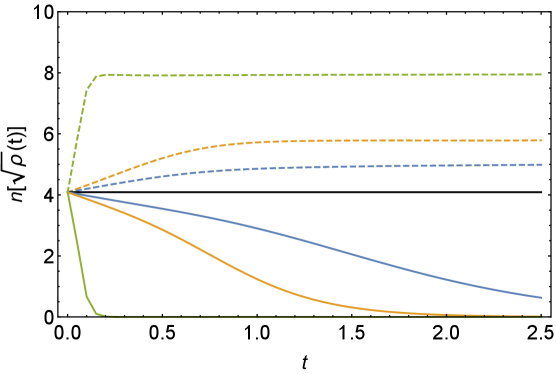
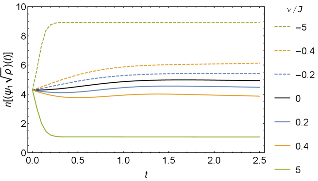
In this appendix, we study the thermal operator growth in Lindbladian SYK model. We consider the initial operators and with . Following the same numerical method in Subsec. 3.1, we construct their time evolution and under the Lindbladian (2) and calculate their sizes and distributions. The size growth and are shown in Fig. 12.
We further define the size difference and the normalized size difference
| (116) | |||
| (117) |
with a normalization factor generalized from Qi:2018quantum , which could be interpreted as the effective operator size of a thermal Majorana fermion under the Lindbladian evolution. We plot both size differences in Fig. 12.
When , decreases to zero at the late times. decreases first and then grows to a plateau lower than at late times. This behavior could be understood as the competition between the dissipation on thermal state and the scrambling of fermion . Such competition is visualized in the size difference , which grows and reaches a plateau. After the normalization, the scale of the thermal fermion size in the right panel of Fig. 12 is similar to the scale of the size of single fermion in Fig. 5, which aligns with the pure SYK result in Qi:2018quantum .
When , both and grow to a finite plateau greater than . The size difference fluctuates at early times and becomes stable at late times. The normalization in fails since can surpass , resulting in a singularity in (117).
Based on the fermion parity, and are nonzero only for even s and odd s respectively. Their size distributions are exhibited in Fig. 14 and Fig. 14.
When , both and tend to concentrate on their lowest possible value after a long evolution. But due to the scrambling of fermion in , it has nonzero distribution at even at late times. Moreover, the distribution in Fig. 14 presents the similar late time behavior with the distribution in Fig 6. When , both and are pushed to the region of large size at late times.
Appendix C Alternative saturated uncertainty relation
By using the Cauchy-Schwarz inequality and the hermicity of , we write the uncertainty relation in another form
| (118) |
The inequality connects the operator size growth to the standard variances of the Liouvillian and the operator size
| (119) |
Comparing the expressions of each term on the two sides (71) (93) (87) in the large limit, we find that the inequality (119) is saturated. Actually, this condition stems from the property of the large solution at finite
| (120) |
References
- (1) E.H. Lieb and D.W. Robinson, The finite group velocity of quantum spin systems, in Statistical Mechanics: Selecta of Elliott H. Lieb, B. Nachtergaele, J.P. Solovej and J. Yngvason, eds., pp. 425–431, Springer Berlin Heidelberg (2004), DOI.
- (2) P. Hayden and J. Preskill, Black holes as mirrors: Quantum information in random subsystems, JHEP 09 (2007) 120 [0708.4025].
- (3) Y. Sekino and L. Susskind, Fast scramblers, JHEP 10 (2008) 065 [0808.2096].
- (4) A.I. Larkin and Y.N. Ovchinnikov, Quasiclassical method in the theory of superconductivity, Sov Phys JETP 28 (1969) 1200.
- (5) S.H. Shenker and D. Stanford, Multiple shocks, JHEP 12 (2014) 046 [1312.3296].
- (6) D.A. Roberts, D. Stanford and L. Susskind, Localized shocks, JHEP 03 (2015) 051 [1409.8180].
- (7) S. Xu and B. Swingle, Scrambling dynamics and out-of-time-ordered correlators in quantum many-body systems, PRX Quantum 5 (2024) 010201.
- (8) D.A. Roberts and B. Swingle, Lieb-Robinson Bound and the Butterfly Effect in Quantum Field Theories, Phys. Rev. Lett. 117 (2016) 091602 [1603.09298].
- (9) S.H. Shenker and D. Stanford, Black holes and the butterfly effect, JHEP 03 (2014) 067 [1306.0622].
- (10) P. Hosur, X.-L. Qi, D.A. Roberts and B. Yoshida, Chaos in quantum channels, JHEP 02 (2016) 004 [1511.04021].
- (11) D.A. Roberts and D. Stanford, Two-dimensional conformal field theory and the butterfly effect, Phys. Rev. Lett. 115 (2015) 131603 [1412.5123].
- (12) D. Stanford, Many-body chaos at weak coupling, JHEP 10 (2016) 009 [1512.07687].
- (13) D.A. Roberts, D. Stanford and A. Streicher, Operator growth in the syk model, JHEP 06 (2018) 122 [1802.02633].
- (14) X.-L. Qi and A. Streicher, Quantum epidemiology: Operator growth, thermal effects, and syk, JHEP 08 (2019) 012 [1810.11958].
- (15) X.-L. Qi, E.J. Davis, A. Periwal and M. Schleier-Smith, Measuring operator size growth in quantum quench experiments, 1906.00524.
- (16) D.E. Parker, X. Cao, A. Avdoshkin, T. Scaffidi and E. Altman, A universal operator growth hypothesis, Phys. Rev. X 9 (2019) 041017 [1812.08657].
- (17) J. Barbón, E. Rabinovici, R. Shir and R. Sinha, On the evolution of operator complexity beyond scrambling, JHEP 10 (2019) 264 [1907.05393].
- (18) A. Avdoshkin and A. Dymarsky, Euclidean operator growth and quantum chaos, Phys. Rev. Res. 2 (2020) 043234 [1911.09672].
- (19) S.-K. Jian, B. Swingle and Z.-Y. Xian, Complexity growth of operators in the syk model and in jt gravity, JHEP 03 (2021) 014 [2008.12274].
- (20) E. Rabinovici, A. Sánchez-Garrido, R. Shir and J. Sonner, Operator complexity: a journey to the edge of krylov space, 2009.01862.
- (21) A. Dymarsky and A. Gorsky, Quantum chaos as delocalization in krylov space, Phys. Rev. B 102 (2020) 085137 [1912.12227].
- (22) M. Carrega, J. Kim and D. Rosa, Unveiling operator growth in syk quench dynamics, 2007.03551.
- (23) A. Kar, L. Lamprou, M. Rozali and J. Sully, Random matrix theory for complexity growth and black hole interiors, JHEP 01 (2022) 016 [2106.02046].
- (24) P. Caputa, J.M. Magan and D. Patramanis, Geometry of krylov complexity, Phys. Rev. Res. 4 (2022) 013041 [2109.03824].
- (25) A. Dymarsky and M. Smolkin, Krylov complexity in conformal field theory, Phys. Rev. D 104 (2021) L081702 [2104.09514].
- (26) E. Rabinovici, A. Sánchez-Garrido, R. Shir and J. Sonner, Krylov localization and suppression of complexity, JHEP 03 (2022) 211 [2112.12128].
- (27) W. Mück and Y. Yang, Krylov complexity and orthogonal polynomials, Nucl. Phys. B 984 (2022) 115948 [2205.12815].
- (28) E. Rabinovici, A. Sánchez-Garrido, R. Shir and J. Sonner, Krylov complexity from integrability to chaos, JHEP 07 (2022) 151 [2207.07701].
- (29) B. Bhattacharjee, X. Cao, P. Nandy and T. Pathak, Krylov complexity in saddle-dominated scrambling, JHEP 05 (2022) 174 [2203.03534].
- (30) B. Bhattacharjee, P. Nandy and T. Pathak, Krylov complexity in large q and double-scaled SYK model, JHEP 08 (2023) 099 [2210.02474].
- (31) A. Avdoshkin, A. Dymarsky and M. Smolkin, Krylov complexity in quantum field theory, and beyond, 2212.14429.
- (32) M. Alishahiha and S. Banerjee, A universal approach to Krylov state and operator complexities, SciPost Phys. 15 (2023) 080 [2212.10583].
- (33) K.-B. Huh, H.-S. Jeong and J.F. Pedraza, Spread complexity in saddle-dominated scrambling, 2312.12593.
- (34) H. Tang, Operator Krylov complexity in random matrix theory, 2312.17416.
- (35) S.E. Aguilar-Gutierrez and A. Rolph, Krylov complexity is not a measure of distance between states or operators, 2311.04093.
- (36) A. Kundu, V. Malvimat and R. Sinha, State dependence of krylov complexity in cfts, 2303.03426.
- (37) C. Beetar, N. Gupta, S.S. Haque, J. Murugan and H.J.R. Van Zyl, Complexity and Operator Growth for Quantum Systems in Dynamic Equilibrium, 2312.15790.
- (38) A. Bhattacharyya, D. Ghosh and P. Nandi, Operator growth and Krylov complexity in Bose-Hubbard model, JHEP 12 (2023) 112 [2306.05542].
- (39) T.Q. Loc, Lanczos spectrum for random operator growth, 2402.07980.
- (40) V. Malvimat, S. Porey and B. Roy, Krylov Complexity in CFTs with SL deformed Hamiltonians, 2402.15835.
- (41) A. Bhattacharya, P.P. Nath and H. Sahu, Speed limits to the growth of Krylov complexity in open quantum systems, 2403.03584.
- (42) V. Balasubramanian, P. Caputa, J.M. Magan and Q. Wu, Quantum chaos and the complexity of spread of states, Phys. Rev. D 106 (2022) 046007 [2202.06957].
- (43) V. Balasubramanian, J.M. Magan and Q. Wu, Tridiagonalizing random matrices, Phys. Rev. D 107 (2023) 126001 [2208.08452].
- (44) J. Erdmenger, S.-K. Jian and Z.-Y. Xian, Universal chaotic dynamics from Krylov space, JHEP 08 (2023) 176 [2303.12151].
- (45) V. Balasubramanian, J.M. Magan and Q. Wu, Quantum chaos, integrability, and late times in the Krylov basis, 2312.03848.
- (46) H.A. Camargo, V. Jahnke, H.-S. Jeong, K.-Y. Kim and M. Nishida, Spectral and Krylov complexity in billiard systems, Phys. Rev. D 109 (2024) 046017 [2306.11632].
- (47) A. Bhattacharyya, S.S. Haque, G. Jafari, J. Murugan and D. Rapotu, Krylov complexity and spectral form factor for noisy random matrix models, JHEP 10 (2023) 157 [2307.15495].
- (48) P. Caputa, H.-S. Jeong, S. Liu, J.F. Pedraza and L.-C. Qu, Krylov complexity of density matrix operators, 2402.09522.
- (49) A. Kitaev, “A simple model of quantum holography.” http://online.kitp.ucsb.edu/online/entangled15/kitaev/ http://online.kitp.ucsb.edu/online/entangled15/kitaev2/, 2015.
- (50) J. Maldacena and D. Stanford, Remarks on the sachdev-ye-kitaev model, Phys. Rev. D 94 (2016) 106002 [1604.07818].
- (51) H.W. Lin and D. Stanford, A symmetry algebra in double-scaled SYK, SciPost Phys. 15 (2023) 234 [2307.15725].
- (52) D.A. Roberts and B. Yoshida, Chaos and complexity by design, JHEP 04 (2017) 121 [1610.04903].
- (53) J. Cotler, N. Hunter-Jones, J. Liu and B. Yoshida, Chaos, complexity, and random matrices, JHEP 11 (2017) 048 [1706.05400].
- (54) A. Nahum, S. Vijay and J. Haah, Operator spreading in random unitary circuits, Phys. Rev. X 8 (2018) 021014 [1705.08975].
- (55) C. von Keyserlingk, T. Rakovszky, F. Pollmann and S. Sondhi, Operator hydrodynamics, otocs, and entanglement growth in systems without conservation laws, Phys. Rev. X 8 (2018) 021013 [1705.08910].
- (56) S. Xu and B. Swingle, Locality, quantum fluctuations, and scrambling, Phys. Rev. X 9 (2019) 031048 [1805.05376].
- (57) J. Maldacena, D. Stanford and Z. Yang, Conformal symmetry and its breaking in two dimensional nearly anti-de-sitter space, PTEP 2016 (2016) 12C104 [1606.01857].
- (58) Y.D. Lensky, X.-L. Qi and P. Zhang, Size of bulk fermions in the syk model, 2002.01961.
- (59) A. Mousatov, Operator size for holographic field theories, 1911.05089.
- (60) H.W. Lin, J. Maldacena and Y. Zhao, Symmetries near the horizon, JHEP 08 (2019) 049 [1904.12820].
- (61) J. Maldacena, S.H. Shenker and D. Stanford, A bound on chaos, JHEP 08 (2016) 106 [1503.01409].
- (62) R. Fan, P. Zhang, H. Shen and H. Zhai, Out-of-Time-Order Correlation for Many-Body Localization, Sci. Bull. 62 (2017) 707 [1608.01914].
- (63) Y. Chen, H. Zhai and P. Zhang, Tunable Quantum Chaos in the Sachdev-Ye-Kitaev Model Coupled to a Thermal Bath, JHEP 07 (2017) 150 [1705.09818].
- (64) Y.-L. Zhang, Y. Huang and X. Chen, Information scrambling in chaotic systems with dissipation, Phys. Rev. B 99 (2019) 014303 [1802.04492].
- (65) J. Li, R. Fan, H. Wang, B. Ye, B. Zeng, H. Zhai et al., Measuring Out-of-Time-Order Correlators on a Nuclear Magnetic Resonance Quantum Simulator, Phys. Rev. X 7 (2017) 031011 [1609.01246].
- (66) M. Gärttner, J.G. Bohnet, A. Safavi-Naini, M.L. Wall, J.J. Bollinger and A.M. Rey, Measuring out-of-time-order correlations and multiple quantum spectra in a trapped ion quantum magnet, Nature Phys. 13 (2017) 781 [1608.08938].
- (67) C.M. Sánchez, A.K. Chattah, K.X. Wei, L. Buljubasich, P. Cappellaro and H.M. Pastawski, Perturbation independent decay of the loschmidt echo in a many-body system, Phys. Rev. Lett. 124 (2020) 030601.
- (68) C.M. Sánchez, A.K. Chattah and H.M. Pastawski, Emergent decoherence induced by quantum chaos in a many-body system: A loschmidt echo observation through nmr, Phys. Rev. A 105 (2022) 052232.
- (69) F.D. Domínguez, M.C. Rodríguez, R. Kaiser, D. Suter and G.A. Álvarez, Decoherence scaling transition in the dynamics of quantum information scrambling, Phys. Rev. A 104 (2021) 012402.
- (70) F.D. Domínguez and G.A. Álvarez, Dynamics of quantum information scrambling under decoherence effects measured via active spin clusters, Phys. Rev. A 104 (2021) 062406 [2107.03870].
- (71) X. Mi et al., Information scrambling in quantum circuits, Science 374 (2021) abg5029 [2101.08870].
- (72) J. Cotler, T. Schuster and M. Mohseni, Information-theoretic hardness of out-of-time-order correlators, Phys. Rev. A 108 (2023) 062608 [2208.02256].
- (73) B. Swingle, G. Bentsen, M. Schleier-Smith and P. Hayden, Measuring the scrambling of quantum information, Phys. Rev. A 94 (2016) 040302 [1602.06271].
- (74) R. Islam, R. Ma, P.M. Preiss, M.E. Tai, A. Lukin, M. Rispoli et al., Measuring entanglement entropy through the interference of quantum many-body twins, 1509.01160.
- (75) K.A. Landsman, C. Figgatt, T. Schuster, N.M. Linke, B. Yoshida, N.Y. Yao et al., Verified Quantum Information Scrambling, Nature 567 (2019) 61 [1806.02807].
- (76) M.S. Blok, V.V. Ramasesh, T. Schuster, K. O’Brien, J.M. Kreikebaum, D. Dahlen et al., Quantum Information Scrambling on a Superconducting Qutrit Processor, Phys. Rev. X 11 (2021) 021010 [2003.03307].
- (77) T. Brydges, A. Elben, P. Jurcevic, B. Vermersch, C. Maier, B.P. Lanyon et al., Probing rényi entanglement entropy via randomized measurements, Science 364 (2019) 260.
- (78) M.K. Joshi, A. Elben, B. Vermersch, T. Brydges, C. Maier, P. Zoller et al., Quantum information scrambling in a trapped-ion quantum simulator with tunable range interactions, Phys. Rev. Lett. 124 (2020) 240505.
- (79) P.D. Blocher, K. Chinni, S. Omanakuttan and P.M. Poggi, Probing scrambling and operator size distributions using random mixed states and local measurements, 2305.16992.
- (80) H.-P. Breuer and F. Petruccione, The theory of open quantum systems, Oxford University Press, USA (2002).
- (81) D.A. Lidar, Lecture notes on the theory of open quantum systems, arXiv preprint arXiv:1902.00967 (2019) .
- (82) D. Manzano, A short introduction to the lindblad master equation, Aip Advances 10 (2020) .
- (83) S. Denisov, T. Laptyeva, W. Tarnowski, D. Chruściński and K. Życzkowski, Universal spectra of random Lindblad operators, Phys. Rev. Lett. 123 (2019) 140403 [1811.12282].
- (84) T. Schuster and N.Y. Yao, Operator Growth in Open Quantum Systems, Phys. Rev. Lett. 131 (2023) 160402 [2208.12272].
- (85) A. Kulkarni, T. Numasawa and S. Ryu, Lindbladian dynamics of the Sachdev-Ye-Kitaev model, Phys. Rev. B 106 (2022) 075138 [2112.13489].
- (86) K. Kawabata, A. Kulkarni, J. Li, T. Numasawa and S. Ryu, Dynamical quantum phase transitions in Sachdev-Ye-Kitaev Lindbladians, Phys. Rev. B 108 (2023) 075110 [2210.04093].
- (87) A.M. García-García, L. Sá, J.J.M. Verbaarschot and J.P. Zheng, Keldysh wormholes and anomalous relaxation in the dissipative Sachdev-Ye-Kitaev model, Phys. Rev. D 107 (2023) 106006 [2210.01695].
- (88) L. Sá, P. Ribeiro and T. Prosen, Lindbladian dissipation of strongly-correlated quantum matter, Phys. Rev. Res. 4 (2022) L022068 [2112.12109].
- (89) B. Bhattacharjee, P. Nandy and T. Pathak, Operator dynamics in Lindbladian SYK: a Krylov complexity perspective, JHEP 01 (2024) 094 [2311.00753].
- (90) C. Liu, H. Tang and H. Zhai, Krylov complexity in open quantum systems, 2207.13603.
- (91) B. Bhattacharjee, X. Cao, P. Nandy and T. Pathak, Operator growth in open quantum systems: lessons from the dissipative syk, 2212.06180.
- (92) A. Bhattacharya, P. Nandy, P.P. Nath and H. Sahu, Operator growth and krylov construction in dissipative open quantum systems, JHEP 12 (2022) 081 [2207.05347].
- (93) A. Bhattacharya, P. Nandy, P.P. Nath and H. Sahu, On krylov complexity in open systems: an approach via bi-lanczos algorithm, 2303.04175.
- (94) A. Bhattacharya, R.N. Das, B. Dey and J. Erdmenger, Spread complexity for measurement-induced non-unitary dynamics and Zeno effect, 2312.11635.
- (95) P. Zhang and Z. Yu, Dynamical transition of operator size growth in quantum systems embedded in an environment, Phys. Rev. Lett. 130 (2023) 250401.
- (96) P. Gao, D.L. Jafferis and A.C. Wall, Traversable Wormholes via a Double Trace Deformation, JHEP 12 (2017) 151 [1608.05687].
- (97) J. Maldacena and X.-L. Qi, Eternal traversable wormhole, arXiv:1804.00491 (2018) .
- (98) A. Milekhin and F.K. Popov, Measurement-induced phase transition in teleportation and wormholes, 2210.03083.
- (99) T. Prosen, PT-Symmetric Quantum Liouvillean Dynamics, Phys. Rev. Lett. 109 (2012) 090404 [1207.4395].
- (100) A.M. García-García, L. Sá, J.J.M. Verbaarschot and C. Yin, Towards a classification of PT-symmetric quantum systems: from dissipative dynamics to topology and wormholes, 2311.15677.
- (101) C.M. Bender and S. Boettcher, Real spectra in non-hermitian hamiltonians having symmetry, Phys. Rev. Lett. 80 (1998) 5243.
- (102) A. Mostafazadeh, Pseudo-Hermiticity versus PT symmetry: The necessary condition for the reality of the spectrum, J. Math. Phys. 43 (2002) 205.
- (103) A. Mostafazadeh, PseudoHermiticity versus PT symmetry 2. A Complete characterization of nonHermitian Hamiltonians with a real spectrum, J. Math. Phys. 43 (2002) 2814.
- (104) A. Mostafazadeh, PseudoHermiticity versus PT symmetry 3: Equivalence of pseudoHermiticity and the presence of antilinear symmetries, J. Math. Phys. 43 (2002) 3944.
- (105) R. Zhang, H. Qin and J. Xiao, PT-symmetry entails pseudo-Hermiticity regardless of diagonalizability, J. Math. Phys. 61 (2020) 012101.
- (106) J.S. Cotler, G. Gur-Ari, M. Hanada, J. Polchinski, P. Saad, S.H. Shenker et al., Black holes and random matrices, JHEP 05 (2017) 118 [1611.04650].
- (107) Y.-N. Zhou, L. Mao and H. Zhai, Rényi entropy dynamics and Lindblad spectrum for open quantum systems, Phys. Rev. Res. 3 (2021) 043060 [2101.11236].
- (108) A.M. García-García and J.J.M. Verbaarschot, Spectral and thermodynamic properties of the sachdev-ye-kitaev model, Phys. Rev. D 94 (2016) 126010 [1610.03816].
- (109) Y.-Z. You, A.W. Ludwig and C. Xu, Sachdev-ye-kitaev model and thermalization on the boundary of many-body localized fermionic symmetry-protected topological states, Physical Review B 95 (2017) 115150.
- (110) D.C. Brody, Biorthogonal quantum mechanics, J. Phys. A 47 (2013) 035305.
- (111) A. Streicher, SYK Correlators for All Energies, JHEP 02 (2020) 048 [1911.10171].
- (112) P. Gao and D.L. Jafferis, A traversable wormhole teleportation protocol in the SYK model, JHEP 07 (2021) 097 [1911.07416].
- (113) B. Yan, L. Cincio and W.H. Zurek, Information Scrambling and Loschmidt Echo, Phys. Rev. Lett. 124 (2020) 160603 [1903.02651].
- (114) T. Gorin, T. Prosen, T.H. Seligman and M. Žnidarič, Dynamics of loschmidt echoes and fidelity decay, Physics Reports 435 (2006) 33.
- (115) A. Goussev, R.A. Jalabert, H.M. Pastawski and D. Wisniacki, Loschmidt echo, arXiv preprint arXiv:1206.6348 (2012) .
- (116) R.A. Jalabert and H.M. Pastawski, Environment-independent decoherence rate in classically chaotic systems, Phys. Rev. Lett. 86 (2001) 2490.
- (117) Y. Gu, X.-L. Qi and D. Stanford, Local criticality, diffusion and chaos in generalized sachdev-ye-kitaev models, JHEP 05 (2017) 125 [1609.07832].
- (118) Y. Gu and A. Kitaev, On the relation between the magnitude and exponent of OTOCs, JHEP 02 (2019) 075 [1812.00120].
- (119) Y. Gu, A. Kitaev and P. Zhang, A two-way approach to out-of-time-order correlators, JHEP 03 (2022) 133 [2111.12007].
- (120) A.M. García-García, J.J.M. Verbaarschot and J.-p. Zheng, The Lyapunov exponent as a signature of dissipative many-body quantum chaos, 2403.12359.
- (121) N. Hörnedal, N. Carabba, A.S. Matsoukas-Roubeas and A. del Campo, Ultimate speed limits to the growth of operator complexity, Commun. Phys. 5 (2022) 207 [2202.05006].
- (122) S.-K. Jian, Z.-Y. Xian and H. Yao, Quantum criticality and duality in the Sachdev-Ye-Kitaev/AdS2 chain, Phys. Rev. B 97 (2018) 205141 [1709.02810].
- (123) H.W. Lin, The bulk hilbert space of double scaled syk, JHEP 11 (2022) 060 [2208.07032].
- (124) J.M. Maldacena, Eternal black holes in anti-de sitter, JHEP 04 (2003) 021 [hep-th/0106112].
- (125) Z.-Y. Xian and L. Zhao, Wormholes and the Thermodynamic Arrow of Time, Phys. Rev. Res. 2 (2020) 043095 [1911.03021].
- (126) S. He and Z.-Y. Xian, TT¯ deformation on multiquantum mechanics and regenesis, Phys. Rev. D 106 (2022) 046002 [2104.03852].
- (127) D. Areán, K. Landsteiner and I. Salazar Landea, Non-hermitian holography, SciPost Phys. 9 (2020) 032 [1912.06647].
- (128) Z.-Y. Xian, D. Rodríguez Fernández, Z. Chen, Y. Liu and R. Meyer, Electric conductivity in non-Hermitian holography, SciPost Phys. 16 (2024) 004 [2304.11183].
- (129) Y. Chen, V. Ivo and J. Maldacena, Comments on the double cone wormhole, 2310.11617.