Ophiuchus: Scalable Modeling of Protein Structures through Hierarchical Coarse-graining SO(3)-Equivariant Autoencoders
Abstract
Three-dimensional native states of natural proteins display recurring and hierarchical patterns. Yet, traditional graph-based modeling of protein structures is often limited to operate within a single fine-grained resolution, and lacks hourglass neural architectures to learn those high-level building blocks. We narrow this gap by introducing Ophiuchus, an SO(3)-equivariant coarse-graining model that efficiently operates on all-atom protein structures. Our model departs from current approaches that employ graph modeling, instead focusing on local convolutional coarsening to model sequence-motif interactions with efficient time complexity in protein length. We measure the reconstruction capabilities of Ophiuchus across different compression rates, and compare it to existing models. We examine the learned latent space and demonstrate its utility through conformational interpolation. Finally, we leverage denoising diffusion probabilistic models (DDPM) in the latent space to efficiently sample protein structures. Our experiments demonstrate Ophiuchus to be a scalable basis for efficient protein modeling and generation.
1 Introduction
Proteins form the basis of all biological processes and understanding them is critical to biological discovery, medical research and drug development. Their three-dimensional structures often display modular organization across multiple scales, making them promising candidates for modeling in motif-based design spaces [Bystroff & Baker (1998); Mackenzie & Grigoryan (2017); Swanson et al. (2022)]. Harnessing these coarser, lower-frequency building blocks is of great relevance to the investigation of the mechanisms behind protein evolution, folding and dynamics [Mackenzie et al. (2016)], and may be instrumental in enabling more efficient computation on protein structural data through coarse and latent variable modeling [Kmiecik et al. (2016); Ramaswamy et al. (2021)].
Recent developments in deep learning architectures applied to protein sequences and structures demonstrate the remarkable capabilities of neural models in the domain of protein modeling and design [Jumper et al. (2021); Baek et al. (2021b); Ingraham et al. (2022); Watson et al. (2022)]. Still, current state-of-the-art architectures lack the structure and mechanisms to directly learn and operate on modular protein blocks.
To fill this gap, we introduce Ophiuchus, a deep SO(3)-equivariant model that captures joint encodings of sequence-structure motifs of all-atom protein structures. Our model is a novel autoencoder that uses one-dimensional sequence convolutions on geometric features to learn coarsened representations of proteins. Ophiuchus outperforms existing SO(3)-equivariant autoencoders [Fu et al. (2023)] on the protein reconstruction task. We present extensive ablations of model performance across different autoencoder layouts and compression settings. We demonstrate that our model learns a robust and structured representation of protein structures by learning a denoising diffusion probabilistic model (DDPM) [Ho et al. (2020)] in the latent space. We find Ophiuchus to enable significantly faster sampling of protein structures, as compared to existing diffusion models [Wu et al. (2022a); Yim et al. (2023); Watson et al. (2023)], while producing unconditional samples of comparable quality and diversity.
Our main contributions are summarized as follows:
-
•
Novel Autoencoder: We introduce a novel SO(3)-equivariant autoencoder for protein sequence and all-atom structure representation. We propose novel learning algorithms for coarsening and refining protein representations, leveraging irreducible representations of SO(3) to efficiently model geometric information. We demonstrate the power of our latent space through unsupervised clustering and latent interpolation.
-
•
Extensive Ablation: We offer an in-depth examination of our architecture through extensive ablation across different protein lengths, coarsening resolutions and model sizes. We study the trade-off of producing a coarsened representation of a protein at different resolutions and the recoverability of its sequence and structure.
-
•
Latent Diffusion: We explore a novel generative approach to proteins by performing latent diffusion on geometric feature representations. We train diffusion models for multiple resolutions, and provide diverse benchmarks to assess sample quality. To the best of our knowledge, this is the first generative model to directly produce all-atom structures of proteins.
2 Background and Related Work
2.1 Modularity and Hierarchy in Proteins
Protein sequences and structures display significant degrees of modularity. [Vallat et al. (2015)] introduces a library of common super-secondary structural motifs (Smotifs), while [Mackenzie et al. (2016)] shows protein structural space to be efficiently describable by small tertiary alphabets (TERMs). Motif-based methods have been successfully used in protein folding and design [Bystroff & Baker (1998); Li et al. (2022)]. Inspired by this hierarchical nature of proteins, our proposed model learns coarse-grained representations of protein structures.
2.2 Symmetries in Neural Architecture for Biomolecules
Learning algorithms greatly benefit from proactively exploiting symmetry structures present in their data domain [Bronstein et al. (2021); Smidt (2021)]. In this work, we investigate three relevant symmetries for the domain of protein structures:
Euclidean Equivariance of Coordinates and Feature Representations. Neural models equipped with roto-translational (Euclidean) invariance or equivariance have been shown to outperform competitors in molecular and point cloud tasks [Townshend et al. (2022); Miller et al. (2020); Deng et al. (2021)]. Similar results have been extensively reported across different structural tasks of protein modeling [Liu et al. (2022); Jing et al. (2021)]. Our proposed model takes advantage of Euclidean equivariance both in processing of coordinates and in its internal feature representations, which are composed of scalars and higher order geometric tensors [Thomas et al. (2018); Weiler et al. (2018)].
Translation Equivariance of Sequence. One-dimensional Convolutional Neural Networks (CNNs) have been demonstrated to successfully model protein sequences across a variety of tasks [Karydis (2017); Hou et al. (2018); Lee et al. (2019); Yang et al. (2022)]. These models capture sequence-motif representations that are equivariant to translation of the sequence. However, sequential convolution is less common in architectures for protein structures, which are often cast as Graph Neural Networks (GNNs) [Zhang et al. (2021)]. Notably, [Fan et al. (2022)] proposes a CNN network to model the regularity of one-dimensional sequences along with three-dimensional structures, but they restrict their layout to coarsening. In this work, we further integrate geometry into sequence by directly using three-dimensional vector feature representations and transformations in 1D convolutions. We use this CNN to investigate an autoencoding approach to protein structures.
Permutation Invariances of Atomic Order. In order to capture the permutable ordering of atoms, neural models of molecules are often implemented with permutation-invariant GNNs [Wieder et al. (2020)]. Nevertheless, protein structures are sequentially ordered, and most standard side-chain heavy atoms are readily orderable, with exception of four residues [Jumper et al. (2021)]. We use this fact to design an efficient approach to directly model all-atom protein structures, introducing a method to parse atomic positions in parallel channels as roto-translational equivariant feature representations.
2.3 Unsupervised Learning of Proteins
Unsupervised techniques for capturing protein sequence and structure have witnessed remarkable advancements in recent years [Lin et al. (2023); Elnaggar et al. (2023); Zhang et al. (2022)]. Amongst unsupervised methods, autoencoder models learn to produce efficient low-dimensional representations using an informational bottleneck. These models have been successfully deployed to diverse protein tasks of modeling and sampling [Eguchi et al. (2020); Lin et al. (2021); Wang et al. (2022); Mansoor et al. (2023); Visani et al. (2023)], and have received renewed attention for enabling the learning of coarse representations of molecules [Wang & Gómez-Bombarelli (2019); Yang & Gómez-Bombarelli (2023); Winter et al. (2021); Wehmeyer & Noé (2018); Ramaswamy et al. (2021)]. However, existing three-dimensional autoencoders for proteins do not have the structure or mechanisms to explore the extent to which coarsening is possible in proteins. In this work, we fill this gap with extensive experiments on an autoencoder for deep protein representation coarsening.
2.4 Denoising Diffusion for Proteins
Denoising Diffusion Probabilistic Models (DDPM) [Sohl-Dickstein et al. (2015); Ho et al. (2020)] have found widespread adoption through diverse architectures for generative sampling of protein structures. Chroma [Ingraham et al. (2022)] trains random graph message passing through roto-translational invariant features, while RFDiffusion [Watson et al. (2022)] fine-tunes pretrained folding model RoseTTAFold [Baek et al. (2021a)] to denoising, employing SE(3)-equivariant transformers in structural decoding [Fuchs et al. (2020)]. [Yim et al. (2023); Anand & Achim (2022)] generalize denoising diffusion to frames of reference, employing Invariant Point Attention [Jumper et al. (2021)] to model three dimensions, while FoldingDiff [Wu et al. (2022a)] explores denoising in angular space. More recently, [Fu et al. (2023)] proposes a latent diffusion model on coarsened representations learned through Equivariant Graph Neural Networks (EGNN) [Satorras et al. (2022)]. In contrast, our model uses roto-translation equivariant features to produce increasingly richer structural representations from autoencoded sequence and coordinates. We propose a novel latent diffusion model that samples directly in this space for generating protein structures.
3 The Ophiuchus Architecture
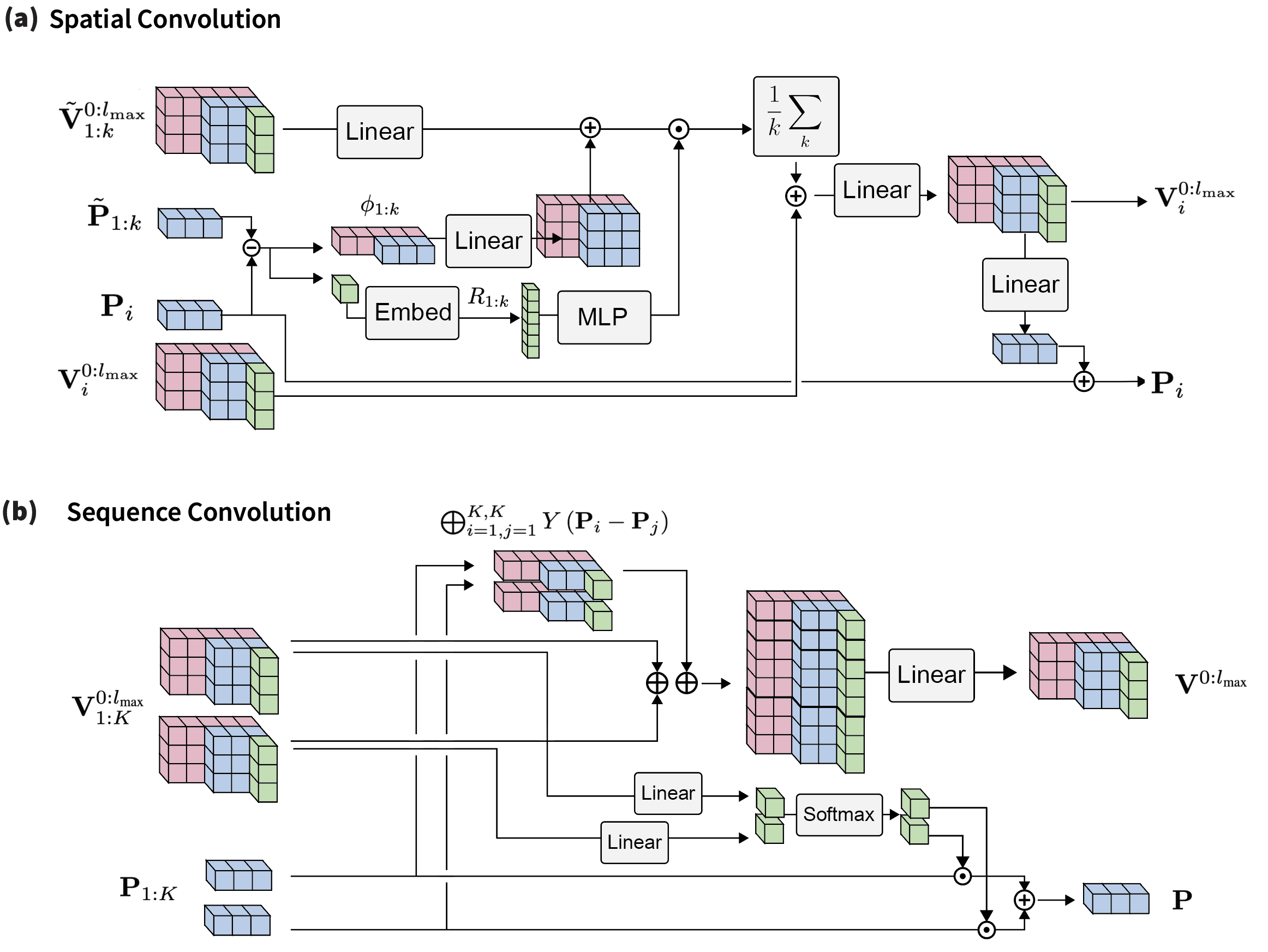
We represent a protein as a sequence of residues each with an anchor position and a tensor of irreducible representations of SO(3) , where and degree . A residue state is defined as . These representations are directly produced from sequence labels and all-atom positions, as we describe in the Atom Encoder/Decoder sections. To capture the diverse interactions within a protein, we propose three main components. Self-Interaction learns geometric representations of each residue independently, modeling local interactions of atoms within a single residue. Sequence Convolution simultaneously updates sequential segments of residues, modeling inter-residue interactions between sequence neighbors. Finally, Spatial Convolution employs message-passing of geometric features to model interactions of residues that are nearby in 3D space. We compose these three modules to build an hourglass architecture.
3.1 All-Atom Atom Encoder and Decoder
Given a particular -th residue, let denote its residue label, denote the global position of its alpha carbon (), and the position of all other atoms relative to . We produce initial residue representations by setting anchors , scalars , and geometric vectors to explicitly encode relative atomic positions .
In particular, provided the residue label , the heavy atoms of most standard protein residues are readily put in a canonical order, enabling direct treatment of atom positions as a stack of signals on SO(3): . However, some of the standard residues present two-permutations within their atom configurations, in which pairs of atoms have ordering indices (, ) that may be exchanged (Appendix A.1). To handle these cases, we instead use geometric vectors to encode the center and the unsigned difference between the positions of the pair, where is a spherical harmonics projector of degree . This signal is invariant to corresponding atomic two-flips, while still directly carrying information about positioning and angularity. To invert this encoding, we invert a signal of degree into two arbitrarily ordered vectors of degrees . Please refer to Appendix A.2 for further details.
This processing makes Ophiuchus strictly blind to ordering flips of permutable atoms, while still enabling it to operate directly on all atoms in an efficient, stacked representation. In Appendix A.1, we illustrate how this approach correctly handles the geometry of side-chain atoms.
3.2 Self-Interaction
Our Self-Interaction is designed to model the internal interactions of atoms within each residue. This transformation updates the feature vectors centered at the same residue . Importantly, it blends feature vectors of varying degrees by employing tensor products of the features with themselves. We offer two implementations of these tensor products to cater to different computational needs. Our Self-Interaction module draws inspiration from MACE [Batatia et al. (2022)]. For a comprehensive explanation, please refer to Appendix A.3.
3.3 Sequence Convolution
To take advantage of the sequential nature of proteins, we propose a one-dimensional, roto-translational equivariant convolutional layer for acting on geometric features and positions of sequence neighbors. Given a kernel window size and stride , we concatenate representations with the same value. Additionally, we include normalized relative vectors between anchoring positions . Following conventional CNN architectures, this concatenated representation undergoes a linear transformation. The scalars in the resulting representation are then converted into weights, which are used to combine window coordinates into a new coordinate. To ensure translational equivariance, these weights are constrained to sum to one.
When , sequence convolutions reduce the dimensionality along the sequence axis, yielding mixed representations and coarse coordinates. To reverse this procedure, we introduce a transpose convolution algorithm that uses its features to spawn coordinates. For further details, please refer to Appendix A.6.
3.4 Spatial Convolution
To capture interactions of residues that are close in three-dimensional space, we introduce the Spatial Convolution. This operation updates representations and positions through message passing within k-nearest spatial neighbors. Message representations incorporate SO(3) signals from the vector difference between neighbor coordinates, and we aggregate messages with a permutation-invariant means. After aggregation, we linearly transform the vector representations into a an update for the coordinates.
3.5 Deep Coarsening Autoencoder
We compose Space Convolution, Self-Interaction and Sequence Convolution modules to define a coarsening/refining block. The block mixes representations across all relevant axes of the domain while producing coarsened, downsampled positions and mixed embeddings. The reverse result – finer positions and decoupled embeddings – is achieved by changing the standard Sequence Convolution to its transpose counterpart. When employing sequence convolutions of stride , we increase the dimensionality of the feature representation according to a rescaling factor hyperparameter . We stack coarsening blocks to build a deep neural encoder (Alg.7), and symetrically refining blocks to build a decoder (Alg. 8).
3.6 Autoencoder Reconstruction Losses
We use a number of reconstruction losses to ensure good quality of produced proteins.
Vector Map Loss. We train the model by directly comparing internal three-dimensional vector difference maps. Let denote the internal vector map between all atoms in our data, that is, . We define the vector map loss as [Huber (1992)]. When computing this loss, an additional stage is employed for processing permutation symmetry breaks. More details can be found in Appendix B.1.
Residue Label Cross Entropy Loss. We train the model to predict logits over alphabet for each residue. We use the cross entropy between predicted logits and ground labels:
Chemistry Losses. We incorporate norm-based losses for comparing bonds, angles and dihedrals between prediction and ground truth. For non-bonded atoms, a clash loss is evaluated using standard Van der Waals atomic radii (Appendix B.2)
Please refer to Appendix B for further details on the loss.
3.7 Latent Diffusion
We train an SO(3)-equivariant DDPM [Ho et al. (2020); Sohl-Dickstein et al. (2015)] on the latent space of our autoencoder. We pre-train an autoencoder and transform each protein from the dataset into a geometric tensor of irreducible representations of SO(3): . We attach a diffusion process of steps on the latent variables, making and . We follow the parameterization described in [Salimans & Ho (2022)], and train a denoising model to reconstruct the original data from its noised version :
In order to ensure that bottleneck representations are well-behaved for generation purposes, we regularize the latent space of our autoencoder (Appendix B.3). We build a denoising network with layers of Self-Interaction. Please refer to Appendix F for further details.
3.8 Implementation
4 Methods and Results
4.1 Autoencoder Architecture Comparison
We compare Ophiuchus to the architecture proposed in [Fu et al. (2023)], which uses the EGNN-based architecture [Satorras et al. (2022)] for autoencoding protein backbones. To the best of our knowledge, this is the only other model that attempts protein reconstruction in three-dimensions with roto-translation equivariant networks. For demonstration purposes, we curate a small dataset of protein -backbones from the PDB with lengths between 16 and 64 and maximum resolution of up to 1.5 Å, resulting in 1267 proteins. We split the data into train, validation and test sets with ratio [0.8, 0.1, 0.1]. In table 1, we report the test performance at best validation step, while avoiding over-fitting during training.
Model Downsampling Factor Channels/Layer Params [1e6] C-RMSD (Å) Residue Acc. () EGNN 2 [32, 32] 0.68 1.01 88 EGNN 4 [32, 32, 48] 1.54 1.12 80 EGNN 8 [32, 32, 48, 72] 3.30 2.06 73 EGNN 16 [32, 32, 48, 72, 108] 6.99 11.4 25 Ophiuchus 2 [5, 7] 0.018 0.11 98 Ophiuchus 4 [5, 7, 10] 0.026 0.14 97 Ophiuchus 8 [5, 7, 10, 15] 0.049 0.36 79 Ophiuchus 16 [5, 7, 10, 15, 22] 0.068 0.43 37
We find that Ophiuchus vastly outperforms the EGNN-based architecture. Ophiuchus recovers the protein sequence and backbone with significantly better accuracy, while using orders of magnitude less parameters. Refer to Appendix C for further details.
4.2 Architecture Ablation
To investigate the effects of different architecture layouts and coarsening rates, we train different instantiations of Ophiuchus to coarsen representations of contiguous 160-sized protein fragments from the Protein Databank (PDB) [Berman et al. (2000)]. We filter out entries tagged with resolution higher than 2.5 Å, and total sequence lengths larger than 512. We also ensure proteins in the dataset have same chirality. For ablations, the sequence convolution uses kernel size of 5 and stride 3, channel rescale factor per layer is one of {1.5, 1.7, 2.0}, and the number of downsampling layers ranges in 3-5. The initial residue representation uses 16 channels, where each channel is composed of one scalar () and one 3D vector (). All experiments were repeated 3 times with different initialization seeds and data shuffles.
Downsampling Factor Channels/Layer # Params [1e6] C-RMSD (Å) All-Atom RMSD (Å) GDT-TS GDT-HA Residue Acc. (%) 17 [16, 24, 36] 0.34 0.90 0.20 0.68 0.08 94 3 76 4 97 2 17 [16, 27, 45] 0.38 0.89 0.21 0.70 0.09 94 3 77 5 98 1 17 [16, 32, 64] 0.49 1.02 0.25 0.72 0.09 92 4 73 5 98 1 53 [16, 24, 36, 54] 0.49 1.03 0.18 0.83 0.10 91 3 72 5 60 4 53 [16, 27, 45, 76] 0.67 0.92 0.19 0.77 0.09 93 3 75 5 66 4 53 [16, 32, 64, 128] 1.26 1.25 0.32 0.80 0.16 86 5 65 6 67 5 160 [16, 24, 36, 54, 81] 0.77 1.67 0.24 1.81 0.16 77 4 54 5 17 3 160 [16, 27, 45, 76, 129] 1.34 1.39 0.23 1.51 0.17 83 4 60 5 17 3 160 [16, 32, 64, 128, 256] 3.77 1.21 0.25 1.03 0.15 87 5 65 6 27 4
In our experiments we find a trade-off between domain coarsening factor and reconstruction performance. In Table 2 we show that although residue recovery suffers from large downsampling factors, structure recovery rates remain comparable between various settings. Moreover, we find that we are able to model all atoms in proteins, as opposed to only C atoms (as commonly done), and still recover the structure with high precision. These results demonstrate that protein data can be captured effectively and efficiently using sequence-modular geometric representations. We directly utilize the learned compact latent space as shown below by various examples. For further ablation analysis please refer to Appendix D.
4.3 Latent Conformational Interpolation
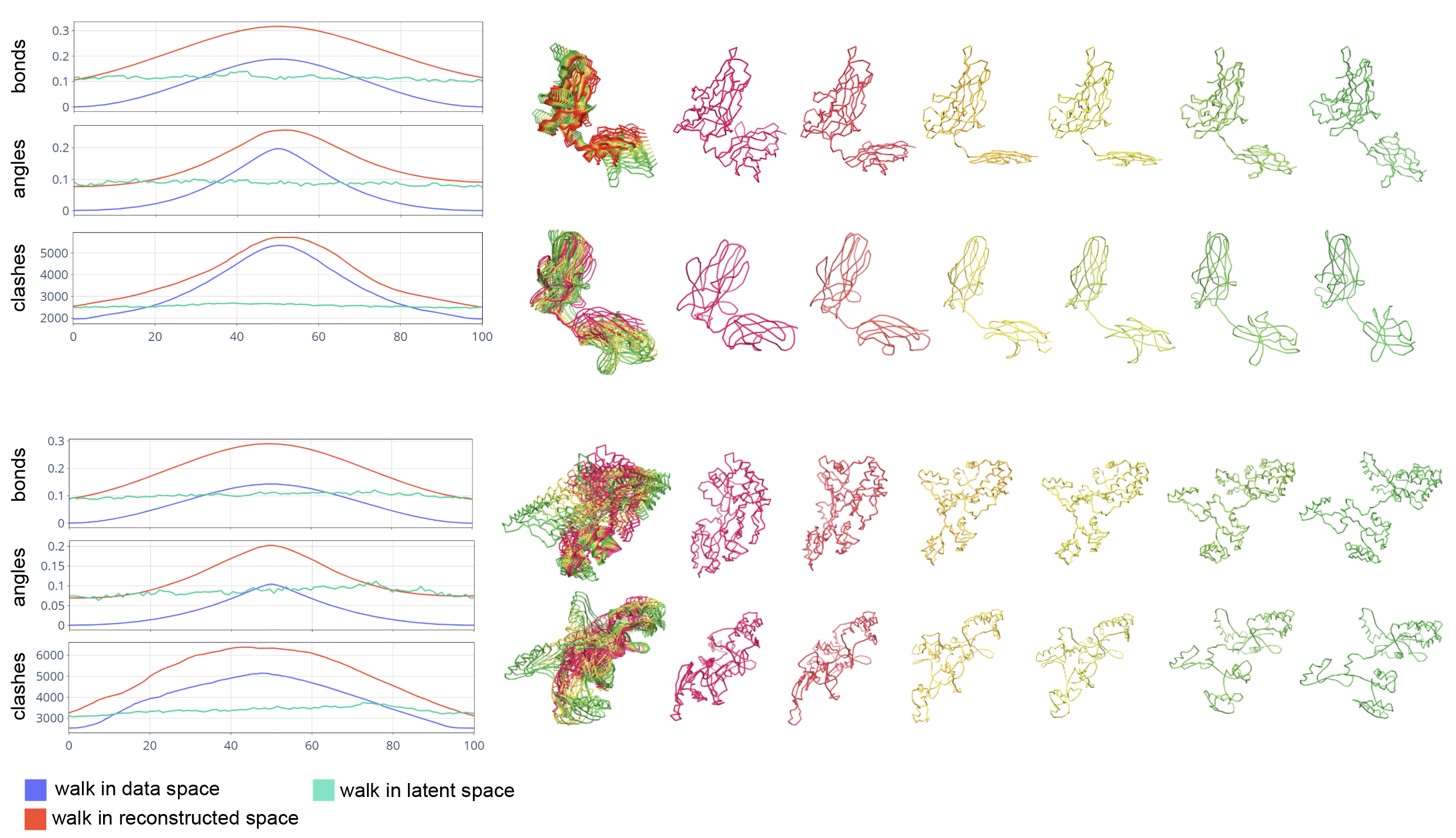
To demonstrate the power of Ophiuchus’s geometric latent space, we show smooth interpolation between two states of a protein structure without explicit latent regularization (as opposed to [Ramaswamy et al. (2021)]). We use the PDBFlex dataset [Hrabe et al. (2016)] and pick pairs of flexible proteins. Conformational snapshots of these proteins are used as the endpoints for the interpolation. We train a large Ophiuchus reconstruction model on general PDB data. The model coarsens up to 485-residue proteins into a single high-order geometric representation using 6 convolutional downsampling layers each with kernel size 5 and stride 3. The endpoint structures are compressed into single geometric representation which enables direct latent interpolation in feature .
We compare the results of linear interpolation in the latent space against linear interpolation in the coordinate domain (Fig. 11). To determine chemical validity of intermediate states, we scan protein data to quantify average bond lengths and inter-bond angles. We calculate the deviation from these averages for bonds and angles of interpolated structures. Additionally, we measure atomic clashes by counting collisions of Van der-Waals radii of non-bonded atoms (Fig. 11). Although the latent and autoencoder-reconstructed interpolations perform worse than direct interpolation near the original data points, we find that only the latent interpolation structures maintain a consistent profile of chemical validity throughout the trajectory, while direct interpolation in the coordinate domain disrupts it significantly. This demonstrates that the learned latent space compactly and smoothly represents protein conformations.
4.4 Latent Diffusion Experiments and Benchmarks
Our ablation study (Tables 2 and 4) shows successful recovery of backbone structure of large proteins even for large coarsening rates. However, we find that for sequence reconstruction, larger models and longer training times are required. During inference, all-atom models rely on the decoding of the sequence, thus making significantly harder for models to resolve all-atom generation. Due to computational constraints, we investigate all-atom latent diffusion models for short sequence lengths, and focus on backbone models for large proteins. We train the all-atom models with mini-proteins of sequences shorter than 64 residues, leveraging the MiniProtein scaffolds dataset produced by [Cao et al. (2022)]. In this regime, our model is precise and successfully reconstructs sequence and all-atom positions. We also instantiate an Ophiuchus model for generating the backbone trace for large proteins of length 485. For that, we train our model on the PDB data curated by [Yim et al. (2023)]. We compare the quality of diffusion samples from our model to RFDiffusion (T=50) and FrameDiff (N=500 and noise=0.1) samples of similar lengths. We generated 500 unconditional samples from each of the models for evaluation.
In Table 3 we compare sampling the latent space of Ophiuchus to existing models. We find that our model performs comparably in terms of different generated sample metrics, while enabling orders of magnitude faster sampling for proteins. For all comparisons we run all models on a single RTX6000 GPU. Please refer to Appendix F for more details.
5 Conclusion and Future Work
In this work, we introduced a new autoencoder model for protein structure and sequence representation. Through extensive ablation on its architecture, we quantified the trade-offs between model complexity and representation quality. We demonstrated the power of our learned representations in latent interpolation, and investigated its usage as basis for efficient latent generation of backbone and all-atom protein structures. Our studies suggest Ophiuchus to provide a strong foundation for constructing state-of-the-art protein neural architectures. In future work, we will investigate scaling Ophiuchus representations and generation to larger proteins and additional molecular domains.
References
- Anand & Achim (2022) Namrata Anand and Tudor Achim. Protein structure and sequence generation with equivariant denoising diffusion probabilistic models, 2022.
- Ba et al. (2016) Jimmy Lei Ba, Jamie Ryan Kiros, and Geoffrey E. Hinton. Layer normalization, 2016.
- Baek et al. (2021a) Minkyung Baek, Frank DiMaio, Ivan Anishchenko, Justas Dauparas, Sergey Ovchinnikov, Gyu Rie Lee, Jue Wang, Qian Cong, Lisa N. Kinch, R. Dustin Schaeffer, Claudia Millán, Hahnbeom Park, Carson Adams, Caleb R. Glassman, Andy DeGiovanni, Jose H. Pereira, Andria V. Rodrigues, Alberdina A. van Dijk, Ana C. Ebrecht, Diederik J. Opperman, Theo Sagmeister, Christoph Buhlheller, Tea Pavkov-Keller, Manoj K. Rathinaswamy, Udit Dalwadi, Calvin K. Yip, John E. Burke, K. Christopher Garcia, Nick V. Grishin, Paul D. Adams, Randy J. Read, and David Baker. Accurate prediction of protein structures and interactions using a three-track neural network. Science, 373(6557):871–876, August 2021a. doi: 10.1126/science.abj8754. URL https://doi.org/10.1126/science.abj8754.
- Baek et al. (2021b) Minkyung Baek, Frank DiMaio, Ivan Anishchenko, Justas Dauparas, Sergey Ovchinnikov, Gyu Rie Lee, Jue Wang, Qian Cong, Lisa N Kinch, R Dustin Schaeffer, et al. Accurate prediction of protein structures and interactions using a three-track neural network. Science, 373(6557):871–876, 2021b.
- Batatia et al. (2022) Ilyes Batatia, David Peter Kovacs, Gregor N. C. Simm, Christoph Ortner, and Gabor Csanyi. MACE: Higher order equivariant message passing neural networks for fast and accurate force fields. In Alice H. Oh, Alekh Agarwal, Danielle Belgrave, and Kyunghyun Cho (eds.), Advances in Neural Information Processing Systems, 2022. URL https://openreview.net/forum?id=YPpSngE-ZU.
- Bentley (1975) Jon Louis Bentley. Multidimensional binary search trees used for associative searching. Communications of the ACM, 18(9):509–517, 1975.
- Berman et al. (2000) Helen M Berman, John Westbrook, Zukang Feng, Gary Gilliland, Talapady N Bhat, Helge Weissig, Ilya N Shindyalov, and Philip E Bourne. The protein data bank. Nucleic acids research, 28(1):235–242, 2000.
- Bronstein et al. (2021) Michael M. Bronstein, Joan Bruna, Taco Cohen, and Petar Velickovic. Geometric deep learning: Grids, groups, graphs, geodesics, and gauges. CoRR, abs/2104.13478, 2021. URL https://arxiv.org/abs/2104.13478.
- Bystroff & Baker (1998) Christopher Bystroff and David Baker. Prediction of local structure in proteins using a library of sequence-structure motifs. Journal of molecular biology, 281(3):565–577, 1998.
- Cao et al. (2022) Longxing Cao, Brian Coventry, Inna Goreshnik, Buwei Huang, William Sheffler, Joon Sung Park, Kevin M Jude, Iva Marković, Rameshwar U Kadam, Koen HG Verschueren, et al. Design of protein-binding proteins from the target structure alone. Nature, 605(7910):551–560, 2022.
- Deng et al. (2021) Congyue Deng, Or Litany, Yueqi Duan, Adrien Poulenard, Andrea Tagliasacchi, and Leonidas Guibas. Vector neurons: A general framework for so(3)-equivariant networks, 2021.
- Eguchi et al. (2020) Raphael R. Eguchi, Christian A. Choe, and Po-Ssu Huang. Ig-VAE: Generative modeling of protein structure by direct 3d coordinate generation. PLOS Computational Biology, August 2020. doi: 10.1101/2020.08.07.242347. URL https://doi.org/10.1101/2020.08.07.242347.
- Elfwing et al. (2017) Stefan Elfwing, Eiji Uchibe, and Kenji Doya. Sigmoid-weighted linear units for neural network function approximation in reinforcement learning, 2017.
- Elnaggar et al. (2023) Ahmed Elnaggar, Hazem Essam, Wafaa Salah-Eldin, Walid Moustafa, Mohamed Elkerdawy, Charlotte Rochereau, and Burkhard Rost. Ankh: Optimized protein language model unlocks general-purpose modelling, 2023.
- Fan et al. (2022) Hehe Fan, Zhangyang Wang, Yi Yang, and Mohan Kankanhalli. Continuous-discrete convolution for geometry-sequence modeling in proteins. In The Eleventh International Conference on Learning Representations, 2022.
- Fu et al. (2023) Cong Fu, Keqiang Yan, Limei Wang, Wing Yee Au, Michael McThrow, Tao Komikado, Koji Maruhashi, Kanji Uchino, Xiaoning Qian, and Shuiwang Ji. A latent diffusion model for protein structure generation, 2023.
- Fuchs et al. (2020) Fabian B. Fuchs, Daniel E. Worrall, Volker Fischer, and Max Welling. Se(3)-transformers: 3d roto-translation equivariant attention networks, 2020.
- Geiger & Smidt (2022) Mario Geiger and Tess Smidt. e3nn: Euclidean neural networks, 2022.
- He et al. (2015) Kaiming He, Xiangyu Zhang, Shaoqing Ren, and Jian Sun. Deep residual learning for image recognition, 2015.
- Hennigan et al. (2020) Tom Hennigan, Trevor Cai, Tamara Norman, Lena Martens, and Igor Babuschkin. Haiku: Sonnet for JAX. 2020. URL http://github.com/deepmind/dm-haiku.
- Ho et al. (2020) Jonathan Ho, Ajay Jain, and Pieter Abbeel. Denoising diffusion probabilistic models, 2020.
- Hou et al. (2018) Jie Hou, Badri Adhikari, and Jianlin Cheng. Deepsf: deep convolutional neural network for mapping protein sequences to folds. Bioinformatics, 34(8):1295–1303, 2018.
- Hrabe et al. (2016) Thomas Hrabe, Zhanwen Li, Mayya Sedova, Piotr Rotkiewicz, Lukasz Jaroszewski, and Adam Godzik. Pdbflex: exploring flexibility in protein structures. Nucleic acids research, 44(D1):D423–D428, 2016.
- Huber (1992) Peter J Huber. Robust estimation of a location parameter. In Breakthroughs in statistics: Methodology and distribution, pp. 492–518. Springer, 1992.
- Ingraham et al. (2022) John Ingraham, Max Baranov, Zak Costello, Vincent Frappier, Ahmed Ismail, Shan Tie, Wujie Wang, Vincent Xue, Fritz Obermeyer, Andrew Beam, and Gevorg Grigoryan. Illuminating protein space with a programmable generative model. biorxiv, December 2022. doi: 10.1101/2022.12.01.518682. URL https://doi.org/10.1101/2022.12.01.518682.
- Jing et al. (2021) Bowen Jing, Stephan Eismann, Patricia Suriana, Raphael J. L. Townshend, and Ron Dror. Learning from protein structure with geometric vector perceptrons, 2021.
- Jumper et al. (2021) John Jumper, Richard Evans, Alexander Pritzel, Tim Green, Michael Figurnov, Olaf Ronneberger, Kathryn Tunyasuvunakool, Russ Bates, Augustin Žídek, Anna Potapenko, et al. Highly accurate protein structure prediction with alphafold. Nature, 596(7873):583–589, 2021.
- Karydis (2017) Thrasyvoulos Karydis. Learning hierarchical motif embeddings for protein engineering. PhD thesis, Massachusetts Institute of Technology, 2017.
- King & Koes (2021) Jonathan Edward King and David Ryan Koes. Sidechainnet: An all-atom protein structure dataset for machine learning. Proteins: Structure, Function, and Bioinformatics, 89(11):1489–1496, 2021.
- Kmiecik et al. (2016) Sebastian Kmiecik, Dominik Gront, Michal Kolinski, Lukasz Wieteska, Aleksandra Elzbieta Dawid, and Andrzej Kolinski. Coarse-grained protein models and their applications. Chemical reviews, 116(14):7898–7936, 2016.
- Lee et al. (2019) Ingoo Lee, Jongsoo Keum, and Hojung Nam. Deepconv-dti: Prediction of drug-target interactions via deep learning with convolution on protein sequences. PLoS computational biology, 15(6):e1007129, 2019.
- Li et al. (2022) Alex J. Li, Vikram Sundar, Gevorg Grigoryan, and Amy E. Keating. Terminator: A neural framework for structure-based protein design using tertiary repeating motifs, 2022.
- Liao & Smidt (2023) Yi-Lun Liao and Tess Smidt. Equiformer: Equivariant graph attention transformer for 3d atomistic graphs, 2023.
- Lin & AlQuraishi (2023) Yeqing Lin and Mohammed AlQuraishi. Generating novel, designable, and diverse protein structures by equivariantly diffusing oriented residue clouds, 2023.
- Lin et al. (2021) Zeming Lin, Tom Sercu, Yann LeCun, and Alexander Rives. Deep generative models create new and diverse protein structures. In Machine Learning for Structural Biology Workshop, NeurIPS, 2021.
- Lin et al. (2023) Zeming Lin, Halil Akin, Roshan Rao, Brian Hie, Zhongkai Zhu, Wenting Lu, Nikita Smetanin, Robert Verkuil, Ori Kabeli, Yaniv Shmueli, et al. Evolutionary-scale prediction of atomic-level protein structure with a language model. Science, 379(6637):1123–1130, 2023.
- Liu et al. (2022) David D Liu, Ligia Melo, Allan Costa, Martin Vögele, Raphael JL Townshend, and Ron O Dror. Euclidean transformers for macromolecular structures: Lessons learned. 2022 ICML Workshop on Computational Biology, 2022.
- Mackenzie & Grigoryan (2017) Craig O Mackenzie and Gevorg Grigoryan. Protein structural motifs in prediction and design. Current opinion in structural biology, 44:161–167, 2017.
- Mackenzie et al. (2016) Craig O. Mackenzie, Jianfu Zhou, and Gevorg Grigoryan. Tertiary alphabet for the observable protein structural universe. Proceedings of the National Academy of Sciences, 113(47), November 2016. doi: 10.1073/pnas.1607178113. URL https://doi.org/10.1073/pnas.1607178113.
- Mansoor et al. (2023) Sanaa Mansoor, Minkyung Baek, Hahnbeom Park, Gyu Rie Lee, and David Baker. Protein ensemble generation through variational autoencoder latent space sampling. bioRxiv, pp. 2023–08, 2023.
- Miller et al. (2020) Benjamin Kurt Miller, Mario Geiger, Tess E. Smidt, and Frank Noé. Relevance of rotationally equivariant convolutions for predicting molecular properties. CoRR, abs/2008.08461, 2020. URL https://arxiv.org/abs/2008.08461.
- Ramaswamy et al. (2021) Venkata K Ramaswamy, Samuel C Musson, Chris G Willcocks, and Matteo T Degiacomi. Deep learning protein conformational space with convolutions and latent interpolations. Physical Review X, 11(1):011052, 2021.
- Salimans & Ho (2022) Tim Salimans and Jonathan Ho. Progressive distillation for fast sampling of diffusion models, 2022.
- Satorras et al. (2022) Victor Garcia Satorras, Emiel Hoogeboom, and Max Welling. E(n) equivariant graph neural networks, 2022.
- Smidt (2021) Tess E Smidt. Euclidean symmetry and equivariance in machine learning. Trends in Chemistry, 3(2):82–85, 2021.
- Sohl-Dickstein et al. (2015) Jascha Sohl-Dickstein, Eric A. Weiss, Niru Maheswaranathan, and Surya Ganguli. Deep unsupervised learning using nonequilibrium thermodynamics, 2015.
- Swanson et al. (2022) Sebastian Swanson, Venkatesh Sivaraman, Gevorg Grigoryan, and Amy E Keating. Tertiary motifs as building blocks for the design of protein-binding peptides. Protein Science, 31(6):e4322, 2022.
- Thomas et al. (2018) Nathaniel Thomas, Tess Smidt, Steven Kearnes, Lusann Yang, Li Li, Kai Kohlhoff, and Patrick Riley. Tensor field networks: Rotation- and translation-equivariant neural networks for 3d point clouds, 2018.
- Townshend et al. (2022) Raphael J. L. Townshend, Martin Vögele, Patricia Suriana, Alexander Derry, Alexander Powers, Yianni Laloudakis, Sidhika Balachandar, Bowen Jing, Brandon Anderson, Stephan Eismann, Risi Kondor, Russ B. Altman, and Ron O. Dror. Atom3d: Tasks on molecules in three dimensions, 2022.
- Trippe et al. (2023) Brian L. Trippe, Jason Yim, Doug Tischer, David Baker, Tamara Broderick, Regina Barzilay, and Tommi Jaakkola. Diffusion probabilistic modeling of protein backbones in 3d for the motif-scaffolding problem, 2023.
- Vallat et al. (2015) Brinda Vallat, Carlos Madrid-Aliste, and Andras Fiser. Modularity of protein folds as a tool for template-free modeling of structures. PLoS computational biology, 11(8):e1004419, 2015.
- Visani et al. (2023) Gian Marco Visani, Michael N. Pun, Arman Angaji, and Armita Nourmohammad. Holographic-(v)ae: an end-to-end so(3)-equivariant (variational) autoencoder in fourier space, 2023.
- Wang & Gómez-Bombarelli (2019) Wujie Wang and Rafael Gómez-Bombarelli. Coarse-graining auto-encoders for molecular dynamics. npj Computational Materials, 5(1):125, 2019.
- Wang et al. (2022) Wujie Wang, Minkai Xu, Chen Cai, Benjamin Kurt Miller, Tess Smidt, Yusu Wang, Jian Tang, and Rafael Gómez-Bombarelli. Generative coarse-graining of molecular conformations, 2022.
- Watson et al. (2022) Joseph L. Watson, David Juergens, Nathaniel R. Bennett, Brian L. Trippe, Jason Yim, Helen E. Eisenach, Woody Ahern, Andrew J. Borst, Robert J. Ragotte, Lukas F. Milles, Basile I. M. Wicky, Nikita Hanikel, Samuel J. Pellock, Alexis Courbet, William Sheffler, Jue Wang, Preetham Venkatesh, Isaac Sappington, Susana Vázquez Torres, Anna Lauko, Valentin De Bortoli, Emile Mathieu, Regina Barzilay, Tommi S. Jaakkola, Frank DiMaio, Minkyung Baek, and David Baker. Broadly applicable and accurate protein design by integrating structure prediction networks and diffusion generative models. bioRxiv, 2022. doi: 10.1101/2022.12.09.519842. URL https://www.biorxiv.org/content/early/2022/12/10/2022.12.09.519842.
- Watson et al. (2023) Joseph L Watson, David Juergens, Nathaniel R Bennett, Brian L Trippe, Jason Yim, Helen E Eisenach, Woody Ahern, Andrew J Borst, Robert J Ragotte, Lukas F Milles, et al. De novo design of protein structure and function with rfdiffusion. Nature, pp. 1–3, 2023.
- Wehmeyer & Noé (2018) Christoph Wehmeyer and Frank Noé . Time-lagged autoencoders: Deep learning of slow collective variables for molecular kinetics. The Journal of Chemical Physics, 148(24), mar 2018. doi: 10.1063/1.5011399. URL https://doi.org/10.1063%2F1.5011399.
- Weiler et al. (2018) Maurice Weiler, Mario Geiger, Max Welling, Wouter Boomsma, and Taco Cohen. 3d steerable cnns: Learning rotationally equivariant features in volumetric data, 2018.
- Wieder et al. (2020) Oliver Wieder, Stefan Kohlbacher, Mélaine Kuenemann, Arthur Garon, Pierre Ducrot, Thomas Seidel, and Thierry Langer. A compact review of molecular property prediction with graph neural networks. Drug Discovery Today: Technologies, 37:1–12, 2020.
- Winter et al. (2021) Robin Winter, Frank Noé, and Djork-Arné Clevert. Auto-encoding molecular conformations, 2021.
- Wu et al. (2022a) Kevin E. Wu, Kevin K. Yang, Rianne van den Berg, James Y. Zou, Alex X. Lu, and Ava P. Amini. Protein structure generation via folding diffusion, 2022a.
- Wu et al. (2022b) Ruidong Wu, Fan Ding, Rui Wang, Rui Shen, Xiwen Zhang, Shitong Luo, Chenpeng Su, Zuofan Wu, Qi Xie, Bonnie Berger, et al. High-resolution de novo structure prediction from primary sequence. BioRxiv, pp. 2022–07, 2022b.
- Yang et al. (2022) Kevin K Yang, Nicolo Fusi, and Alex X Lu. Convolutions are competitive with transformers for protein sequence pretraining. bioRxiv, pp. 2022–05, 2022.
- Yang & Gómez-Bombarelli (2023) Soojung Yang and Rafael Gómez-Bombarelli. Chemically transferable generative backmapping of coarse-grained proteins, 2023.
- Yim et al. (2023) Jason Yim, Brian L. Trippe, Valentin De Bortoli, Emile Mathieu, Arnaud Doucet, Regina Barzilay, and Tommi Jaakkola. Se(3) diffusion model with application to protein backbone generation, 2023.
- Zhang et al. (2021) Xiao-Meng Zhang, Li Liang, Lin Liu, and Ming-Jing Tang. Graph neural networks and their current applications in bioinformatics. Frontiers in genetics, 12:690049, 2021.
- Zhang et al. (2022) Zuobai Zhang, Minghao Xu, Arian Jamasb, Vijil Chenthamarakshan, Aurelie Lozano, Payel Das, and Jian Tang. Protein representation learning by geometric structure pretraining. arXiv preprint arXiv:2203.06125, 2022.
Appendix
Appendix A Architecture Details
A.1 All-Atom Representation
A canonical ordering of the atoms of each residue enables the local geometry to be described in a stacked array representation, where each feature channel corresponds to an atom. To directly encode positions, we stack the 3D coordinates of each atom. The coordinates vector behaves as the irreducible-representation of of degree . The atomic coordinates are taken relative to the of each residue. In practice, for implementing this ordering we follow the atom14 tensor format of SidechainNet [King & Koes (2021)], where a vector contains the atomic positions per residue. In Ophiuchus, we rearrange this encoding: one of those dimensions, the coordinate, is used as the absolute position; the 13 remaining 3D-vectors are centered at the , and used as geometric features. The geometric features of residues with fewer than 14 atoms are zero-padded (Figure 4).
Still, four of the standard residues (Aspartic Acid, Glutamic Acid, Phenylalanine and Tyrosine) have at most two pairs of atoms that are interchangeable, due to the presence -rotation symmetries [Jumper et al. (2021)]. In Figure 5, we show how stacking their relative positions leads to representations that differ even when the same structure occurs across different rotations of a side-chain. To solve this issue, instead of stacking two 3D vectors (), our method uses a single vector . The mean makes this feature invariant to the atomic permutations, and the resulting vector points to the midpoint between the two atoms. To fully describe the positioning, difference must be encoded as well. For that, we use a single feature . This feature is produced by projecting the difference of positions into a degree spherical harmonics basis. Let denote a 3D vector. Then its projection into a feature of degree is defined as:
Where each dimension of the resulting term is indexed by the order , for degree . We note that for , two components of directly multiply, while for only squared terms of are present. In both cases, the terms are invariant to flipping the sign of , such that . Equivalently, is invariant to reordering of the two atoms :
In Figure 5, we compare the geometric latent space of a network that uses this permutation invariant encoding, versus one that uses naive stacking of atomic positions . We find that Ophiuchus correctly maps the geometry of the data, while direct stacking leads to representations that do not reflect the underlying symmetries.
A.2 All-Atom Decoding
Given a latent representation at the residue-level, , we take directly as the position of the residue. The hidden scalar representations are transformed into categorical logits to predict the probabilities of residue label . To decode the side-chain atoms, Ophiuchus produces relative positions to for all atoms of each residue. During training, we enforce the residue label to be the ground truth. During inference, we output the residue label corresponding to the largest logit value.
Relative coordinates are produced directly from geometric features. We linearly project to obtain the relative position vectors of orderable atoms . To decode positions for an unorderable pair of atoms , we linearly project to predict and . To produce two relative positions out of , we determine the rotation axis around which the feature rotates the least by taking the left-eigenvector with smallest eigenvalue of , where is the generator of the irreducible representations of degree . We illustrate this procedure in Figure 6 and explain the process in detail in the caption. This method proves effective because the output direction of this axis is inherently ambiguous, aligning perfectly with our requirement for the vectors to be unorderable.
A.3 Details of Self-Interaction
The objective of our Self-Interaction module is to function exclusively based on the geometric features , while concurrently mixing irreducible representations across various values. To accomplish this, we calculate the tensor product of the representation with itself; this operation is termed the "tensor square" and is symbolized by . As the channel dimensions expand, the computational complexity tied to the tensor square increases quadratically. To solve this computational load, we instead perform the square operation channel-wise, or by chunks of channels. Figures 7.c and 7.d illustrate these operations. After obtaining the squares from the chunked or individual channels, the segmented results are subsequently concatenated to generate an updated representation , which is transformed through a learnable linear layer to the output dimensionality.
A.4 Non-Linearities
To incorporate non-linearities in our geometric representations , we employ a similar roto-translation equivariant gate mechanism as described in Equiformer [Liao & Smidt (2023)]. This mechanism is present at the last step of Self-Interaction and in the message preparation step of Spatial Convolution (Figure (2)). In both cases, we implement the activation by first isolating the scalar representations and transforming them through a standard MultiLayerPerceptron (MLP). We use the SiLu activation function [Elfwing et al. (2017)] after each layer of the MLP. In the output vector, a scalar is produced for and multiplied into each channel of .
A.5 Roto-Translation Equivariance of Sequence Convolution
A Sequence Convolution kernel takes in coordinates to produce a single coordinate . We show that these weights need to be normalized in order for translation equivariance to be satisfied. Let denote a 3D translation vector, then translation equivariance requires:
Rotation equivariance is immediately satisfied since the sum of 3D vectors is a rotation equivariant operation. Let denote a rotation matrix. Then,
A.6 Transpose Sequence Convolution
Given a single coarse anchor position and features representation , we first map into a new representation, reshaping it by chunking features. We then project and produce relative position vectors , which are summed with the original position to produce new coordinates.
This procedure generates windows of representations and positions. These windows may intersect in the decoded output. We resolve those superpositions by taking the average position and average representations within intersections.
A.7 Layer Normalization and Residual Connections
Training deep models can be challenging due to vanishing or exploding gradients. We employ layer normalization [Ba et al. (2016)] and residual connections [He et al. (2015)] in order to tackle those challenges. We incorporate layer normalization and residual connections at the end of every Self-Interaction and every convolution. To keep roto-translation equivariance, we use the layer normalization described in Equiformer [Liao & Smidt (2023)], which rescales the signals independetly within a representation by using the root mean square value of the vectors. We found both residuals and layer norms to be critical in training deep models for large proteins.
A.8 Encoder-Decoder
Below we describe the encoder/decoder algorithm using the building blocks previously introduced.
A.9 Variable Sequence Length
We handle proteins of different sequence length by setting a maximum size for the model input. During training, proteins that are larger than the maximum size are cropped, and those that are smaller are padded. The boundary residue is given a special token that labels it as the end of the protein. For inference, we crop the tail of the output after the sequence position where this special token is predicted.
A.10 Time Complexity
We analyse the time complexity of a forward pass through the Ophiuchus autoencoder. Let the list be an arbitrary latent state with positions and geometric representations of dimensionality , where for each there are geometric features of degree . Note that size of a geometric representation grows as in memory.
-
•
The cost of an SO(3)-equivariant linear layer (Fig. 7.b) is .
-
•
The cost of a channel-wise tensor square operation (Fig. 7.c) is .
-
•
In Self-Interaction (Alg. 3), we use a tensor square and project it using a linear layer. The time complexity is given by for the whole protein.
- •
-
•
In a Sequence Convolution (Alg. 4), a kernel stacks geometric representations of dimensionality and linearly maps them to a new feature of dimensionality , where is a rescaling factor, yielding . With length and stride , the total cost is .
-
•
The cost of an Ophiuchus Block is the sum of the terms above,
-
•
An Autoencoder (Alg. 7,8) that uses stride convolutions for coarsening uses layers to reduce a protein of size into a single representation. At depth , the dimensionality is given by and the sequence length is given by . The time complexity of our Autoencoder is given by geometric sum:
We are interested in the dependence on the length of a protein, therefore, we keep only relevant parameters. Summing the geometric series and using the identity we get:
In most of our experiments we operate in the regime.
Appendix B Loss Details
B.1 Details on Vector Map Loss
The Huber Loss [Huber (1992)] behaves linearly for large inputs, and quadratically for small ones. It is defined as:
We found it to significantly improve training stability for large models compared to mean squared error. We use for all our experiments.
The vector map loss measures differences of internal vector maps between predicted and ground positions, where . Our output algorithm for decoding atoms produces arbitrary symmetry breaks (Appendix A.2) for positions and of atoms that are not orderable. Because of that, a loss on the vector map is not directly applicable to the output of our model, since the order of the model output might differ from the order of the ground truth data. To solve that, we consider both possible orderings of permutable atoms, and choose the one that minimizes the loss. Solving for the optimal ordering is not feasible for the system as a whole, since the number of permutations to be considered scales exponentially with . Instead, we first compute a vector map loss internal to each residue. We consider the alternative order of permutable atoms, and choose the candidate that minimizes this local loss. This ordering is used for the rest of our losses.
B.2 Chemical Losses
We consider bonds, interbond angles, dihedral angles and steric clashes when computing a loss for chemical validity. Let be the list of atom positions in ground truth data. We denote as the list of atom positions predicted by the model. For each chemical interaction, we precompute indices of atoms that perform the interaction. For example, for bonds we precompute a list of pairs of atoms that are bonded according to the chemical profile of each residue. Our chemical losses then take form:
where is a list of pair of indices of atoms that form a bond. We compare the distance between bonded atoms in prediction and ground truth data.
where is a list of 3-tuples of indices of atoms that are connected through bonds. The tuple takes the form where is connected to and to . Here, the function measures the angle in radians between positions of atoms that are connected through bonds.
where is a list of 4-tuples of indices of atoms that are connected by bonds, that is, where , and are connected by bonds. Here, the function measures the dihedral angle in radians.
where is a smooth and differentiable Heaviside-like step function, is a list of pair of indices of atoms that are not bonded, and () are the van der Waals radii of atoms , .
B.3 Regularization
When training autoencoder models for latent diffusion, we regularize the learned latent space so that representations are amenable to the relevant range scales of the source distribution . Let denote the -th channel of a vector representation . We regularize the autoencoder latent space by optimizing radial and angular components of our vectors:
The first term penalizes vector magnitudes larger than one, and the second term induces vectors to spread angularly. We find these regularizations to significantly help training of the denoising diffusion model.
B.4 Total Loss
We weight the different losses in our pipeline. For the standard training of the autoencoder, we use weights:
For fine-tuning the model, we increase the weight of chemical losses significantly:
We find that high weight values for chemical losses at early training may hurt the model convergence, in particular for models that operate on large lengths.
Appendix C Details on Autoencoder Comparison
We implement the comparison EGNN model in its original form, following [Satorras et al. (2022)]. We use kernel size and stride for downsampling and upsampling, and follow the procedure described in [Fu et al. (2023)]. For this comparison, we train the models to minimize the residue label cross entropy, and the vector map loss.
Ophiuchus significantly outperforms the EGNN-based architecture. The standard EGNN is SO(3)-equivariant with respect to its positions, however it models features with SO(3)-invariant representations. As part of its message passing, EGNN uses relative vectors between nodes to update positions. However, when downsampling positions, the total number of relative vectors available reduces quadratically, making it increasingly challenging to recover coordinates. Our method instead uses SO(3)-equivariant feature representations, and is able to keep 3D vector information in features as it coarsens positions. Thus, with very few parameters our model is able to encode and recover protein structures.
Appendix D More on Ablation
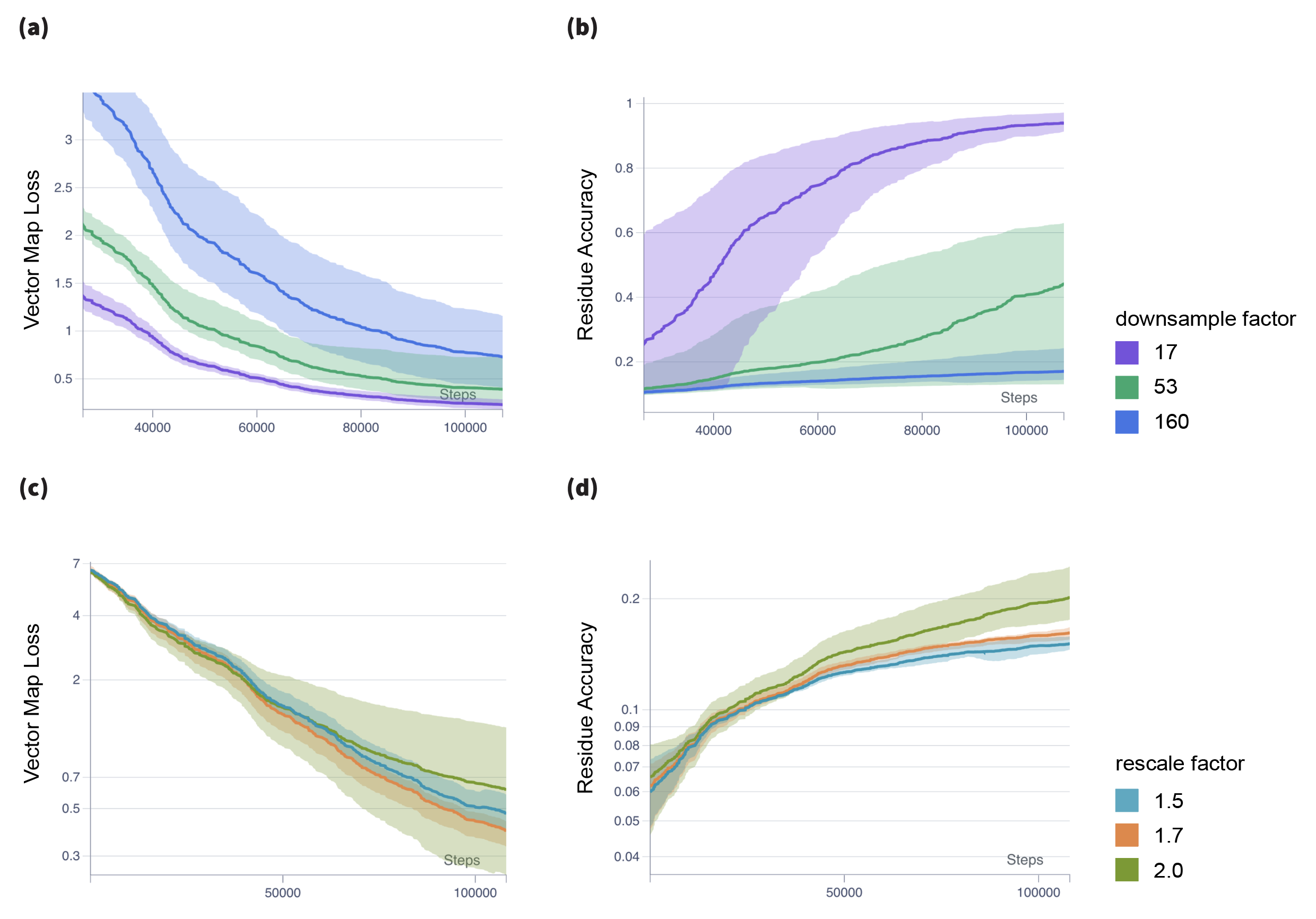
In addition to all-atom ablation found in Table 2 we conducted a similar ablation study on models trained on backbone only atoms as shown in Table 4. We found that backbone only models performed slightly better on backbone reconstruction. Furthermore, in Fig. 9.a we compare the relative vector loss between ground truth coordinates and the coordinates reconstructed from the autoencoder with respect to different downsampling factors. We average over different trials and channel rescale factors. As expected, we find that for lower downsampling factors the structure reconstruction accuracy is better. In Fig 9.b we similarly plot the residue recovery accuracy with respect to different downsampling factors. Again, we find the expected result, the residue recovery is better for lower downsampling factors.
Notably, the relative change in structure recovery accuracy with respect to different downsampling factors is much lower compared to the relative change in residue recovery accuracy for different downsampling factors. This suggest our model was able to learn much more efficiently a compressed prior for structure as compared to sequence, which coincides with the common knowledge that sequence has high redundancy in biological proteins. In Fig. 9.c we compare the structure reconstrution accuracy across different channel rescaling factors. Interestingly we find that for larger rescaling factors the structure reconstruction accuracy is slightly lower.
However, since we trained only for 10 epochs, it is likely that due to the larger number of model parameters when employing a larger rescaling factor it would take somewhat longer to achieve similar results. Finally, in Fig. 9.d we compare the residue recovery accuracy across different rescaling factors. We see that for higher rescaling factors we get a higher residue recovery rate. This suggests that sequence recovery is highly dependant on the number of model parameters and is not easily capturable by efficient structural models.
| Factor | Channels/Layer | # Params [1e6] | C-RMSD (Å) | GDT-TS | GDT-HA |
|---|---|---|---|---|---|
| 17 | [16, 24, 36] | 0.34 | 0.81 0.31 | 96 3 | 81 5 |
| 17 | [16, 27, 45] | 0.38 | 0.99 0.45 | 95 3 | 81 6 |
| 17 | [16, 32, 64] | 0.49 | 1.03 0.42 | 92 4 | 74 6 |
| 53 | [16, 24, 36, 54] | 0.49 | 0.99 0.38 | 92 5 | 74 8 |
| 53 | [16, 27, 45, 76] | 0.67 | 1.08 0.40 | 91 6 | 71 8 |
| 53 | [16, 32, 64, 128] | 1.26 | 1.02 0.64 | 92 9 | 75 11 |
| 160 | [16, 24, 36, 54, 81] | 0.77 | 1.33 0.42 | 84 7 | 63 8 |
| 160 | [16, 27, 45, 76, 129] | 1.34 | 1.11 0.29 | 89 4 | 69 7 |
| 160 | [16, 32, 64, 128, 256] | 3.77 | 0.90 0.44 | 94 7 | 77 9 |
Appendix E Latent Space Analysis
E.1 Visualization of Latent Space
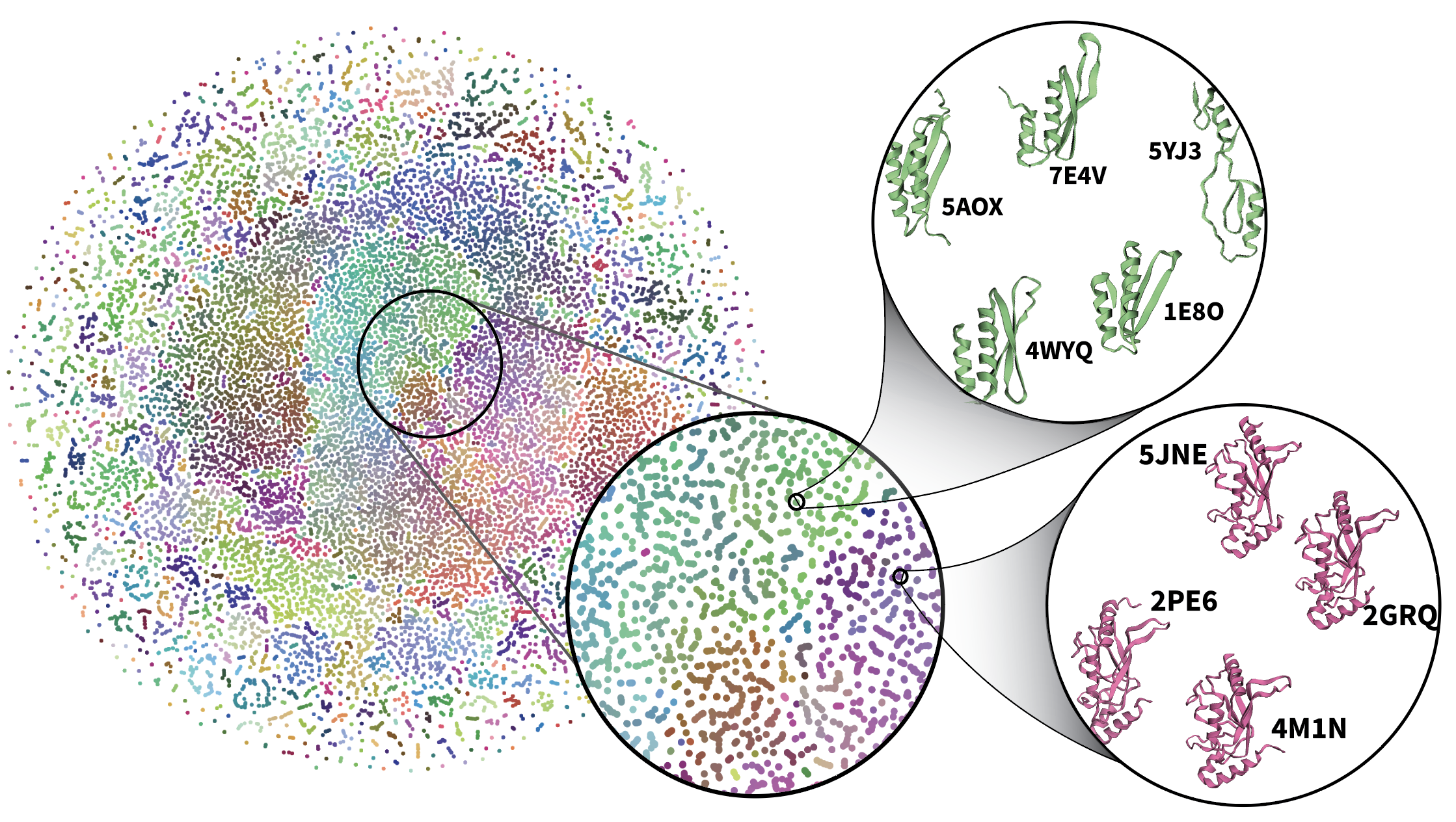
To visualize the learned latent space of Ophiuchus, we forward 50k samples from the training set through a large 485-length model (Figure 10). We collect the scalar component of bottleneck representations, and use t-SNE to produce 2D points for coordinates. We similarly produce 3D points and use those for coloring. The result is visualized in Figure 10. Visual inspection of neighboring points reveals unsupervised clustering of similar folds and sequences.
Appendix F Latent Diffusion Details
We train all Ophiuchus diffusion models with learning rate for 10,000 epochs. For denoising networks we use Self-Interactions with the chunked-channel tensor square operation (Alg. 3).
Our tested models are trained on two different datasets. The MiniProtein scaffolds dataset consists of 66k all-atom structures of sequence length between 50 and 65, and composes of diverse folds and sequences across 5 secondary structure topologies, and is introduced by [Cao et al. (2022)]. We also train a model on the data curated by [Yim et al. (2023)], which consists of approximately 22k proteins, to compare Ophiuchus to the performance of FrameDiff and RFDiffusion in backbone generation for proteins up to 485 residues.
F.1 Self-Consistency Scores
To compute the scTM scores, we recover 8 sequences using ProteinMPNN for 500 sampled backbones from the tested diffusion models. We used a sampling temperature of 0.1 for ProteinMPNN. Unlike the original work, where the sequences where folded using AlphaFold2, we use OmegaFold [Wu et al. (2022b)] similar to [Lin & AlQuraishi (2023)]. The predicted structures are aligned to the original sampled backbones and TM-Score and RMSD is calculated for each alignment. To calculate the diversity measurement, we hierarchically clustered samples using MaxCluster. Diversity is defined as the number of clusters divided by the total number of samples, as described in [Yim et al. (2023)].
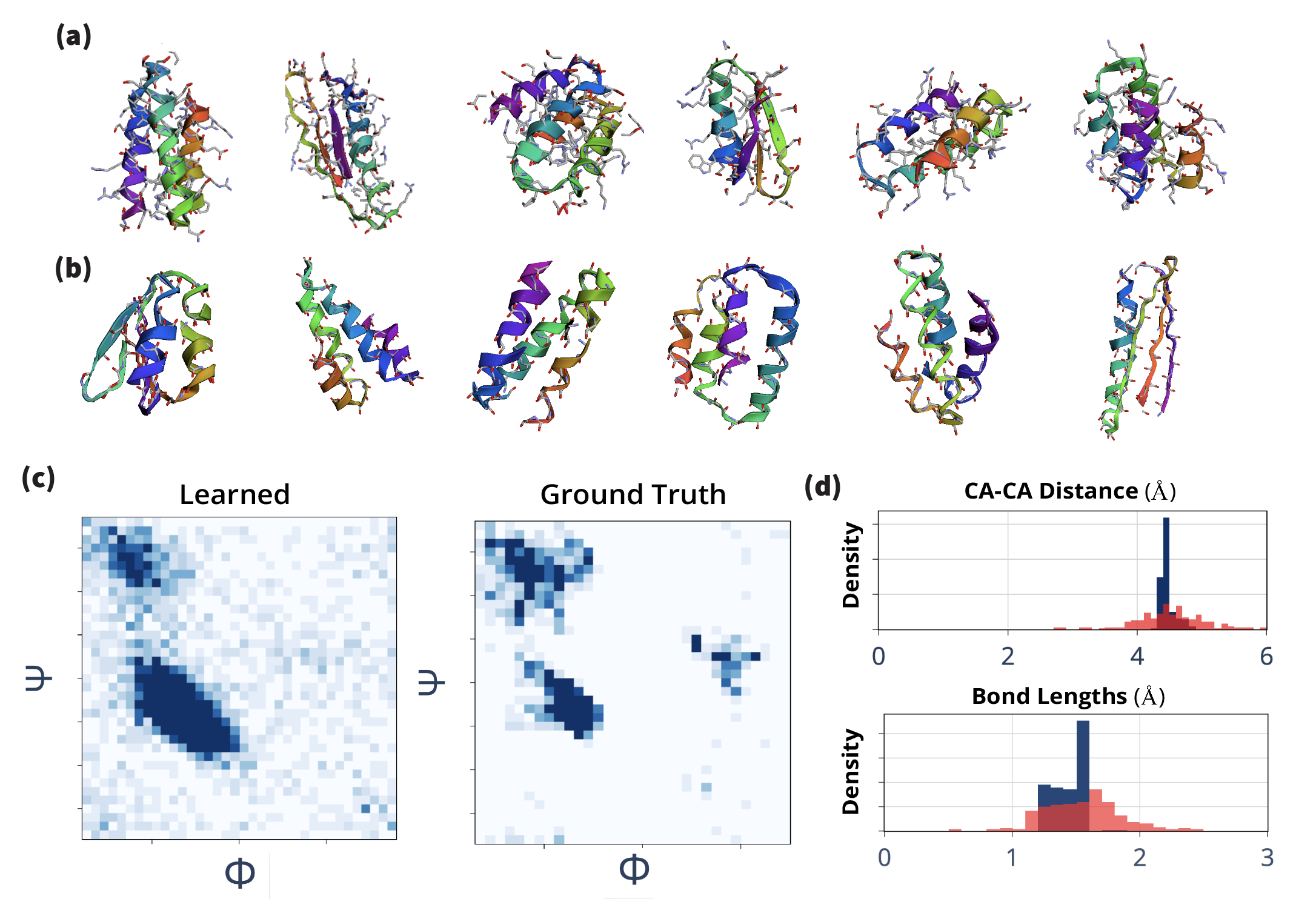
F.2 MiniProtein Model
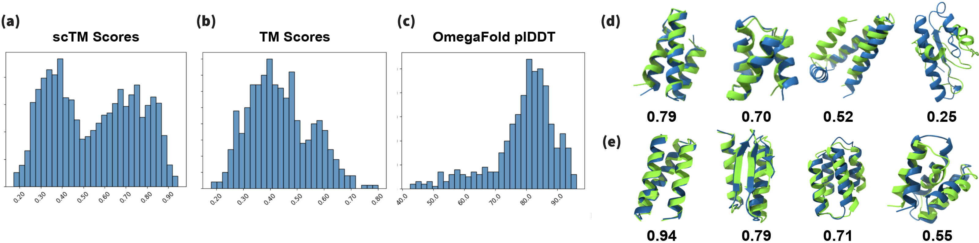
In Figure (13) we show generated samples from our miniprotein model, and compare the marginal distribution of our predictions and ground truth data. In Figure (14.b) we show the distribution of TM-scores for joint sampling of sequence and all-atom structure by the diffusion model. We produce marginal distributions of generated samples Fig.(14.e) and find them to successfully approximate the densities of ground truth data. To test the robustness of joint sampling of structure and sequence, we compute self-consistency TM-Scores[Trippe et al. (2023)]. 54% of our sampled backbones have scTM scores > 0.5 compared to 77.6% of samples from RFDiffusion. We also sample 100 proteins between 50-65 amino acids in 0.21s compared to 11s taken by RFDiffusion on a RTX A6000.
F.3 Backbone Model
We include metrics on designability in Figure 12.
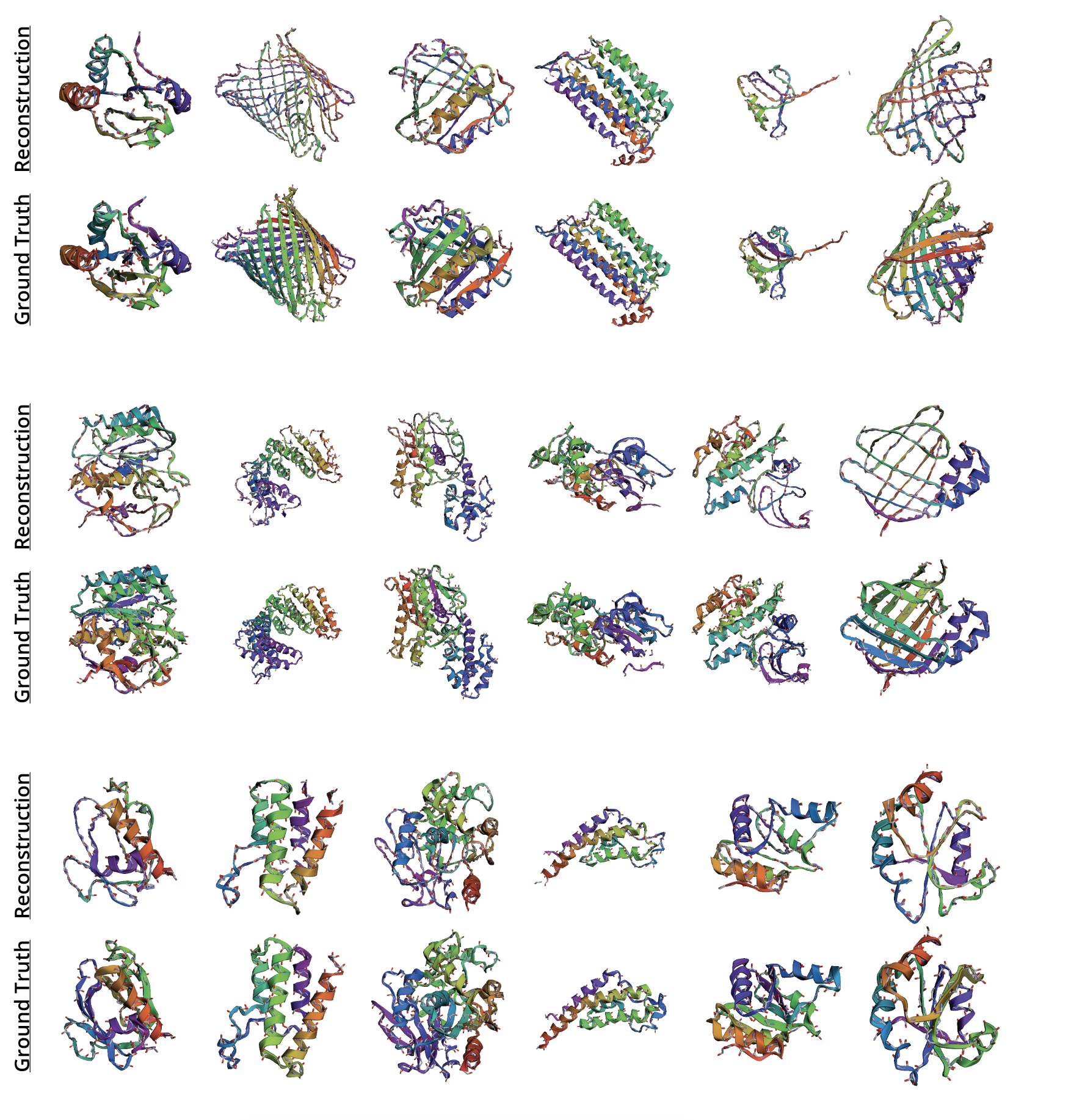
Appendix G Visualization of All-Atom Reconstructions
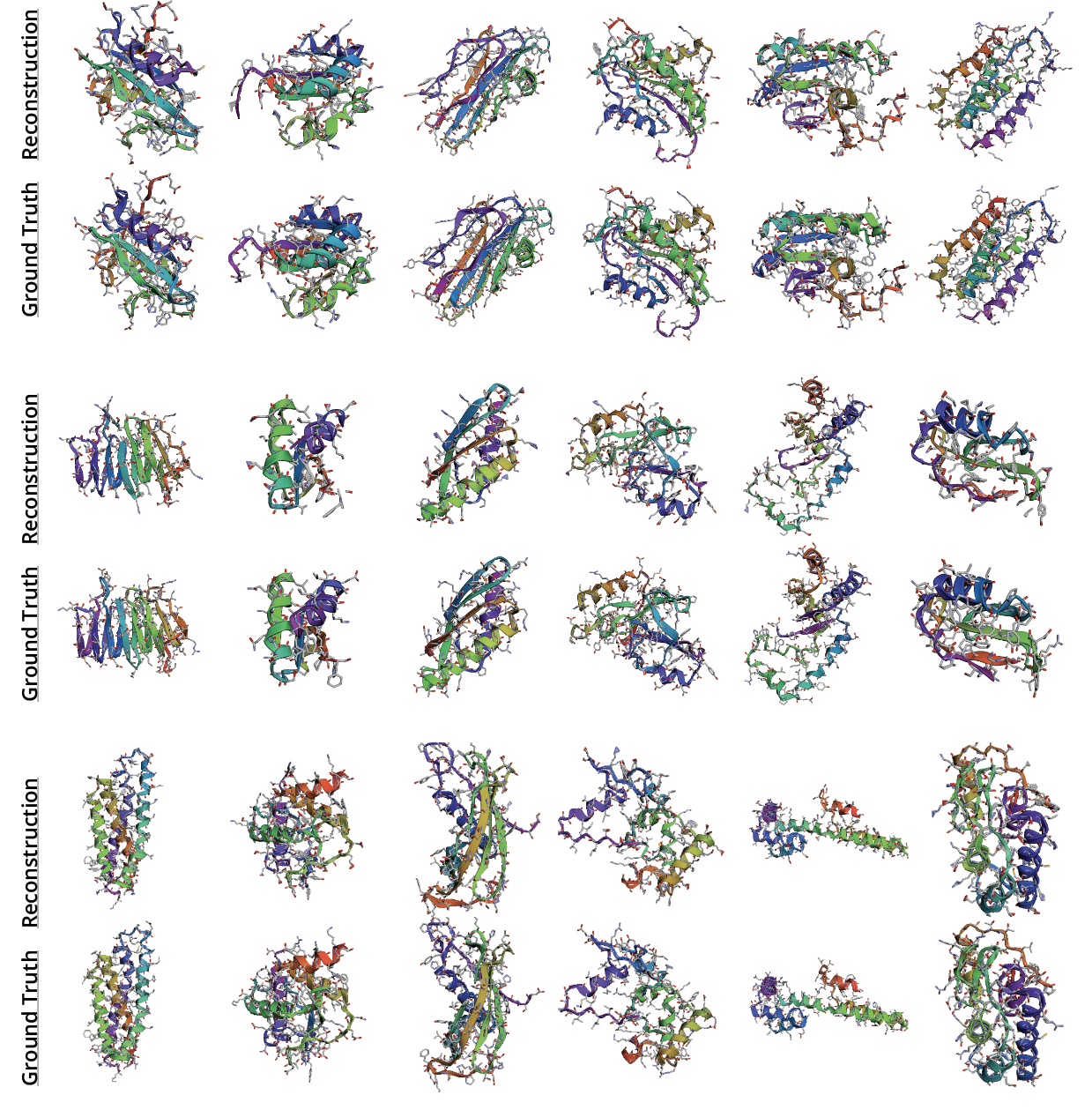
Appendix H Visualization of Backbone Reconstructions
Appendix I Visualization of Random Backbone Samples