Optimal circular dichroism sensing with quantum light: Multi-parameter estimation approach

Illuminating a chiral medium with either LCP or RCP light results in transmission ($T$), reflection ($R$), and absorption ($A$) into the individual polarization modes. The intensity ratios are denoted by $T_{jk}$, $R_{jk}$, and $A_{k}$ for $j,k\in\{\text{L},\text{R}\}$, with the constraint $\sum_{j}(T_{jk}+R_{jk})+A_{k}=1$, where the subscript $k$ ($j$) denotes the input (output) polarization. Apart from absorbance CD that can be quantified by the differential absorption, i.e., $A_{\text{L}}-A_{\text{R}}$, various alternative quantities can be measured to quantify the CD. A typical example would be transmission CD (TCD) defined as $T_{\text{LL}}-T_{\text{RR}}$ Plum et al. (2008) or reflection CD defined as $R_{\text{LL}}-R_{\text{RR}}$ Plum et al. (2016). A polarization conversion in transmission or reflection may also occur, i.e., $T_{jk}\neq 0$ and $R_{jk}\neq 0$ for $j\neq k$, when the three-fold rotational symmetry does not hold with respect to the direction of incidence Menzel et al. (053811). It finally causes circular conversion dichroism, i.e., $T_{\text{LR}}\neq T_{\text{RL}}$ Schwanecke et al. (2008).

In this work, not just for practical relevance with respect to realistic molecular samples or metamaterials that are typically considered, but also to eliminate the linear birefringence leading to unwanted polarization conversion, we focus on chiral media that preserve the four-fold rotational symmetry, for which $T_{jk}=0$ for $j\neq k$ and $R_{jj}=0$ for all $j$ Kwon et al. (2008); Plum et al. (2009); Saba et al. (2013); Khan et al. (2019). When illuminating media with a four-fold symmetry at normal incidence, the reciprocity further imposes $R_{\text{LR}}=R_{\text{RL}}$ Bai et al. (2007); Kaschke et al. (2014). Consequently, we have $T_{\text{LL}}-T_{\text{RR}}=A_{\text{R}}-A_{\text{L}}$, and the intensity difference of the transmitted LCP ($I_{\text{L}}$) and RCP ($I_{\text{R}}$) becomes the key quantity of interest to be measured in usual CD measurement as illustrated in Fig. 1(a). Note that this is not a restrictive scenario but generally valid in usual scenarios when chiral molecules in solution are randomly oriented relative to the incident field. Considering a more general type of measurement that does not directly yield a parameter value under study, we use an estimator to estimate the quantity of TCD, defined as $\Gamma_{-}\equiv T_{\text{L}}-T_{\text{R}}$, where $T_{j}\equiv T_{jj}$.

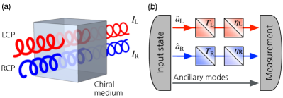
For the quantum mechanical description of CD or TCD sensing, let us consider, for generality, an ancilla-assisted scheme as shown in Fig. 1(b). The scheme consists of the two signal modes $\hat{a}_{\text{L}}$ and $\hat{a}_{\text{R}}$ that correspond to LCP and RCP modes, respectively and arbitrary number of ancillary modes. Such a general setup allows to consider correlated input states among the signal modes and ancillary modes, when necessary. The transmission of each signal mode is described by a beam splitter with transmittance $T_{\text{L (R)}}$. An extra loss that occurs outside an analyte (e.g., non-unity channel transmission or detection efficiency) can also be described by another beam splitter with transmittance $\eta_{\text{L (R)}}$ Loudon (2000). For calculation of the output state, the two consecutive beam splitters in each signal mode can be treated as a single beam splitter, but the transmittances $T_{j}$ and $\eta_{j}$ have to be kept separate because only the parameters $T_{j}$ are of interest in sensing while the factors $\eta_{j}$ degrade the sensing performance. We also assume that the ancilla modes are lossless, which can be held in a controlled manner in many scenarios. The associated input-output relation for the signal mode $j\in\{\text{L},\text{R}\}$ is written as

$\displaystyle\hat{a}_{j}\rightarrow\sqrt{T_{j}\eta_{j}}\hat{a}_{j}+\sqrt{\eta_{j}(1-T_{j})}\hat{b}_{j}+\sqrt{(1-\eta_{j})(1-T_{j})}\hat{c}_{j},$

(1)

where $\hat{b}_{j}$ and $\hat{c}_{j}$ are virtual input modes associated with the chiral medium and the system loss respectively. Equation (1) is applied to the two signal modes of the total input state $|\Psi_{\text{in}}\rangle$ containing ancillary modes. The resultant output state $\hat{\rho}_{\text{out}}$ is measured using a chosen quantum measurement, yielding the outcomes $\boldsymbol{m}$. From these, the TCD parameter $\Gamma_{-}$ is estimated. This is the general CD sensing scheme we aim to investigate in this work.

The precision of CD sensing, a figure of merit which we consider in this work, can be formulated via quantum multi-parameter estimation theory Szczykulska et al. (2016); Liu et al. (2020). Consider an arbitrary pure state $|\Psi_{\text{in}}\rangle$ as an input and suppose that the two transmittance parameters, ${\boldsymbol{T}}=(T_{\text{L}},T_{\text{R}})^{\text{T}}$, shall be estimated by an unbiased estimator from the measurement results ${\boldsymbol{m}}$ that have been drawn from a conditional probability $p({\boldsymbol{m}}|{\boldsymbol{T}})$. In this case, one can find that the $2\times 2$ covariance matrix $\text{Cov}({\boldsymbol{T}})=\langle({\boldsymbol{T}}-\langle{\boldsymbol{T}}\rangle)({\boldsymbol{T}}-\langle{\boldsymbol{T}}\rangle)^{\text{T}}\rangle$ obeys

$\displaystyle\text{Cov}({\boldsymbol{T}})\geq\frac{{\boldsymbol{F}}^{-1}}{\nu},$

(2)

where $\nu$ is the number of measurements being repeated and ${\boldsymbol{F}}$ is the Fisher information matrix (FIM) defined as Helstrom (1976); Paris (2009)

$\displaystyle{\boldsymbol{F}}=\begin{pmatrix}F_{\text{LL}}&F_{\text{LR}}\\ F_{\text{RL}}&F_{\text{RR}}\end{pmatrix},$

(3)

where the matrix elements are written as

$\displaystyle F_{jk}=\sum_{{\boldsymbol{m}}}\frac{1}{p({\boldsymbol{m}}|{\boldsymbol{T}})}\frac{\partial p({\boldsymbol{m}}|{\boldsymbol{T}})}{\partial T_{j}}\frac{\partial p({\boldsymbol{m}}|{\boldsymbol{T}})}{\partial T_{k}},$

(4)

where $j,k\in\{R,L\}$. The lower bound in Eq. (2) is called Cramér-Rao (CR) bound and can always be saturated by a maximum likelihood method in the limit of large $\nu$ Braunstein (1992). The CR bound can be further reduced via optimization of a measurement setting, leading to Helstrom (1976); Paris (2009)

$\displaystyle\text{Cov}({\boldsymbol{T}})\geq\frac{{\boldsymbol{F}}^{-1}}{\nu}\geq\frac{{\boldsymbol{H}}^{-1}}{\nu},$

(5)

where ${\boldsymbol{H}}$ denotes the QFIM defined by

$\displaystyle H_{jk}=\text{Tr}\left[\hat{\rho}_{\boldsymbol{T}}\frac{\hat{\cal L}_{j}\hat{\cal L}_{k}+\hat{\cal L}_{k}\hat{\cal L}_{j}}{2}\right],$

(6)

with $\hat{\cal L}_{j}$ being a symmetric logarithmic derivative (SLD) operator associated with mode $j$ Braunstein and Caves (1994). It is a solution of the equation

$\displaystyle\frac{\partial\hat{\rho}_{\boldsymbol{T}}}{\partial T_{j}}=\frac{1}{2}\left(\hat{\rho}_{\boldsymbol{T}}\hat{\cal L}_{j}+\hat{\cal L}_{j}\hat{\rho}_{\boldsymbol{T}}\right)$

(7)

for the parameter-encoded output state $\hat{\rho}_{\boldsymbol{T}}$. Here, ${\boldsymbol{F}}^{-1}$ and ${\boldsymbol{H}}^{-1}$ are understood as the inverse on their support if the matrices are singular, i.e., not invertible W. Ge et al. (2018). Since the independent SLD operators $\hat{\cal L}_{\text{L}}$ and $\hat{\cal L}_{\text{R}}$ commute, the optimal measurement setting can be constructed over the common eigenbasis of the commuting SLD operators Baumgratz and Datta (2016). Thus, the lower bound in Eq. (5), called QCR bound, is saturable in CD sensing Matsumoto (2002).

Decomposing the state into the diagonalized bases, i.e., $\hat{\rho}_{\boldsymbol{T}}=\sum_{n}p_{n}\left|{\psi_{n}}\right\rangle\left\langle{\psi_{n}}\right|$ with $\langle\psi_{n}|\psi_{m}\rangle=\delta_{n,m}$, one can write the SLD operator as

$\displaystyle\hat{\cal L}_{j}$

$\displaystyle=\sum_{n}\frac{\partial_{j}p_{n}}{p_{n}}\left|{\psi_{n}}\right\rangle\left\langle{\psi_{n}}\right|+2\sum_{n\neq m}\frac{p_{n}-p_{m}}{p_{n}+p_{m}}\langle\psi_{m}|\partial_{j}\psi_{n}\rangle\left|{\psi_{m}}\right\rangle\left\langle{\psi_{n}}\right|,$

(8)

where summation runs over $n,m$ for which $p_{n}+p_{m}\neq 0$ and $\partial_{j}\equiv\partial/\partial T_{j}$ for $j\in\{\text{L},\text{R}\}$. Particularly when $|\partial_{j}\psi_{n}\rangle=0$, the SDL operator $\hat{\cal L}_{j}$ of Eq. (8) becomes $\hat{\cal L}_{j}=\sum_{n}(p_{n})^{-1}(\partial_{j}p_{n})\left|{\psi_{n}}\right\rangle\left\langle{\psi_{n}}\right|$, for which the bases $\{\left|{\psi_{n}}\right\rangle\left\langle{\psi_{n}}\right|\}$ constitute the set of the optimal measurement bases Paris (2009).

An alternative way to find the QFIM is to use the relation between Bures distance ${\cal D}_{\text{B}}^{2}$ Bures (1969); Braunstein and Caves (1994); Facchi et al. (2010), quantum fidelity ${\cal F}$ Uhlmann (1976); Jozsa (1994), and QFIM. In our case, the QFIM $H_{jk}$ is related to the Bures distance ${\cal D}_{\text{B}}^{2}$ for the infinitesimally close states $\hat{\rho}_{\boldsymbol{T}}$ and $\hat{\rho}_{\boldsymbol{T}+\text{d}\boldsymbol{T}}$. It can be written as Liu et al. (2020)

$\displaystyle\sum_{j,k\in\{\text{L},\text{R}\}}H_{jk}\text{d}T_{j}\text{d}T_{k}=4{\cal D}_{\text{B}}^{2}(\hat{\rho}_{\boldsymbol{T}},\hat{\rho}_{\boldsymbol{T}+\text{d}\boldsymbol{T}}),$

(9)

where the Bures distance can be written in terms of quantum fidelity as

$\displaystyle{\cal D}_{\text{B}}^{2}(\hat{\rho}_{\boldsymbol{T}},\hat{\rho}_{\boldsymbol{T}+\text{d}\boldsymbol{T}})=2\left[1-\sqrt{{\cal F}(\hat{\rho}_{\boldsymbol{T}},\hat{\rho}_{\boldsymbol{T}+\text{d}\boldsymbol{T}})}\right]$

(10)

and the quantum fidelity is defined as

$\displaystyle{\cal F}(\hat{\rho}_{\boldsymbol{T}},\hat{\rho}_{\boldsymbol{T}+\text{d}\boldsymbol{T}})=\left(\text{Tr}\sqrt{\sqrt{\hat{\rho}_{\boldsymbol{T}}}\hat{\rho}_{\boldsymbol{T}+\text{d}\boldsymbol{T}}\sqrt{\hat{\rho}_{\boldsymbol{T}}}}\right)^{2}.$

(11)

Thus, the calculation of quantum fidelity leads to the calculation of QFIM.

The matrix inequality of Eq. (5) reads

$\displaystyle{\boldsymbol{n}}^{\text{T}}\text{Cov}(\boldsymbol{T}){\boldsymbol{n}}\geq\frac{{\boldsymbol{n}}^{\text{T}}{\boldsymbol{F}}^{-1}{\boldsymbol{n}}}{\nu}\geq\frac{{\boldsymbol{n}}^{\text{T}}{\boldsymbol{H}}^{-1}{\boldsymbol{n}}}{\nu},$

(12)

for an arbitrary two-dimensional real vector ${\boldsymbol{n}}$ Pezze et al. (2017). This applies when a global parameter $\Gamma=\sum_{j}n_{j}T_{j}$, defined as a linear combination of multiple parameters, is estimated Rubio et al. (2020); Knott et al. (2016); Guo et al. (2020); Oh et al. (2020); Gross and Caves (2020). For CD sensing, $\Gamma_{-}=\boldsymbol{n}^{\text{T}}\boldsymbol{T}$ with $\boldsymbol{n}=(1,-1)$, so we write ${\boldsymbol{n}}^{\text{T}}\text{Cov}(\boldsymbol{T}){\boldsymbol{n}}\equiv\text{Var}(\Gamma_{-})$. From now on, let us drop $\nu$ as it appears everywhere.

In the next sections, we use the QCR bound to investigate the lower bounds to the estimation uncertainty or equivalently, the precision of CD sensing for various input states of light. Individual cases are compared with the UQL which we shall derive below. One can see then what kinds of quantum states can achieve the UQL with and without assistance of ancillary modes. Furthermore, the QCR bounds and the UQL are also compared with the CR bounds for a particular measurement setting we choose depending on the input state considered. this constitutes an explicit specification of the measurement achieving the UQL.

To derive for referential purposes the optimal QCR bound that is obtainable by using only classical light, let us consider a product of coherent states as an input state in Fig. 1(b), i.e., $|\alpha_{\text{L}}\rangle|\alpha_{\text{R}}\rangle=\hat{D}_{\text{L}}(\alpha_{\text{L}})\hat{D}_{\text{R}}(\alpha_{\text{R}})|0\rangle|0\rangle$ in a direct sensing configuration for simplicity, but without loss of generality. The coherent states are characterized by the average photon number $N_{j}=|\alpha_{j}|^{2}$ and the displacement operators are represented by $\hat{D}_{j}(\alpha_{j})=\exp[\alpha\hat{a}_{j}^{\dagger}-\alpha^{*}\hat{a}_{j}]$. Applying the input-output relation of Eq. (1), the output state can be written as

$\displaystyle|\Psi_{\text{out}}\rangle_{\text{coh}}=|\alpha_{\text{L}}^{\text{(out)}}\rangle|\alpha_{\text{R}}^{\text{(out)}}\rangle$

(13)

with $\alpha_{j}^{\text{(out)}}=\sqrt{\eta_{j}T_{j}}\alpha_{j}$. For such a pure output state, the QFIM of Eq. (6) can be calculated via Paris (2009); Knott et al. (2016); Baumgratz and Datta (2016)

$\displaystyle H_{jk}$

$\displaystyle=\frac{1}{2}\langle\Psi_{\text{out}}|\left(\hat{\cal L}_{j}\hat{\cal L}_{k}+\hat{\cal L}_{k}\hat{\cal L}_{j}\right)|\Psi_{\text{out}}\rangle,$

(14)

where the SLD operator $\hat{\cal L}_{j}$ can be written for a pure state $|\Psi_{\text{out}}\rangle$ as

$\displaystyle\hat{\cal L}_{j}=2\partial_{j}|\Psi_{\text{out}}\rangle\langle\Psi_{\text{out}}|.$

(15)

Through some algebraic calculation (see Appendix A for details), one can find that the QFIM for $\boldsymbol{T}$ with a coherent state input is diagonalized and written as

$\displaystyle\boldsymbol{H}_{\text{coh}}=\text{diag}\left(\frac{\eta_{\text{L}}N_{\text{L}}}{T_{\text{L}}},\frac{\eta_{\text{R}}N_{\text{R}}}{T_{\text{R}}}\right).$

(16)

It is clear that $\boldsymbol{H}_{\text{coh}}\rightarrow\boldsymbol{0}$ as $\eta_{\text{L/R}}\rightarrow 0$. By substituting $\boldsymbol{H}_{\text{coh}}$ to Eq. (12), the QCR bound to the estimation uncertainty of $\Gamma_{-}$ can thus be written as

$$\text{Var}(\Gamma_{-})_{\text{coh}}=\frac{T_{\text{L}}}{\eta_{\text{L}}N_{\text{L}}}+\frac{T_{\text{R}}}{\eta_{\text{R}}N_{\text{R}}}.$$

(17)

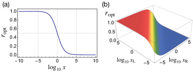
Defining the ratio $r=N_{\text{L}}/N_{\text{tot}}$ for the total average intensity in the signal modes $N_{\text{tot}}=N_{\text{L}}+N_{\text{R}}$, which we fix throughout this work as a constraint, we find that the optimal ratio can be written as

$\displaystyle r_{\text{opt}}=\frac{1}{1+\sqrt{\frac{\eta_{\text{L}}T_{\text{R}}}{\eta_{\text{R}}T_{\text{L}}}}},$

(18)

for which the QCR bound of Eq. (17) is minimized and thus reads

$\displaystyle\text{Var}(\Gamma_{-})_{\text{coh}}^{\text{opt}}=\frac{1}{N_{\text{tot}}}\left(\sqrt{\frac{T_{\text{L}}}{\eta_{\text{L}}}}+\sqrt{\frac{T_{\text{R}}}{\eta_{\text{R}}}}\right)^{2}.$

(19)

The optimal ratio $r_{\text{opt}}~{}$ of Eq. (18) is presented in Fig. 2(a) as a function of $\eta_{\text{L}}T_{\text{R}}/\eta_{\text{R}}T_{\text{L}}~{}$ in log scale, while shown in Fig. 2(b) as a function of $T_{\text{L}}$ and $T_{\text{R}}$ in log scale for balanced losses, i.e., $\eta_{\text{L}}=\eta_{\text{R}}$. They clearly show that more energy needs to be injected into a more lossy signal mode to keep the optimal intensity balance between the signal modes, written as

$\displaystyle N_{\text{L}}:N_{\text{R}}=\sqrt{\frac{T_{\text{L}}}{\eta_{\text{L}}}}:\sqrt{\frac{T_{\text{R}}}{\eta_{\text{R}}}}.$

(20)

In most cases, the difference in transmission between LCP and RCP light is extremely small and in good approximation it can be assumed that they are close to equal, i.e., $T_{j}=T_{k}$. Provided losses are balanced $\eta_{j}=\eta_{k}$, the same amount of energies, i.e., $N_{\text{L}}=N_{\text{R}}$, would be, to a very good approximation, the optimal choice in a classical sensing scheme, for which $\text{Var}(\Gamma_{-})_{\text{coh}}^{\text{opt}}=4T/\eta N_{\text{tot}}$ with $T\equiv T_{\text{L/R}}$ and $\eta\equiv\eta_{\text{L/R}}$. In cases where the two transmittances cannot be assumed to be equal, our findings can be combined with an adaptive scheme Valeri et al. ; Nolan et al. . There, the input energies between LCP and RCP modes are adjusted in real-time, based on a prior information about the parameter being updated over repetition of the measurement.

One could consider an ancilla-assisted configuration with classically correlated coherent state input that can be written as

$\displaystyle\hat{\rho}_{\text{coh}}=\int p(\alpha_{\text{L}},\alpha_{\text{R}},\alpha_{\text{A}})|\alpha_{\text{L}},\alpha_{\text{R}},\alpha_{\text{A}}\rangle\langle\alpha_{\text{L}},\alpha_{\text{R}},\alpha_{\text{A}}|\text{d}\alpha_{\text{L}}\text{d}\alpha_{\text{R}}\text{d}\alpha_{\text{A}}$

(21)

with $\text{Tr}[\hat{a}^{\dagger}_{j}~{}\hat{a}_{j}\hat{\rho}_{\text{coh}}]=N_{j}$. Applying the convexity of the QFIM Takeoka et al. (2017), one can prove that the QCR bound to be obtained for the input of Eq. (21) is always equal to or greater than the CB of Eq. (19). Therefore, neither ancillary modes nor classical correlation are useful here.

Let us now derive the UQL on the estimation uncertainty of the TCD parameter $\Gamma_{-}$. When $\eta_{\text{L/R}}=1$, the maximum QFIM for two intensity parameters $(T_{\text{L}},T_{\text{R}})$, optimized over all input states, has been found in Ref. Nair (2018) and can be written as

$\displaystyle{\boldsymbol{H}}_{\text{max}}^{\text{lossless}}=\text{diag}\left(\frac{N_{\text{L}}}{T_{\text{L}}(1-T_{\text{L}})},\frac{N_{\text{R}}}{T_{\text{R}}(1-T_{\text{R}})}\right).$

(22)

It has been shown that the QCR bound associated with ${\boldsymbol{H}}_{\text{max}}^{\text{lossless}}$ can be achieved in general by so-called number-diagonal signal states in ancilla-assisted scheme Nair (2018) or by Fock state input without ancilla modes when $N_{\text{L}}$ and $N_{\text{R}}$ are integers Adesso et al. (2009).

In the presence of loss (i.e., $\eta_{\text{L/R}}\neq 1$), the SLD operators $\hat{\cal L}_{j}$ for Eq. (22) is modified to $\hat{\cal S}_{j}$, written as (see Appendix B for details)

$\displaystyle\hat{\cal S}_{j}=\eta_{j}\hat{\cal L}_{j},$

(23)

for $j\in\{\text{L},\text{R}\}$. This leads ${\boldsymbol{H}}_{\text{max}}^{\text{lossless}}$ of Eq. (22) to be written as

$\displaystyle{\boldsymbol{H}}_{\text{max}}=\text{diag}\left(\frac{\eta_{\text{L}}N_{\text{L}}}{T_{\text{L}}(1-\eta_{\text{L}}T_{\text{L}})},\frac{\eta_{\text{R}}N_{\text{R}}}{T_{\text{R}}(1-\eta_{\text{R}}T_{\text{R}})}\right).$

(24)

This is the maximum QFIM for two intensity parameters $(T_{\text{L}},T_{\text{R}})$ in the presence of loss. It is clear that ${\boldsymbol{H}}_{\text{max}}\rightarrow\boldsymbol{0}$ as $\eta_{\text{L/R}}\rightarrow 0$.

The UQL to the estimation uncertainty $\text{Var}(\Gamma_{-})$ can be readily obtained by substituting Eq. (24) into Eq. (12), resulting in

$\displaystyle\text{Var}(\Gamma_{-})_{\text{UQL}}=\frac{T_{\text{L}}(1-\eta_{\text{L}}T_{\text{L}})}{\eta_{\text{L}}N_{\text{L}}}+\frac{T_{\text{R}}(1-\eta_{\text{R}}T_{\text{R}})}{\eta_{\text{R}}N_{\text{R}}}.$

(25)

This is the UQL to the estimation uncertainty or equivalently the precision of CD sensing for arbitrarily given $N_{\text{L}}$ and $N_{\text{R}}$. The SLD operator $\hat{\cal L}_{-}$ for the parameter $\Gamma_{-}$ is obtained by using Eq. (7) and

$\displaystyle\frac{\partial\hat{\rho}_{\boldsymbol{T}}}{\partial\Gamma_{-}}=\frac{1}{2}\left(\hat{\rho}_{\boldsymbol{T}}\hat{\cal L}_{-}+\hat{\cal L}_{-}\hat{\rho}_{\boldsymbol{T}}\right).$

(26)

It can thus be shown to be

$\displaystyle\hat{\cal L}_{-}=\frac{1}{2}\left(\hat{\cal S}_{\text{L}}-\hat{\cal S}_{\text{R}}\right).$

(27)

One can easily show that the optimal ratio $r_{\text{opt}}$ that minimizes $\text{Var}(\Gamma_{-})_{\text{UQL}}$ of Eq. (25) can be written as

$\displaystyle r_{\text{opt}}=\frac{1}{1+\sqrt{\frac{\eta_{\text{L}}T_{\text{R}}(1-\eta_{\text{R}}T_{\text{R}})}{\eta_{\text{R}}T_{\text{L}}(1-\eta_{\text{L}}T_{\text{L}})}}},$

(28)

for which

$\displaystyle\text{Var}(\Gamma_{-})_{\text{UQL}}^{\text{opt}}=\frac{1}{N_{\text{tot}}}\left(\sqrt{\frac{T_{\text{L}}(1-\eta_{\text{L}}T_{\text{L}})}{\eta_{\text{L}}}}+\sqrt{\frac{T_{\text{R}}(1-\eta_{\text{R}}T_{\text{R}})}{\eta_{\text{R}}}}\right)^{2}.$

(29)

This is the UQL to the precision of CD sensing for the optimal raio between $N_{\text{L}}$ and $N_{\text{R}}$. It is obtained by the optimal input whose signal modes satisfying the optimal intensity ratio of Eq. (28) and the optimal measurement setting. The UQL applies to both cases with and without ancillary modes. Furthermore, the optimal schemes for scenarios without excess loss found in Ref. Nair (2018) can be used to reach the UQL of Eq. (29) in lossy scenarios.

Comparing the UQL of Eq. (29) with the CB of Eq. (19), one can see that the quantum enhancement is achieved by the factors of $(1-\eta_{\text{L}}T_{\text{L}})$ and $(1-\eta_{\text{R}}T_{\text{R}})$ in the numerator of the respective terms, but diminishes with loss, i.e., as $\eta_{\text{L/R}}\rightarrow 0$. Note that both QCR bounds of Eqs. (19) and (29) scale with $N_{\text{tot}}$, i.e., following the shot-noise scaling in terms of the total energy $N_{\text{tot}}$, as in the single loss parameter estimation case Adesso et al. (2009). The optimal ratio $r_{\text{opt}}$ of Eq. (28) exhibits the same behavior as shown in Figs. 2(a) and (b), but with $\eta_{\text{L}}T_{\text{R}}(1-\eta_{\text{R}}T_{\text{R}})/\eta_{\text{R}}T_{\text{L}}(1-\eta_{\text{L}}T_{\text{L}})~{}$ and $x_{j}=T_{j}(1-\eta_{j}T_{j})$ for $j=\text{L},\text{R}$, respectively. The optimal ratio $r_{\text{opt}}$ can also be understood as the optimal balance of the average intensities between the LCP and RCP modes, written as

$\displaystyle N_{\text{L}}:N_{\text{R}}=\sqrt{\frac{T_{\text{L}}(1-\eta_{\text{L}}T_{\text{L}})}{\eta_{\text{L}}}}:\sqrt{\frac{T_{\text{R}}(1-\eta_{\text{R}}T_{\text{R}})}{\eta_{\text{R}}}}.$

(30)

Again, in most cases, $T_{j}\approx T_{k}$ and $\eta_{j}\approx\eta_{k}$, so the same amount of energies, i.e., $N_{\text{L}}=N_{\text{R}}$, would be the optimal choice in the ultimate CD sensing scheme, for which $\text{Var}(\Gamma_{-})_{\text{UQL}}^{\text{opt}}=4T(1-\eta T)/\eta N_{\text{tot}}$ with $T\equiv T_{\text{L/R}}~{}$ and $\eta\equiv\eta_{\text{L/R}}$. In this case, the quantum enhancement of the UQL as compared to the CB can be quantified by the ratio defined as

$\displaystyle\frac{\text{Var}(\Gamma_{-})_{\text{coh}}^{\text{opt}}}{\text{Var}(\Gamma_{-})_{\text{UQL}}^{\text{opt}}}=\frac{1}{1-\eta T}.$

(31)

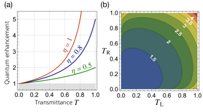
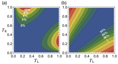
Note that this enhancement factor diverges as $\eta T\rightarrow 1$, so the infinite-fold enhancement can be in principle achieved or a huge quantum enhancement can be exploited in well-controlled situations. The enhancement is degraded as $\eta$ decreases in lossy cases, e.g., the maximal enhancement is only two-fold for $\eta=0.5$. The enhancement factor is presented in Fig. 3(a) as a function of transmittance $T$ for $\eta=1,0.8$, and $0.5$. It clearly shows that the quantum enhancement is sensitive to the loss parameter $\eta$, so reducing the loss in a sensing setup is crucial to increase the quantum enhancement for a given $T_{\text{L}}\approx T_{\text{R}}=T$ in CD sensing. We, nevertheless, stress that the quantum enhancement factor is always greater than unity unless either $\eta$ or $T$ is zero. Figure 3(b) shows an overall quantum enhancement in terms of arbitrary $T_{\text{L}}$ and $T_{\text{R}}$ for balanced loss $\eta=0.8$ chosen as an example.

We now show that the Fock state input $|N_{\text{L}}\rangle|N_{\text{R}}\rangle$ without using ancillary modes can achieve the UQL. Through the beam splitter transformation of Eq. (1), the output state can be written as

$\displaystyle\hat{\rho}_{\text{Fock}}=\sum_{m_{\text{L}},m_{\text{R}}}p(m_{\text{L}},m_{\text{R}}|\boldsymbol{T})|m_{\text{L}},m_{\text{R}}\rangle\langle m_{\text{L}},m_{\text{R}}|,$

(32)

where

$\displaystyle p(m_{\text{L}},m_{\text{R}}|\boldsymbol{T})=\prod_{j=\text{L},\text{R}}\binom{N_{j}}{m_{j}}(\eta_{j}T_{j})^{m_{j}}(1-\eta_{j}T_{j})^{N_{j}-m_{j}}.$

(33)

With this, one can show that the QFIM is equal to ${\boldsymbol{H}}_{\text{max}}$ of Eq. (24), finally achieving the UQL of Eq. (29) when the photon numbers $N_{\text{L}}$ and $N_{\text{R}}$ follow the optimal ratio of Eq. (30). Therefore, Fock state input $|N_{\text{L}}\rangle|N_{\text{R}}\rangle$ is the optimal state to reach the UQL to the precision in CD sensing. The UQL is inversely proportional to the total average photon number $N_{\text{tot}}$, so it is recommended to increase the total intensity of an input state while keeping the optimal ratio of Eq. (30). However, large Fock states with $N_{j}\gg 1$ cannot be readily generated with current technology Varcoe et al. (2000); Bertet et al. (2002); Waks et al. (2006). As shown in Ref. Nair (2018), an alternative way is to use $N_{j}$ single-photons Lounis and Orrit ; Eisaman et al. ; Meyer-Scott et al. (2020), which also leads to the UQL on the precision of CD sensing.

Another useful quantum source of light is the so-called twin-beam. They have widely been used in many applications including quantum imaging Genovese (2016), quantum illumination Lloyd (2008); Tan et al. (2008); Lopaeva et al. (2013); Nair and Gu (2020), and quantum sensing Meda et al. (2017) due to the strong photon number correlation Jedrkiewicz et al. (2004); Bondani et al. (2007); Blanchet et al. (2008); Peřina et al. (2012). The twin-beam state can be generated from a spontaneous parametric down conversion process Burnham and Weinberg (1970); Heidmann et al. (1987); Schumaker and Caves (1985) and is formally written as the two-mode squeezed vacuum (TMSV) state,  $|\text{TMSV}\rangle=\hat{S}_{2}(\xi)\left|{00}\right\rangle$ with the two-mode squeezing operator $\hat{S}_{2}(\xi)=\exp[\xi^{*}\hat{a}\hat{b}-\xi\hat{a}^{\dagger}\hat{b}^{\dagger}]$ for $\xi=re^{i\theta}$ with $\{r,\theta\}\in\mathbb{R}$. As shown below, such TMSV states or twin-beams can be used for CD sensing in two ways.

First, let us consider CD sensing scheme using two TMSV states $|\text{TMSV}\rangle\otimes|\text{TMSV}\rangle$ in an ancilla-assisted configuration. Let us assume that the respective signal modes of the TSMV states are sent to LCP and RCP mode, while their respective ancillary modes are held losslessly. Such a setting has been shown to achieve the QFIM of Eq. (22) for $(T_{\text{L}},T_{\text{R}})$ in the absence of additional loss Nair (2018). The analysis in Section III.2 implies that the same setting can be used to achieve the UQL of Eq. (29) when the average intensities of the signal states of the two TMSV states satisfy the optimal ratio of Eq. (30). Therefore, the twin-beam input is the optimal state to reach the UQL to the precision in CD sensing in an ancilla-assisted configuration. One can find other optimal states in ancilla-assisted scheme according to the analysis in Ref. Nair (2018).

A second way to use the TMSV state input is to inject the two modes of a single TMSV state into LCP and RCP modes, respectively. Note that ancillary modes are not considered in such direct sensing scheme and $N_{\text{L}}=N_{\text{R}}=\sinh^{2}r\equiv N$ as an intrinsic feature of the twin-beam state. The output state $\hat{\rho}_{\boldsymbol{T}}$ can be obtained by using the input-output relation of Eq. (1) for the input state $|\text{TMSV}\rangle$. In this particular case, analytical calculation of the QFIM using SLD operators is tricky, so we use the quantum fidelity of Eq. (11) that can be calculated more easily using a closed expression Marian and Marian (2012); Banchi et al. (2015). Leaving all the technical details to Appendix C, we finally have the QFIM written as

	$\displaystyle H_{jj}$	$\displaystyle=\frac{\chi_{j\bar{j}}\eta_{j}N}{T_{j}(1-\eta_{j}T_{j})},$		(34)
	$\displaystyle H_{jk}$	$\displaystyle=\frac{-\eta_{j}\eta_{k}N(N+1)}{1+\eta_{j}T_{j}(1-\eta_{k}T_{k})N+\eta_{k}T_{k}(1-\eta_{j}T_{j})N},$		(35)

with

$\displaystyle\chi_{j\bar{j}}=\frac{1-\eta_{j}T_{j}(1-\eta_{\bar{j}}T_{\bar{j}})+\eta_{\bar{j}}T_{\bar{j}}(1-\eta_{j}T_{j})N}{1+\eta_{j}T_{j}(1-\eta_{\bar{j}}T_{\bar{j}})N+\eta_{\bar{j}}T_{\bar{j}}(1-\eta_{j}T_{j})N},$

(36)

where $j\neq k\in\{\text{L},\text{R}\}$, $\bar{j}=\text{R}$ if $j=\text{L}$, and vice versa.

In comparison with the QFIM of Eq. (24), the diagonal element $H_{jj}$ of Eq. (34) contains the additional factor $\chi_{jk}$ coming from the correlation between the signal modes. One can show that $0\leq\chi_{jk}\leq 1$ holds, where the upper bound is reached when $\eta_{j}T_{j}=0$ or $\eta_{k}T_{k}=1$, while the lower bound is obtained when $\eta_{j}T_{j}=1$ and $\eta_{k}T_{k}=0$. The QCR bound for the estimation uncertainty $\text{Var}(\Gamma_{-})$ can thus be written in terms of Eqs. (34) and (35) as

$\displaystyle\text{Var}(\Gamma_{-})_{\text{TMSV}}=\frac{H_{\text{LL}}+H_{\text{RR}}+H_{\text{LR}}+H_{\text{RL}}}{H_{\text{LL}}H_{\text{RR}}-H_{\text{LR}}H_{\text{RL}}}.$

(37)

It can be easily shown that the use of a TMSV state input in direct sensing scheme cannot achieve the UQL to the precision of CD sensing. However, one can find that the QCR bound $\text{Var}(\Gamma_{-})_{\text{TMSV}}$ of Eq. (37) becomes similar to the UQL at some regimes of parameters, which we elaborate on in more details below.

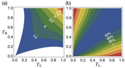
For comparison of $\text{Var}(\Gamma_{-})_{\text{TMSV}}$ with the other cases, let us set $N_{\text{tot}}=2N=2$ and $\eta_{\text{L}}=\eta_{\text{R}}=0.8$ as example without loss of generality. In Fig. 4(a), we show the quantum enhancement $\text{Var}(\Gamma_{-})_{\text{coh}}^{\text{opt}}/\text{Var}(\Gamma_{-})_{\text{TMSV}}$ is limited to only the presented region. Such a beneficial region depends on the values of $N$ and $\eta_{\text{L (R)}}$, but in a particular region of interest for CD sensing, i.e., when $T_{\text{L}}\approx T_{\text{R}}$, the enhancement is always present and significant. More interestingly and clearly, it can be shown that $\text{Var}(\Gamma_{-})_{\text{TMSV}}=\text{Var}(\Gamma_{-})_{\text{UQL}}^{\text{opt}}$ holds up to the first-order in $\delta T$ for $T_{\text{R}}=T_{\text{L}}+\delta T$ when losses are equally balanced $\eta_{\text{L}}=\eta_{\text{R}}$. Such a feature is evidently shown in Figs. 4(a) and (b) around the region where $T_{\text{L}}\approx T_{\text{R}}$. This indicates that in most cases when $T_{\text{L}}$ and $T_{\text{R}}$ can be assumed in good approximation as equal, one can use the direct sensing scheme with the TMSV state input as a practical scheme. The use of TMSV state input also promises quantum enhancement for any value of $T\equiv T_{\text{L}}=T_{\text{R}}$, as already shown in Fig. 3. This is an important finding as it opens a practical path towards exploiting of practical quantum resources in realistic CD sensing.

It is worth discussing the role of the average photon number $N$ in $\text{Var}(\Gamma_{-})_{\text{TMSV}}$. A noticeable behavior is revealed in the limit of large $N$. Both $\text{Var}(\Gamma_{-})_{\text{UQL}}^{\text{opt}}$ and $\text{Var}(\Gamma_{-})_{\text{coh}}^{\text{opt}}$ approach zero as $N\rightarrow\infty$, whereas $\text{Var}(\Gamma_{-})_{\text{TMSV}}$ becomes

$\displaystyle\text{Var}(\Gamma_{-})_{\text{TMSV}}|_{N\rightarrow\infty}=\frac{(T_{\text{L}}-T_{\text{R}})^{2}(1-\eta_{\text{L}}T_{\text{L}})(1-\eta_{\text{R}}T_{\text{R}})}{1+\eta_{\text{L}}T_{\text{L}}(1-\eta_{\text{R}}T_{\text{R}})+\eta_{\text{R}}T_{\text{R}}(1-\eta_{\text{L}}T_{\text{L}})}.$

(38)

This implies that the use of the TMSV state input outperforms the CB only when $T_{\text{L}}\approx T_{\text{R}}$ or $N$ is small. In other words, as $N$ is reduced, the beneficial region in Fig. 4(c) becomes wider, but never covers the entire region. This means that no quantum enhancement is obtained when either $T_{\text{L}}$ or $T_{\text{R}}$ is too small even in the limit $N\rightarrow 0$. Such a region is of course not of much interest for CD sensing, but could be significant for other applications.

For an estimator of $\hat{\Gamma}_{-}$, one can define the signal-to-noise ratio of an estimate $\Gamma_{-}$ as

$\displaystyle\text{SNR}=\frac{\langle\hat{\Gamma}_{-}\rangle^{2}}{\text{Var}(\Gamma_{-})},$

(39)

where $\langle\hat{\Gamma}_{-}\rangle^{2}=\Gamma_{-}^{2}$ for an unbiased estimator. Using Eq. (12), one can easily show that for a given input state the SNR is upper bounded as

$\displaystyle\text{SNR}\leq\frac{\Gamma_{-}^{2}}{\text{Var}(\Gamma_{-})_{\text{QCR}}},$

(40)

where $\text{Var}(\Gamma_{-})_{\text{QCR}}$ is the QCR bound to $\text{Var}(\Gamma_{-})$. This shows that the upper bound of SNR becomes higher by increasing $\Gamma_{-}$ while decreasing $\text{Var}(\Gamma_{-})_{\text{QCR}}$. In other words, precise sensing with small $\text{Var}(\Gamma_{-})_{\text{QCR}}$ yields high SNR, but its inverse does not hold. This implies that assessment of CD sensing in terms of SNR does not guarantee precise estimation of CD or TCD parameter. The equality in Eq. (40) can be saturated when the optimal measurement setting and the optimal estimator are used for a given state. A similar SNR inequality for a single parameter estimation has also been discussed in Ref. Paris (2009).

For a coherent state input in a direct sensing configuration, the output state is given as Eq. (13) and the probability distribution of detecting $m_{\text{L}}$ and $m_{\text{R}}$ photons at the respective output ports is written as

$\displaystyle p(m_{\text{L}},m_{\text{R}}|\boldsymbol{T})=\prod_{j=\text{L},\text{R}}e^{-\eta_{j}T_{j}N_{j}}\frac{(\eta_{j}T_{j}N_{j})^{m_{j}}}{m_{j}!}.$

(41)

Using Eq. (4), one can show that the FIM with Eq. (41) is the same as QFIM of Eq. (16), implying that the PNRD is the optimal measurement setting to reach the optimal classical bound of Eq. (17) when $N_{\text{L}}$ and $N_{\text{R}}$ are arbitrary chosen or the CB of Eq. (19) when the optimal ratio between $N_{\text{L}}$ and $N_{\text{R}}$ is chosen.

For a Fock state input without ancillary modes, the output state of Eq. (32) is diagonalized over the photon number states $\{|m_{\text{L}},m_{\text{L}}\rangle\}$. It is clear that the diagonalized basis is independent of the parameter $\boldsymbol{T}$, so the second term in Eq. (8) vanishes and consequently the FIM of Eq. (4) is the same as the QFIM of Eq. (24). This indicates that the PNRD offers the optimal measurement setting for the case using Fock state inputs. The optimality of the PNRD can also be proved from the fact that the eigenstates of the corresponding SLD operator are the photon number states $\{|m_{\text{L}},m_{\text{L}}\rangle\}$ Paris (2009); Oh et al. (2019).

When multiple single photons are used Adesso et al. (2009) instead of large Fock states that are yet unavailable with current technology Lounis and Orrit ; Eisaman et al. ; Meyer-Scott et al. (2020), we can use, instead of PNRD, single-photon detectors which are a well-established technology Holzman and Ivry (2019). This achieves the UQL.

When using twin-beams in ancilla-assisted scheme, the QFIM of Eq. (22) has been shown to be achievable by performing PNRD in all the four modes, i.e., two signal and two ancillary modes Nair (2018). As explained previously, such optimality of the measurement scheme also carries over to the measurement of CD in the presence of loss, consequently achieving the UQL.

To reach the same bound, one can use $M=N/n$ copies of weakly squeezed TMSVs with the average photon number of $n\ll 1$ on each mode and perform direct detection on each two-mode output state Nair (2018). Apart from placing less demands on high squeezing required in the twin-beam, weak fields with $n\ll 1$ allow us to perform, instead of PNRD, single-photon detection Holzman and Ivry (2019).

For direct sensing scheme with a TMSV state input, the output state is a mixed state and not diagonalized over the photon number states. The photon number distribution of the output state is given as

$\displaystyle p(m_{\text{L}},m_{\text{R}}|\boldsymbol{T})=\sum_{n=0}^{\infty}\frac{N^{n}}{(N+1)^{n+1}}\prod_{j=\text{L},\text{R}}f_{j}(n),$

(42)

where $f_{j}(n)=\binom{n}{m_{j}}(\eta_{j}T_{j})^{m_{j}}(1-\eta_{j}T_{j})^{n-m_{j}}$. In this case, we numerically calculate the $\boldsymbol{F}$ of Eq. (4), which gives rise to the CR bound. The latter is compared with the QCR bound $\text{Var}(\Gamma_{-})_{\text{TMSV}}$ and the UQL $\text{Var}(\Gamma_{-})_{\text{UQL}}$ for balanced losses $\eta=0.8$ chosen as an example. They are shown in Figs. 5(a) and (b), respectively. The CR bound is not generally the same as the QCR bound $\text{Var}(\Gamma_{-})_{\text{TMSV}}$, but they become extremely similar when $T_{\text{L}}$ and $T_{\text{R}}$ are close to each other, as shown in Fig. 5(a). This indicates that the CR bound can also be similar the UQL $\text{Var}(\Gamma_{-})_{\text{UQL}}$ in the region where $T_{\text{L}}\approx T_{\text{R}}$. The latter behavior is evident in Fig. 5(b). Especially, one can show that the CR bound becomes exactly the same as the other two bounds when $T_{\text{L}}=T_{\text{R}}$. This means that one can use the direct sensing scheme with the twin-beam state input and PNRD as a practically optimal scheme for CD sensing when $T_{\text{L}}\approx T_{\text{R}}$ can be assumed and losses are balanced.

References

- Greenfield (2006) N. J. Greenfield, “Using circular dichroism spectra to estimate protein secondary structure,” Nature Protocols 1, 2876 (2006).
- Micsonai et al. (2015) A. Micsonai, F. Wien, L. Kernya, Y. Lee, Y. Goto, M. Réfrégiers, and J. Kardos, “Accurate secondary structure prediction and fold recognition for circular dichroism spectroscopy,” Proceedings of the National Academy of Sciences 112, E3095 (2015).
- Gansel et al. (2009) J. K. Gansel, M. Thiel, M. S. Rill, M. Decker, K. Bade, V. Saile, G. von Freymann, S. Linden, and M. Wegener, “Gold helix photonic metamaterial as broadband circular polarizer,” Science 325, 1513 (2009).
- Passaseo et al. (2017) A. Passaseo, M. Esposito, M. Cuscuná, and V. Tasco, “Materials and 3d designs of helix nanostructures for chirality at optical frequencies,” Adv. Opt. Mater. 5, 1601079 (2017).
- Collins et al. (2017) J. T. Collins, C. Kuppe, D. C. Hooper, C. Sibilia, M. Centini, and V. K. Valev, “Chirality and chiroptical effects in metal nanostructures: Fundamentals and current trends,” Adv. Opt. Mater. 5, 1700182 (2017).
- Valev et al. (2013) V. K. Valev, J. J. Baumberg, C. Sibilia, and T. Verbiest, “Chirality and chiroptical effects in plasmonic nanostructures: Fundamentals, recent progress, and outlook,” Adv. Mater. 25, 2517 (2013).
- Luo et al. (2017) Y. Luo, C. Chi, M. Jiang, R. Li, S. Zu, Y. Li, and Z. Fang, “Plasmonic chiral nanostructures: Chiroptical effects and applications,” Adv. Opt. Mater. 5, 1700040 (2017).
- Bai et al. (2007) B. Bai, Y. Svirko, J. Turunen, and T. Vallius, “Optical activity in planar chiral metamaterials: Theoretical study,” Phys. Rev. A 76, 023811 (2007).
- Oh and Hess (2015) S. S. Oh and O. Hess, “Chiral metamaterials: enhancement and control of optical activity and circular dichroism,” Nano Converg. 2, 24 (2015).
- Anson and Bayley (1974) M. Anson and P. M. Bayley, “Measurement of circular dichroism at miiiisecond time resolution: a stoppedflow circular dichroism system,” J. Phys. E: Sci. Instrum. 7, 481 (1974).
- Caves (1981) C. M. Caves, “Quantum-mechanical noise in an interferometer,” Physical Review D 23, 1693 (1981).
- Schnabel et al. (2010) R. Schnabel, N. Mavalvala, D. E. McClelland, and P. K. Lam, “Quantum metrology for gravitational wave astronomy,” Nature Communications 1, 121 (2010).
- Rodger (1997) A. Rodger, Circular Dichroism and Linear Dichroism (Oxford University Press, 1997).
- Kelly et al. (2005) S. M. Kelly, T. J. Jess, and N. C. Price, “How to study proteins by circular dichroism,” Biochimica et Biophysica Acta (BBA) - Proteins and Proteomics 1751, 119 (2005).
- Neuman et al. (1999) K. C. Neuman, E. H. Chadd, G. F. Liou, K. Bergman, and S. M. Block, “Characterization of photodamage to escherichia coli in optical traps,” Biophys. J. 77, 2856 (1999).
- Peterman et al. (2003) E. J. G. Peterman, F. Gittes, and C. F. Schmidt, “Laser-induced heating in optical traps,” Biophys. J. 84, 1308 (2003).
- Taylor (2015) M. Taylor, Quantum Microscopy of Biological Systems (Springer, 2015).
- Taylor and Bowen (2016) M. A. Taylor and W. P. Bowen, “Quantum metrology and its application in biology,” Phys. Rep. 615, 1 (2016).
- Hentschel et al. (2012) M. Hentschel, M. Schäferling, T. Weiss, N. Liu, and H. Giessen, “Three-dimensional chiral plasmonic oligomers,” Nano Lett. 12, 2542 (2012).
- Wu et al. (2014) T. Wu, J. Ren, R. Wang, and X. Zhang, “Competition of chiroptical effect caused by nanostructure and chiral molecules,” J. Phys. Chem. C 118, 20529 (2014).
- Yoo and Park (2015) S. Yoo and Q-H. Park, “Chiral light-matter interaction in optical resonators,” Phys. Rev. Lett. 114, 203003 (2015).
- Nesterov et al. (2016) M. L. Nesterov, X. Yin, M. Schäferling, H. Giessen, and T. Weiss, “The role of plasmon-generated near fields for enhanced circular dichroism spectroscopy,” ACS Photonics 3, 578 (2016).
- Mohammadi et al. (2018) E. Mohammadi, K. L. Tsakmakidis, A. N. Askarpour, P. Dehkhoda, A. Tavakoli, and H. Altug, “Nanophotonic platforms for enhanced chiral sensing,” ACS Photonics 5, 2669 (2018).
- García-Guirado et al. (2018) J. García-Guirado, M. Svedendahl, J. Puigdollers, and R. Quidant, “Enantiomer-selective molecular sensing using racemic nanoplasmonic arrays,” Nano Lett. 18, 6279 (2018).
- Vázquez-Guardado and Chanda (2018) A. Vázquez-Guardado and D. Chanda, “Superchiral light generation on degenerate achiral surfaces,” Phys. Rev. Lett. 120, 137601 (2018).
- Solomon et al. (2019) M. L. Solomon, J. Hu, M. Lawrence, A. García-Etxarri, and J. A. Dionne, “Enantiospecific optical enhancement of chiral sensing and separation with dielectric metasurfaces,” ACS Photonics 6, 43 (2019).
- Graf et al. (2019) F. Graf, J. Feis, X. Garcia-Santiago, M. Wegener, C. Rockstuhl, and I. Fernandez-Corbaton, “Achiral, helicity preserving, and resonant structures for enhanced sensing of chiral molecules,” ACS Photonics 6, 482 (2019).
- Droulias and Bougas (2020) S. Droulias and L. Bougas, “Absolute chiral sensing in dielectric metasurfaces using signal reversals,” Nano Lett. (2020).
- Feis et al. (2020) J. Feis, D. Beutel, J. Köpfler, X. Garcia-Santiago, C. Rockstuhl, M. Wegener, and I. Fernandez-Corbaton, “Helicity-preserving optical cavity modes for enhanced sensing of chiral molecules,” Phys. Rev. Lett. 124, 033201 (2020).
- Yoon et al. (2020) S.-J. Yoon, J.-S. Lee, C. Rockstuhl, C. Lee, and K.-G. Lee, “Experimental quantum polarimetry using heralded single photons,” Metrologia 57, 045008 (2020).
- Tischler et al. (2016) N. Tischler, M. Krenn, R. Fickler, X. Vidal, A. Zeilinger, and G. Molina-Terriza, “Quantum optical rotatory dispersion,” Sci. Adv. 2, 1601306 (2016).
- Degen et al. (2017) C. L. Degen, F. Reinhard, and P. Cappellaro, “Quantum sensing,” Rev. Mod. Phys. 89, 035002 (2017).
- Pirandola et al. (2018) S. Pirandola, B. R. Bardhan, T. Gehring, C. Weedbrook, and S. Lloyd, “Advances in photonic quantum sensing,” Nat. Photon. 12, 724 (2018).
- Spedalieri et al. (2020) G. Spedalieri, L. Piersimoni, O. Laurino, S. L. Braunstein, and S. Pirandola, “Detecting and tracking bacteria with quantum light,” arXiv:200613250 (2020).
- Plum et al. (2008) E. Plum, V. A. Fedotov, and N. I. Zheludev, “Optical activity in extrinsically chiral metamaterial,” Appl. Phys. Lett. 93, 191911 (2008).
- Plum et al. (2016) E. Plum, V. A. Fedotov, and N. I. Zheludev, “Specular optical activity of achiral metasurfaces,” Appl. Phys. Lett. 108, 141905 (2016).
- Menzel et al. (053811) C. Menzel, C. Rockstuhl, and F. Lederer, “Advanced jones calculus for the classification of periodic metamaterials,” Phys. Rev. A 82, 2010 (053811).
- Schwanecke et al. (2008) A. S. Schwanecke, V. A. Fedotov, V. V. Khardikov, S. L. Prosvirnin, Y. Chen, and N. I. Zheludev, “Nanostructured metal film with asymmetric optical transmission,” Nano Lett. 8, 2940 (2008).
- Kwon et al. (2008) D. Kwon, P. L. Werner, and D. H. Werner, “Optical planar chiral metamaterial designs for strong circular dichroism and polarization rotation,” Opt. Express 16 (2008).
- Plum et al. (2009) E. Plum, V. A. Fedotov, and N. I. Zheludev, “Planar metamaterial with transmission and reflection that depend on the direction of incidence,” Applied Physics Letters , 131901 (2009).
- Saba et al. (2013) M. Saba, M. D. Turner, K. Mecke, M. Gu, and G. E. Schröder-Turk, “Group theory of circular-polarization effects in chiral photonic crystals with four-fold rotation axes applied to the eight-fold intergrowth of gyroid nets,” Phys. Rev. B 88, 245116 (2013).
- Khan et al. (2019) M. I. Khan, Z. Khalid1, and F. A. Tahir, “Linear and circular-polarization conversion in x-band using anisotropic metasurface,” Scientific Reports 9, 4552 (2019).
- Kaschke et al. (2014) J. Kaschke, M. Blome, S. Burger, and M. Wegener, “Tapered n-helical metamaterials with three-fold rotational symmetry as improved circular polarizers,” Opt. Express 22, 19936 (2014).
- Loudon (2000) R. Loudon, The Quantum Theory of Light (Oxford University, 2000).
- Szczykulska et al. (2016) M. Szczykulska, T. Baumgratz, and A. Datta, “Multi-parameter quantum metrology,” Adv. Phys.:X 1, 621 (2016).
- Liu et al. (2020) J. Liu, H. Yuan, and X. Wang X.-M. Lu, “Quantum fisher information matrix and multiparameter estimation,” J. Phys. A: Math. Theor. 53, 023001 (2020).
- Helstrom (1976) C. W. Helstrom, Quantum Detection and Estimation Theory (Academic Press, 1976).
- Paris (2009) M. G. A. Paris, “Quantum estimation for quantum technology,” Int. J. Quantum Inf. 7, 125 (2009).
- Braunstein (1992) S. Braunstein, “How large a sample is needed for the maximum likelihood estimator to be approximately gaussian?” J. Phys. A 25, 3813 (1992).
- Braunstein and Caves (1994) S. L. Braunstein and C. M. Caves, “Statistical distance and the geometry of quantum states,” Phys. Rev. Lett. 72, 3439 (1994).
- W. Ge et al. (2018) K. Jacobs W. Ge, Z. Eldredge, A. V. Gorshkov, and M. Foss-Feig, “Distributed quantum metrology with linear networks and separable inputs,” Phys. Rev. Lett. 121, 043604 (2018).
- Baumgratz and Datta (2016) T. Baumgratz and A. Datta, “Quantum enhanced estimation of a multidimensional field,” Phys. Rev. Lett. 116, 030801 (2016).
- Matsumoto (2002) K. Matsumoto, “A new approach to the cramér-rao-type bound of the pure-state model,” J. Phys. A 35, 3111 (2002).
- Bures (1969) D. Bures, “An extension of kakutani’s theorem on infinite product measures to the tensor product of semifinite -algebras,” Trans. Amer. Math. Soc. 135, 199 (1969).
- Facchi et al. (2010) P. Facchi, R. Kulkarni, V. I. Man’ko, G. Marmo, E. C. G. Sudarshan, and F. Ventriglia, “Classical and quantum fisher information in the geometrical formulation of quantum mechanics,” Phys. Lett. A 374, 4801 (2010).
- Uhlmann (1976) A. Uhlmann, “The “transition probability” in the state space of a -algebra,” Rep. Math. Phys. 9, 273 (1976).
- Jozsa (1994) R. Jozsa, “Fidelity for mixed quantum states,” J. Mod. Opt. 41, 2315 (1994).
- Pezze et al. (2017) L. Pezze, M. A. Ciampini, N. Spagnolo, P. C. Humphreys, A. Datta, I. A. Walmsley, M. Barbieri, F. Sciarrino, and A. Smerzi, “Optimal measurements for simultaneous quantum estimation of multiple phases,” Phys. Rev. Lett. 119, 130504 (2017).
- Rubio et al. (2020) J. Rubio, P. A Knott, T. J Proctor, and J. A Dunningham, “Quantum sensing networks for the estimation of linear functions,” arXiv:2003.04867 (2020).
- Knott et al. (2016) P. A. Knott, T. J. Proctor, A. J. Hayes, J. F. Ralph, P. Kok, and J. A. Dunningham, “Local versus global strategies in multiparameter estimation,” Phys. Rev. A 94, 062312 (2016).
- Guo et al. (2020) X. Guo, C. R. Breum, J. Borregaard, S. Izumi, M. V. Larsen, M. Christandl, J. S. Neergaard-Nielsen, and U. L. Andersen, “Distributed quantum sensing in a continuous variable entangled network,” Nat. Phys. 16, 281 (2020).
- Oh et al. (2020) C. Oh, C. Lee, S. H. Lie, and H. Jeong, “Optimal distributed quantum sensing using gaussian states,” Phys. Rev. Research 2, 023030 (2020).
- Gross and Caves (2020) J. A. Gross and C. M. Caves, “One from many: Estimating a function of many parameters,” arXiv:2002.02898 (2020).
- (64) M. Valeri, E. Polino, D. Poderini, I. Gianani, G. Corrielli, A. Crespi, R. Osellame, N. Spagnolo, and F. Sciarrino, “Experimental adaptive bayesian estimation of multiple phases with limited data,” arXiv:2002.01232 .
- (65) S. Nolan, A. Smerzi, and L. Pezzé, “A machine learning approach to bayesian parameter estimation,” arXiv:2006.02369 .
- Takeoka et al. (2017) M. Takeoka, K. P. Seshadreesan, C. You, S. Izumi, and J. P. Dowling, “Fundamental precision limit of a mach-zehnder interferometric sensor when one of the inputs is the vacuum,” Phys. Rev. A 96, 052118 (2017).
- Nair (2018) R. Nair, “Quantum-limited loss sensing: Multiparameter estimation and bures distance between loss channels,” Phys. Rev. Lett. 121, 230801 (2018).
- Adesso et al. (2009) G. Adesso, F. Dell’Anno, S. De Siena, F. Illuminati, and L. A. M. Souza, “Optimal estimation of losses at the ultimate quantum limit with non-gaussian states,” Phys. Rev. A 79, 040305 (2009).
- Varcoe et al. (2000) B. T. H. Varcoe, S. Brattke, M. Weidinger, and H. Walther, “Preparing pure photon number states of the radiation field,” Nature 403, 743 (2000).
- Bertet et al. (2002) P. Bertet, S. Osnaghi, P. Milman, A. Auffeves, P. Maioli, M. Brune, J. M. Raimond, and S. Haroche, “Generating and probing a two-photon fock state with a single atom in a cavity,” Phys. Rev. Lett. 88, 143601 (2002).
- Waks et al. (2006) E. Waks, E. Diamanti, and Y. Yamamoto, “Generation of photon number states,” New J. Phys. 8, 4 (2006).
- (72) B. Lounis and M. Orrit, “Single-photon sources,” Rep. Prog. Phys. 68.
- (73) M. D. Eisaman, J. Fan, and A. Migdall, “Single-photon sources and detectors,” Rev. Sci. Instrum. 82.
- Meyer-Scott et al. (2020) E. Meyer-Scott, C. Silberhorn, and A. Migdall, “Single-photon sources: Approaching the ideal through multiplexing,” Rev. Sci. Instrum. 91, 041101 (2020).
- Genovese (2016) M. Genovese, “Real applications of quantum imaging,” J. Opt. 18, 073002 (2016).
- Lloyd (2008) S. Lloyd, “Enhanced sensitivity of photodetection via quantum illumination,” Science 321, 1463 (2008).
- Tan et al. (2008) S.-H. Tan, B. I. Erkmen, V. Giovannetti, S. Guha, S. Lloyd, L. Maccone, S. Pirandola, and J. H. Shapiro, “Quantum illumination with gaussian states,” Phys. Rev. Letts. 101, 253601 (2008).
- Lopaeva et al. (2013) E. D. Lopaeva, I. Ruo Berchera, I. P. Degiovanni, S. Olivares, G. Brida, and M. Genovese, “Experimental realization of quantum illumination,” Phys. Rev. Lett. 110, 153603 (2013).
- Nair and Gu (2020) R. Nair and M. Gu, “Fundamental limits of quantum illumination,” Optica 7, 771 (2020).
- Meda et al. (2017) A. Meda, E. Losero, N. Samantaray, F. Scafirimuto, S. Pradyumna, A. Avella, I. Ruo-Berchera, and M. Genovese, “Photon-number correlation for quantum enhanced imaging and sensing,” J. Opt. 19, 094002 (2017).
- Jedrkiewicz et al. (2004) O. Jedrkiewicz, Y. K. Jiang, E. Brambilla, A. Gatti, M. Bache, L. A. Lugiato, and P. D. Trapani, “Detection of sub-shot-noise spatial correlation in high-gain parametric down conversion,” Phys. Rev. Lett. 93, 243601 (2004).
- Bondani et al. (2007) M. Bondani, A. Allevi, G. Zambra, M. G. A. Paris, and A. Andreoni, “Sub-shot-noise photon-number correlation in a mesoscopic twin beam of light,” Phys. Rev. A 76, 1893 (2007).
- Blanchet et al. (2008) J.-L. Blanchet, F. Devaux, L. Furfaro, and E. Lantz, “Measurement of sub-shot-noise correlations of spatial fluctuations in the photon-counting regime,” Phys. Rev. Lett. 101, 233604 (2008).
- Peřina et al. (2012) J. Peřina, M. Hamar, V. Michálek, and O. Haderka, “Photon-number distributions of twin beams generated in spontaneous parametric down-conversion and measured by an intensified ccd camera,” Phys. Rev. A 85, 023816 (2012).
- Burnham and Weinberg (1970) D. C. Burnham and D. L. Weinberg, “Observation of simultaneity in parametric production of optical photon pairs,” Phys. Rev. Lett. 25, 84 (1970).
- Heidmann et al. (1987) A. Heidmann, R. J. Horowicz, S. Reynaud, E. Giacobino, C. Fabre, and G. Camy, “Observation of quantum noise reduction on twin laser beams,” Phys. Rev. Lett. 59, 2555 (1987).
- Schumaker and Caves (1985) B. L. Schumaker and C. M. Caves, “New formalism for two-photon quantum optics. ii. mathematical foundation and compact notation,” Phys. Rev. A 31, 3093 (1985).
- Marian and Marian (2012) P. Marian and T. A. Marian, “Uhlmann fidelity between two-mode gaussian states,” Phys. Rev. A 86, 022340 (2012).
- Banchi et al. (2015) L. Banchi, S. L. Braunstein, and S. Pirandola, “Quantum fidelity for arbitrary gaussian states,” Phys. Rev. Lett. 115, 260501 (2015).
- Oh et al. (2019) C. Oh, C. Lee, C. Rockstuhl, H. Jeong, J. Kim, H. Nha, and S. Lee, “Optimal gaussian measurements for phase estimation in single-mode gaussian metrology,” npj Quantum Information 5, 10 (2019).
- Holzman and Ivry (2019) I. Holzman and Y. Ivry, “Superconducting nanowires for single-photon detection: Progress, challenges, and opportunities,” Adv. Quantum Technol. 2, 1800058 (2019).
- Dörr (1966) F. Dörr, “Spectroscopy with polarized light,” Angew. Chem. Internat. Edit. 5, 478 (1966).
- Stephens (1970) P. J. Stephens, “Theory of magnetic circular dichroism,” J. Chem. Phys. 52, 3489 (1970).
- Chen et al. (1995) C. T. Chen, Y. U. Idzerda, H.-J. Lin, N. V. Smith, G. Meigs, E. Chaban, G. H. Ho, E. Pellegrin, and F. Sette, “Experimental confirmation of the x-ray magnetic circular dichroism sum rules for iron and cobalt,” Phys. Rev. Lett. 75, 152 (1995).
- Jr. (1975) I. Tinoco Jr., “Two-photon circular dichroism,” J. Chem. Phys. 62, 1006 (1975).
- Power (1975) E. A. Power, “Two-photon circular dichroism,” J. Chem. Phys. 63, 1348 (1975).
- (97) H.-H. Jeong, A. G. Mark, M. Alarcón-Correa, I. Kim, P. Oswald, T.-C. Lee, and P. Fischer, “Dispersion and shape engineered plasmonic nanosensors,” Nat. Commun. 7.
- Fan et al. (2015) W. Fan, B. J. Lawrie, and R. C. Pooser, “Quantum plasmonic sensing,” Phys. Rev. A 92, 053812 (2015).
- Lee et al. (2016) C. Lee, F. Dieleman, J. Lee, C. Rockstuhl, S. A. Maier, and M. Tame, “Quantum plasmonic sensing: Beyond the shot-noise and diffraction limit,” ACS Photonics 3, 992 (2016).
- Lee et al. (2020) C. Lee, M. Tame, C. Rockstuhl, and K.-G. Lee, “Introduction to quantum plasmonic sensing,” in Nano-Optics: Fundamentals, Experimental Methods, and Applications, edited by S. Thomas, Y. Grohens, G. Vignaud, N. Kalarikkal, and J. James (Elsevier, 2020) Chap. 5, pp. 67–112.
- Braunstein and van Loock (2005) S. L. Braunstein and P. van Loock, “Quantum information with continuous variables,” Rev. Mod. Phys. 77, 513 (2005).
- Weedbrook et al. (2012) C. Weedbrook, S. Pirandola, R. Garcia-Patron, N. J. Cerf, T. C. Ralph, J. H. Shapiro, and S. Lloyd, “Gaussian quantum information,” Rev. Mod. Phys. 84, 621 (2012).