Optimal Clifford Initial States for
Ising Hamiltonians
Abstract
Modern day quantum devices are in the NISQ era, meaning that the effects of size restrictions and noise are essential considerations when developing practical quantum algorithms. Recent developments have demonstrated that Variational Quantum Algorithms (VQAs) are an appropriate choice for current era quantum devices. VQAs make use of classical computation to iteratively optimize parameters of a quantum circuit, referred to as the ansatz. These parameters are usually chosen such that a given objective function is minimized. Generally, the cost function to be minimized is computed on a quantum device, and then the parameters are updated using a classical optimizer. One of the most promising VQAs for practical hardware is the Variational Quantum Eigensolver (VQE). VQE uses the expectation value of a given Hamiltonian as the cost function, and the minimal value of this particular cost function corresponds to the minimal eigenvalue of the Hamiltonian.
Because evaluating quantum circuits is currently very noisy, developing classical bootstraps that help minimize the number of times a given circuit has to be evaluated is a powerful technique for improving the practicality of VQE. One possible such bootstrapping method is creating an ansatz which can be efficiently simulated on classical computers for restricted parameter values. Once the optimal set of restricted parameters is determined, they can be used as initial parameters for a VQE optimization which has access to the full parameter space. Stabilizer states are states which are generated by a particular group of operators called the Clifford Group. Because of the underlying structure of these operators, circuits consisting of only Clifford operators can be simulated efficiently on classical computers. Clifford Ansatz For Quantum Algorithms (CAFQA) is a proposed classical bootstrap for VQAs that uses ansatzes which reduce to clifford operators for restricted parameter values [1].
CAFQA has been shown to produce fairly accurate initialization for VQE applied to molecular Hamiltonians. Motivated by this result, in this paper we seek to analyze the Clifford states that optimize the cost function for a new type of Hamiltonian, namely Transverse Field Ising Hamiltonians. Our primary result is contained in theorem IV.1 which connects the problem of finding the optimal CAFQA initialization to a submodular minimization problem which in turn can be solved in polynomial time.
I Introduction
Quantum computing (QC) represents a groundbreaking computational paradigm for solving specific problems that are traditionally impractical to tackle classically. It is anticipated that quantum computers (QCs) will wield significant advantages in areas of critical impact such as cryptography [2], chemistry [3], optimization [4], and machine learning [5].
During the ongoing Noisy Intermediate-Scale Quantum (NISQ) era, we are set to operate with quantum machines equipped with hundreds to thousands of imperfect qubits [6]. In this era, these machines will grapple with limited connectivity and relatively short qubit lifetimes due to design constraints. Noise remains a major obstacle, preventing current quantum computers from outperforming classical computers in nearly all applications. Machines in the NISQ era will be incapable of executing extensive quantum algorithms like Shor Factoring [2] and Grover Search [7]. These algorithms necessitate error correction involving millions of qubits to establish fault-tolerant quantum systems [8]. However, a range of error mitigation approaches [9, 10, 11, 12, 13, 14, 15, 16] have been proposed, enhancing execution fidelity on today’s quantum devices. Nonetheless, the achieved fidelity still falls short of the requirements for most practical applications.
In recent times, there has been a growing focus on leveraging classical computing support to elevate the applicability of NISQ applications and devices in the real world. This effort encompasses various enhancements, such as optimizations at the compiler level [17], advancements in classical optimizers [18], circuit segmentation with classical compensation [19, 20], among others. We are currently in the early stages of exploring this synergistic quantum-classical paradigm. There exists significant potential for employing sophisticated classical bootstrapping tailored to specific applications, thereby pushing the boundaries of NISQ capabilities forward.
Variational quantum algorithms (VQAs) are anticipated to align well with NISQ machines, demonstrating a broad array of applications, including electronic energy estimation for molecules [21] and approximations for MAXCUT [4]. The quantum circuit in a VQA is defined by a set of angles, which are fine-tuned by a classical optimizer across multiple iterations to reach a specific target objective representing the VQA problem. These algorithms exhibit greater suitability for present-day quantum devices due to their ability to adapt to the idiosyncrasies and noise profile of the quantum machine [21, 22]. Regrettably, the accuracy achieved by VQAs on existing NISQ machines, even with error mitigation strategies, frequently falls significantly short of the exacting accuracy demands, particularly in domains like molecular chemistry, especially when dealing with larger problem sizes [13, 3, 17].
To advance NISQ VQAs towards practical utility, it is crucial to carefully select the parameterized circuit (ansatz) for a VQA and optimize its initial parameters classically to be as close to optimal as possible before venturing into quantum exploration. This approach holds the promise of enhancing accuracy and expediting algorithmic convergence on the quantum device, even in the presence of noise [23, 24]. While certain applications may derive advantages from domain-specific knowledge guiding the choice of particular parameterized circuits and initial parameters (e.g., UCCSD [25]), these choices are less appropriate for execution on contemporary quantum devices due to their substantial quantum circuit depth. Ansatz circuits tailored for today’s devices, often termed as “hardware efficient ansatz” [3], are typically agnostic to specific applications and stand to benefit significantly from judiciously chosen initial parameters. However, accurately estimating these parameters through classical means can be a challenging task.
Prominent prior work like CAFQA [1] focuses on initializing the VQA ansatz through classical simulation. In CAFQA, the initial parameters for VQA are selected through an efficient and scalable search within a classically simulable segment of the quantum space known as the Clifford space, employing Bayesian Optimization. CAFQA attains remarkable accuracy during initialization. Specifically, for the crucial chemistry application involving the estimation of the ground state energy of molecules, CAFQA restores up to 99.99% of the accuracy lost in previous state-of-the-art classical initialization, demonstrating mean improvements of 56x.
Motivated by this result, in this paper we seek to analyze the Clifford states that optimize the cost function for a new type of Hamiltonian, namely Transverse Field Ising Hamiltonians. Our primary result is contained in theorem IV.1 which connects the problem of finding the optimal Clifford initialization to a submodular minimization problem which in turn can be solved in polynomial time. This connection arises by mapping the problem of finding the Hamiltonian ground state to a graph theoretic optimization problem, which is submodular. Submodular functions satisfy a criterion formalized in Appendix B-C. As a result of this property, submodular functions can be minimized by considering related constrained convex optimization problems [26]. When running numerical experiments, we consistently obtain Clifford approximations of the ground state energies that have a relative error varying from roughly 0-25% when compared to the exact ground state energies. This error itself is problem dependent and is an indicator of the true ‘quantum-ness’ of the problem. Once the good Clifford initialization is found, VQE can be run on future quantum devices (with reasonably low error rates), to find (nearly) exact ground state energy estimates.
II Background
Here, we provide a brief overview of VQE. For a more in-depth overview of VQE see [27]. The variational principle from quantum mechanics is a statement regarding the expectation value of a Hamiltonian. Given a Hamiltonian with ground state , any quantum state will satisfy
| (1) |
Thus if the state can be parameterized by a vector parameter angles , then
| (2) |
Assuming that the parameterization of is expressive enough to accurately predict the ground state of the Hamiltonian.
A common way to parameterize is by using a parameterized quantum circuit which implements some parameterized unitary operator acting on the initial state where is the number of qubits.111From here on we use the shorthand . Generally, context will make it clear how many qubits we are considering. Using this parameterization,
| (3) |
and
| (4) |
The circuit which implements the unitary operator is called the ansatz, and the choice of ansatz is critial to the performance of VQAs [28].
The Variational Quantum Eigensolver (VQE) begins with some set of parameters and some ansatz . It then repeatedly computes the expectation value of the Hamiltonian on using a quantum circuit derived from the ansatz. Between each computation, the parameters are updated using a classical optimizer. The benefit of using quantum devices to find expectation values is that the gate depth of such circuits (both the gates required to construct the ansatz and those required to compute the expectation value once the ansatz has been applied) grows polynomially with whereas using purely classical simulation will require matricies of size at minimum.
CAFQA’s primary proposal is to make use of an ansatz which lends itself to a classical initial search before requiring the usage of a quantum computer [1]. It has been shown that circuits which are composed entirely of Clifford Gates can be simulated in polynomial time using the stabilizer technique [29][30]. The states obtained from applying Clifford Gates are called Stabilizer states or Clifford states.222We will use these two terms interchangeably.
From here on, we will assume that the ansatz under consideration will be able to reach every -qubit clifford state. With this assumption, determining the best CAFQA initial value is the same as determining the best clifford state initial value.
From here on
-
•
will represent an arbitrary state
-
•
will represent an arbitrary Clifford state.
-
•
will be the ground state for a given Hamiltonian
-
•
will represent the Clifford state that minimizes over all Clifford states .
III Mathematical Prerequisites
Before moving onto determining the optimal clifford states for a given Hamiltonian, we require the development of some prerequisite theory.
III-A Graph Theory
In this section we review the required graph theory concepts the notations that we will use. For a fuller overview of graph theory alongside proofs of some of the corollaries left unproven here, see [31].
Definition III.1.
A graph is given by a set of vertices and a set of edges . We write this as . 333Graphs will always be denoted with capital letters.
The particular graphs that we will use for computations later on are defined in Appendix A.For our purposes, with . This labelling provides a natural correspondence between node and qubit . An edge between nodes and will be denoted as 444In general graph theory it’s often useful to assign a real number weight to each edge. Furthermore, there are times where is a more natural choice. However, here we consider unweighted and undirected graphs, neglecting these alternate definitions.. Furthermore, we only consider graphs with edges between distinct nodes.
Definition III.2.
A subgraph of a given graph is a new graph satisfying and . We write to say that is a subgraph of .
There’s a special type of subgraph that will play a special role later on.
Definition III.3.
Given a set of nodes of a graph , the subgraph induced by is the subgraph with and equal to the set of all edges in between nodes in . We will write to denote the edges induced by vertex set .
Given a graph and two nodes and , we can define whether or not or are connected as follows.
Definition III.4.
Nodes and are -connected if either of the two following statements are true
-
•
-
•
There exists a sequence of nodes such that
A graph is called connected if every element of is -connected to every other element in .
Corollary III.5.
The following two immediately follow from Definition III.4 and Definition.
-
•
being -connected to is equivalent to being -connected to (reflexivity).
-
•
If is -connected to and is -connected to then is -connected to (transitivity).
Corollary III.6.
Every graph is the union of disjoint connected subgraphs called connected components. In other words, there exists a set of graphs such that
-
•
-
•
-
•
Each is connected
-
•
if
Connectivity allows us to define spanning trees as follows.
Definition III.7.
Given a connected graph , we call any connected subgraph a spanning tree of if is connected and satisfies the following properties.
-
•
-
•
If , then there exists no sequence with
If is disconnected but the union of disjoint connected subgraphs , then we define a spanning tree on as
| (5) |
Where is a spanning tree for .555Sometimes spanning trees for disconnected graphs are called spanning forests. Here we will not distinguish them.
The following facts about spanning trees are well known [32].
Lemma III.8.
If is a spanning tree of a graph with connected components, then . Furthermore, every graph contains at least one spanning tree .
Given a graph , there is an algorithm that runs in that can always find the spanning tree for .
The following function will be a useful theoretical tool later on.
Definition III.9.
Given a graph , let the sequence of sets for be defined as666We use to denote the power set of .
| (6) |
We define the following function as the edge-function
| (7) |
For completeness we define .
If is a set of vertices that maximizes over , we can an -optimal vertex set.
Notice that for fixed , there may be multiple -optimal vertex sets. For completeness, we make the empty set the -optimal vertex set and for the -optimal vertex sets.
III-B Stabilizer States
The result of a Clifford Circuit will always be a stabilizer state, which can be equivalently defined as below:
Definition III.10.
A -qubit stabilizer state is a state which has a stabilizer group consisting of elements of the -qubit Pauli group.
In other words, every operator satisfying is an element of the -qubit Pauli Group and there are such operators.
It’s well known that the stabilizer group for state , which will be denoted by can always be generated by operators as described in the Theorem below.
Theorem III.11.
For any stabilizer state , can be written as where consists of elements of the -qubit Pauli group, each of which satisfies
-
•
.
-
•
if .
This theorem has the immediate corollary
Corollary III.12.
Given qubit indices with , and cannot simultaneously be in for any state if .
Given distinct indices and , no sequence of operators of the form can be in if is and vice versa.777Notice the edges in a spanning tree follow a similar requirement.
The other well known result that will be used is the following.
Theorem III.13.
Given an operator in the -qubit Pauli group and a -qubit stabilizer state , the expectation value is always , , or . Furthermore, if is Hermitian, then the only possible expectation values are and .
Proofs of Theorems III.11 and III.13 can be found in [29]. The following lemma is inspired by III.13.
Lemma III.14.
If is stabilized by and is stabilized by , then
-
•
-
•
Proof.
The eigenspace of is spanned by states of the form
Applying results in one of the following states depending on whether or .
-
•
if
-
•
if
It immediately follows that for every basis state of the eigenspace of , . It follows that for any state satisfying , .
The eigenspace of is spanned by states of the form where . Acting with on this state flips , and it follows that for any in the basis for the eigenspace of . Thus for any state satisfying , . ∎
IV The Transverse Ising Hamiltonian
Given a graph , the Transverse Ising Hamiltonian on graph can be defined as the following -qubit Hamiltonian,
| (8) |
For our purposes we rescale this Hamiltonian as
| (9) |
for some non-negative dimensionless . This rescaling has the effect of normalizing all eigenvalues by . An overview of Transverse Ising models on and can be found in [33] while an overview of Transverse Ising Models on random graphs can be found in [34]. A more general overview can be found in [35].
Minimizing the expectation value of acting on Clifford state then corresponds to minimizing the following,
| (10) |
Because all the Pauli operators above are Hermitian, every expectation value in the above expression is either or . The following theorem defines a method for computing by solving a related graph theoretic problem.
Theorem IV.1.
Given
| (11) |
we can use to find which satisfies
| (12) |
Lemma IV.2.
Given an arbitrary vertex set , we can always find a state such that
| (13) |
Proof.
Let be the subgraph induced by . By Lemma III.8, there must be some spanning tree with .
By definition, there cannot exist a sequence of edges of the form if and vice versa. Thus it’s possible to have a state with for all without violating Corollary III.12.
If we include all these terms, then we can also include if without violating Corollary III.12.
Totalling the number of and terms gives many terms, which is clearly less than . This suggests that we can compute a state such that
-
•
if
-
•
for all
It can be verified via direct computation that the state
| (14) |
Satisfies the desired operators being in .
Furthermore, this state satisfies the following (which can again be verified by direct computation).
-
•
if
-
•
if
-
•
if
-
•
if
Thus, ∎
Lemma IV.3.
Given a state , we can always find a vertex set such that
| (15) |
Proof.
It follows that the minimum possible value of is clearly . Thus, is the vertex set desired. ∎
The benefit of mapping the problem of finding to minimizing is that the latter is a submodular function of . It’s well known that there exists a polynomial time algorithm that can be used to minimize these functions. Appendix B discusses algorithms which can be used to minimize such functions.
We can also maximize over all subsets of a fixed size, which gives the following corollary relating this result to edge functions,
Corollary IV.4.
The following statements follow from the proof of Theorem IV.1
| (18) |
The vertex set minimizing will always be an -optimal vertex set for some .
While computing edge functions for specific values of is still NP-hard, maximizing functions of the above form is always possible in polynomial time.
Appendix B discusses algorithms connected to minimizing submodular functions and computing edge functions.
There are two regimes of -values for which can be approximated as Hamiltonians for which the ground state is clearly Clifford.
-
•
If , then
(19) is clearly a ground state of .
-
•
If , then
(20) is clearly a ground state of .
For convenience, let
| (21) |
Since controls the number of terms in , we expect that for small , will be optimal while for large we expect to be optimal.
The following Lemma verifies this behavior.
Lemma IV.5.
| (22) |
If any only if maximizes .
On the other hand,
| (23) |
If any only if maximizes .
Proof.
Suppose that
| (24) |
This is equivalent to the following holding for all
| (25) |
| (26) |
| (27) |
Which is then equivalent to being optimal.
Now suppose that
| (28) |
This is equivalent to the following holding for all
| (29) |
| (30) |
| (31) |
Which is then equivalent to, being optimal. ∎
This Lemma has the following corollary
Corollary IV.6.
If for , then
| (32) |
and furthermore,
| (33) |
We call graphs for which for two-segmented because of the result in Corollary IV.6. For two segmented graphs, we call the transition value.
It turns out, computing the maximal value of alongside the maximal vertex set associated with this maximum is possible in polynomial time as discussed in Appendix B.
V Numerical Experiments
In this section we compare the optimal Clifford solution via our proposed method to ground states of Ising Hamiltonians obtained via exact diagonalization.
V-A Linear Chains and Fully Connected Graphs
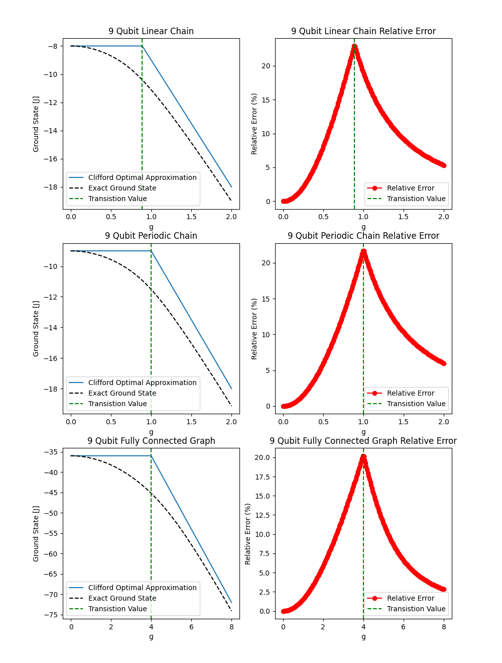
Figure 1 plots a comparison between and for the Hamiltonians obtained from and for different values of .
Figure 2 plots the relative error for with at the transition value of .
V-B Other Graphs
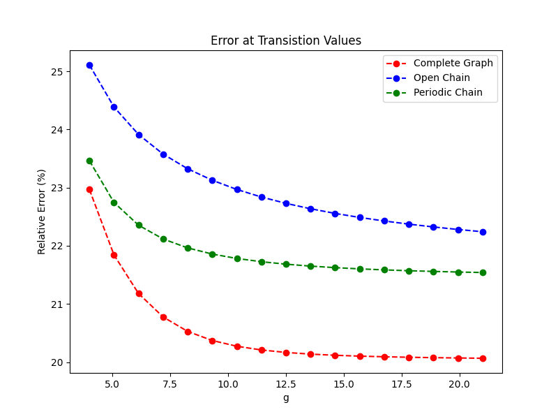
Figure 4 plots the value of versus for for a range of values.
V-C Randomized Graphs
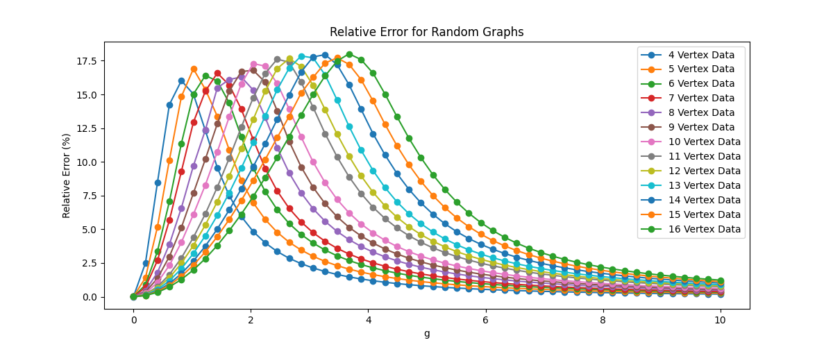
Figure 3 plots the average relative error for random graphs. For , vertex graphs were generated by randomly placing a node between every pair of vertices with probability . If the graph with no edges was obtained, this distribution was resampled.
VI Further Research
VI-A Other Hamiltonians
Here we studied a specific spin-hamiltonian. There are multiple generalizations that could have been considered.
VI-A1 Weighted Ising Hamiltonians
The most natural generalization of the Ising Hamiltonian considered here is the following
Assuming that and are both positive for all values of , we can once again tie the minimization of to the minimization of a submodular function by incorporating these terms into the cost function.
Corollary VI.1.
For a set of coefficients and ,
Where the function on the right side is a submodular function of .
An example of an application of this modified Transverse Ising Hamiltonian, which accounts for different strength spin couplings can be found in [36]. In the case where are arbitrary, more careful analysis is required to handle negative coefficients because these can cause the corresponding graph theoretic function to no longer be submodular.
An interesting variation of this Hamiltonian is the version with the terms each replaced with . Such Hamiltonians often arise from QUBOs [37][38][39]. These Hamiltonians are generally constructed so that all of their eigenvalues are Clifford, which generally implies that there is no non-NP-hard algorithm to find the optimal Clifford State for these Hamiltonians.
VI-A2 Heisenberg Hamiltonians
In the case where , we obtain the model, and in the case where we obtain the model.
Using methods similar to those in [41], it can be shown analytically that the ground state of the model and the model with is always the Clifford state regardless of the underlying graph .
Finding the optimal Clifford state for a generalized Heisenberg Hamiltonian on an arbitrary graph will likely correspond to minimizing some constrained submodular function because of the additional restrictions on which terms in the Hamiltonian can simultaneously be in a given stabilizer. Unfortunately, this means that finding the optimal Clifford state for these problems may be NP-Hard [42].
VII Conclusion
In this work we outlined an efficient method for finding the optimal Clifford ground state of a given transverse field Ising Hamiltonian on an arbitrary graph. Our numerical estimates suggest that these optimal Clifford ground states are generally fairly accurate (with errors always less than ), suggesting that CAFQA-inspired approaches to VQE problems are useful initialization techniques for these Hamiltonians.
Acknowledgement
This work is funded in part by EPiQC, an NSF Expedition in Computing, under award CCF-1730449; in part by STAQ under award NSF Phy-1818914; in part by NSF award 2110860; in part by the US Department of Energy Office of Advanced Scientific Computing Research, Accelerated Research for Quantum Computing Program; and in part by the NSF Quantum Leap Challenge Institute for Hybrid Quantum Architectures and Networks (NSF Award 2016136) and in part based upon work supported by the U.S. Department of Energy, Office of Science, National Quantum Information Science Research Centers. This research used resources of the Oak Ridge Leadership Computing Facility, which is a DOE Office of Science User Facility supported under Contract DE-AC05-00OR22725.
Appendix A Graph List
The following graphs are used throughout for computations. Notice every graph here is connected.
A-A Linear Chains
The -vertex open linear chains, , with will be defined as the graphs with nodes and only edges from to for . Figure 5 shows the first open linear chains.
The -vertex periodic linear chains, , with will be defined as with the additional edge from to . The first periodic chains are drawn in Figure 6.
A-B Fully Connected Graphs
The fully connected graph with with will be defined as the graph with vertices and an edge between every pair of vertices. Figure 7 shows the first fully connected graphs.
A-C Miscellaneous Graphs
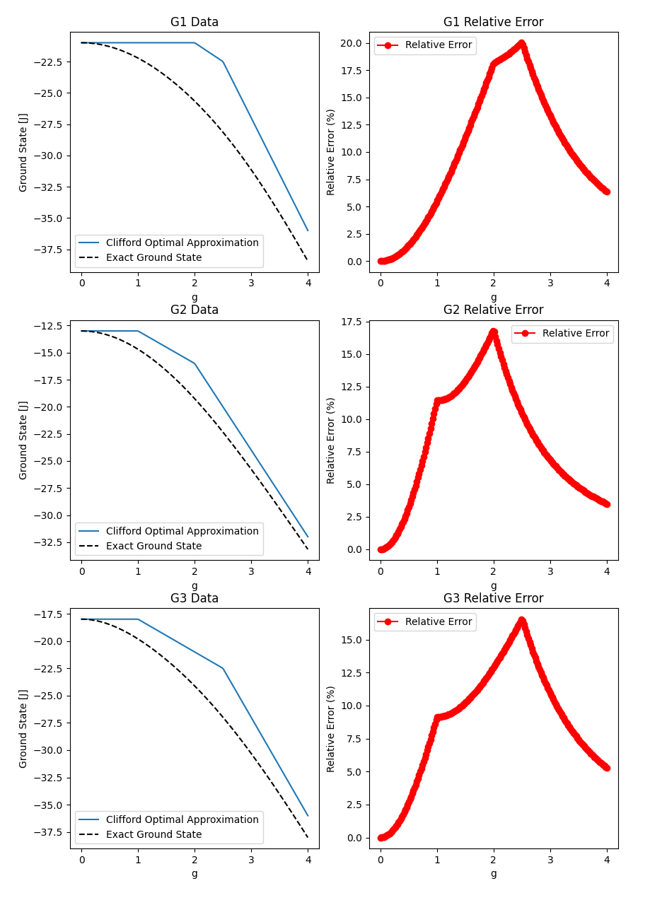
The following graphs (Figure 8) are designed to have subgraphs which are more dense than the entire graph, and thus are all not two-segmented.
These graphs will be referred as and .
Appendix B Overview of relevant algorithms
In this appendix we provide a brief overview of the relevant algorithms used in this paper. All relevant code can be found at [43].
B-A Edge Functions (DkS)
The densest k-subgraph (DkS) problem can be defined as the problem of finding the vertex set with for fixed such that is maximized. This algorithm is known to be NP-hard [44].
Clearly, computing for is equivalent to solving DkS for , meaning that computing all of the values for is an NP-hard problem.
Currently, the best known approximate algorithm for DkS was introduced in [45], and computes an approximation in .
Although edge functions are useful theoretical tools, we generally don’t need to consider specific values of when searching for the optimal Clifford state, meaning we can avoid this NP-Hard problem.
B-B Two-Segmented Testing (DSP)
The densest subgraph problem (DSP) can be defined as the problem of finding the vertex set such that is maximized. It is well known that the Densest Subgraph Problem can be solved in polynomial time [44].
One solution method uses a linear programming problem in variables, which was introduced in [46]. Another polynomial time solution was introduced in [47] and uses maximum-flow computations.
Starting with an arbitrary graph , we can always run a solution to DSP on it, and if the obtained vertex set satisfies , we immediately know that must be two segmented.
B-C Submodular Minimization
The most important algorithm used here is the algorithm to minimize the function
The following corollary immediately follows from the definition ,
Corollary B.1.
For any sets ,
Functions which satisfy corollary B.1 are called submodular functions. A comprehensive overview of submodular functions can be found in [48].
One of the most important properties of submodular functions is that they can always be minimized in polynomial time. The first algorithm to do so was introduced in [49] and [50], but this algorithm is seemingly too slow for practical applications. Another independent algorithm was introduced in [51], which uses an algorithm to minimize the norm of a point in a polyhedra introduced in [52] and theory developed in [53]. An approximation for the performance of this algorithm was obtained in [26], which provided a pseudopoynomial bound on the runtime of this algorithm.
References
- [1] G. S. Ravi, P. Gokhale, Y. Ding, W. M. Kirby, K. N. Smith, J. M. Baker, P. J. Love, H. Hoffmann, K. R. Brown, and F. T. Chong, “Cafqa: A classical simulation bootstrap for variational quantum algorithms,” 2022.
- [2] P. W. Shor, “Polynomial-time algorithms for prime factorization and discrete logarithms on a quantum computer,” SIAM Journal on Computing, vol. 26, no. 5, p. 1484–1509, Oct 1997. [Online]. Available: http://dx.doi.org/10.1137/S0097539795293172
- [3] A. Kandala, A. Mezzacapo, K. Temme, M. Takita, M. Brink, J. M. Chow, and J. M. Gambetta, “Hardware-efficient variational quantum eigensolver for small molecules and quantum magnets,” Nature, vol. 549, no. 7671, pp. 242–246, 2017.
- [4] N. Moll, P. Barkoutsos, L. S. Bishop, J. M. Chow, A. Cross, D. J. Egger, S. Filipp, A. Fuhrer, J. M. Gambetta, M. Ganzhorn et al., “Quantum optimization using variational algorithms on near-term quantum devices,” Quantum Science and Technology, vol. 3, no. 3, p. 030503, 2018.
- [5] J. Biamonte, P. Wittek, N. Pancotti, P. Rebentrost, N. Wiebe, and S. Lloyd, “Quantum machine learning,” Nature, vol. 549, no. 7671, pp. 195–202, 2017.
- [6] J. Preskill, “Quantum computing in the nisq era and beyond,” Quantum, vol. 2, p. 79, 2018.
- [7] L. K. Grover, “A fast quantum mechanical algorithm for database search,” in ANNUAL ACM SYMPOSIUM ON THEORY OF COMPUTING. ACM, 1996, pp. 212–219.
- [8] J. O’Gorman and E. T. Campbell, “Quantum computation with realistic magic-state factories,” Physical Review A, vol. 95, no. 3, Mar 2017. [Online]. Available: http://dx.doi.org/10.1103/PhysRevA.95.032338
- [9] P. Czarnik, A. Arrasmith, P. J. Coles, and L. Cincio, “Error mitigation with clifford quantum-circuit data,” 2020.
- [10] E. Rosenberg, P. Ginsparg, and P. L. McMahon, “Experimental error mitigation using linear rescaling for variational quantum eigensolving with up to 20 qubits,” Quantum Science and Technology, Nov 2021. [Online]. Available: http://dx.doi.org/10.1088/2058-9565/ac3b37
- [11] G. S. Barron and C. J. Wood, “Measurement error mitigation for variational quantum algorithms,” 2020.
- [12] L. Botelho, A. Glos, A. Kundu, J. A. Miszczak, Özlem Salehi, and Z. Zimborás, “Error mitigation for variational quantum algorithms through mid-circuit measurements,” 2021.
- [13] S. Wang, P. Czarnik, A. Arrasmith, M. Cerezo, L. Cincio, and P. J. Coles, “Can error mitigation improve trainability of noisy variational quantum algorithms?” 2021.
- [14] K. Temme, S. Bravyi, and J. M. Gambetta, “Error mitigation for short-depth quantum circuits,” Physical review letters, vol. 119, no. 18, p. 180509, 2017.
- [15] Y. Li and S. C. Benjamin, “Efficient variational quantum simulator incorporating active error minimization,” Phys. Rev. X, vol. 7, p. 021050, Jun 2017. [Online]. Available: https://link.aps.org/doi/10.1103/PhysRevX.7.021050
- [16] T. Giurgica-Tiron, Y. Hindy, R. LaRose, A. Mari, and W. J. Zeng, “Digital zero noise extrapolation for quantum error mitigation,” in 2020 IEEE International Conference on Quantum Computing and Engineering (QCE). IEEE, 2020, pp. 306–316.
- [17] G. S. Ravi, K. N. Smith, P. Gokhale, A. Mari, N. Earnest, A. Javadi-Abhari, and F. T. Chong, “Vaqem: A variational approach to quantum error mitigation,” 2021.
- [18] W. Lavrijsen, A. Tudor, J. Müller, C. Iancu, and W. de Jong, “Classical optimizers for noisy intermediate-scale quantum devices,” in 2020 IEEE International Conference on Quantum Computing and Engineering (QCE), 2020, pp. 267–277.
- [19] W. Tang, T. Tomesh, M. Suchara, J. Larson, and M. Martonosi, “Cutqc: using small quantum computers for large quantum circuit evaluations,” Proceedings of the 26th ACM International Conference on Architectural Support for Programming Languages and Operating Systems, Apr 2021. [Online]. Available: http://dx.doi.org/10.1145/3445814.3446758
- [20] Y. Zhang, L. Cincio, C. F. Negre, P. Czarnik, P. Coles, P. M. Anisimov, S. M. Mniszewski, S. Tretiak, and P. A. Dub, “Variational quantum eigensolver with reduced circuit complexity,” arXiv preprint arXiv:2106.07619, 2021.
- [21] A. Peruzzo, J. McClean, P. Shadbolt, M.-H. Yung, X.-Q. Zhou, P. J. Love, A. Aspuru-Guzik, and J. L. O’brien, “A variational eigenvalue solver on a photonic quantum processor,” Nature communications, vol. 5, p. 4213, 2014.
- [22] J. R. McClean, J. Romero, R. Babbush, and A. Aspuru-Guzik, “The theory of variational hybrid quantum-classical algorithms,” New Journal of Physics, vol. 18, no. 2, p. 023023, 2016.
- [23] J. R. McClean, S. Boixo, V. N. Smelyanskiy, R. Babbush, and H. Neven, “Barren plateaus in quantum neural network training landscapes,” Nature Communications, vol. 9, no. 1, Nov 2018. [Online]. Available: http://dx.doi.org/10.1038/s41467-018-07090-4
- [24] S. Wang, E. Fontana, M. Cerezo, K. Sharma, A. Sone, L. Cincio, and P. J. Coles, “Noise-induced barren plateaus in variational quantum algorithms,” arXiv preprint arXiv:2007.14384, 2020.
- [25] J. Romero, R. Babbush, J. R. McClean, C. Hempel, P. Love, and A. Aspuru-Guzik, “Strategies for quantum computing molecular energies using the unitary coupled cluster ansatz,” 2018.
- [26] D. Chakrabarty, P. Jain, and P. Kothari, “Provable submodular minimization using wolfe’s algorithm,” 2014.
- [27] J. Tilly, H. Chen, S. Cao, D. Picozzi, K. Setia, Y. Li, E. Grant, L. Wossnig, I. Rungger, G. H. Booth, and J. Tennyson, “The variational quantum eigensolver: A review of methods and best practices,” Physics Reports, vol. 986, pp. 1–128, nov 2022. [Online]. Available: https://doi.org/10.1016%2Fj.physrep.2022.08.003
- [28] Y. Du, Z. Tu, X. Yuan, and D. Tao, “Efficient measure for the expressivity of variational quantum algorithms,” Physical Review Letters, vol. 128, no. 8, feb 2022. [Online]. Available: https://doi.org/10.1103%2Fphysrevlett.128.080506
- [29] S. Aaronson and D. Gottesman, “Improved simulation of stabilizer circuits,” Physical Review A, vol. 70, no. 5, nov 2004. [Online]. Available: https://doi.org/10.1103%2Fphysreva.70.052328
- [30] D. Gottesman, “The heisenberg representation of quantum computers,” arXiv preprint quant-ph/9807006, 1998.
- [31] R. J. Wilson, Introduction to Graph Theory, 4th ed. Addison-Wesley Logman Limited, 1996.
- [32] R. Scheffler, “Graph search trees and their leaves,” 2023.
- [33] G. B. Mbeng, A. Russomanno, and G. E. Santoro, “The quantum ising chain for beginners,” 2020.
- [34] G. Grimmett, Probability on Graphs, 2nd ed. Cambridge University Press, 2018.
- [35] J. Strecka and M. Jascur, “A brief account of the ising and ising-like models: Mean-field, effective-field and exact results,” 2015.
- [36] M. P. Kaicher, D. Vodola, and S. B. Jäger, “Mean-field treatment of the long-range transverse field ising model with fermionic gaussian states,” Physical Review B, vol. 107, no. 16, apr 2023. [Online]. Available: https://doi.org/10.1103%2Fphysrevb.107.165144
- [37] E. Farhi, J. Goldstone, and S. Gutmann, “A quantum approximate optimization algorithm,” 2014.
- [38] K. Blekos, D. Brand, A. Ceschini, C.-H. Chou, R.-H. Li, K. Pandya, and A. Summer, “A review on quantum approximate optimization algorithm and its variants,” 2023.
- [39] J. Nüßlein, T. Gabor, C. Linnhoff-Popien, and S. Feld, “Algorithmic QUBO formulations for -SAT and hamiltonian cycles,” in Proceedings of the Genetic and Evolutionary Computation Conference Companion. ACM, jul 2022. [Online]. Available: https://doi.org/10.1145%2F3520304.3533952
- [40] B. J. Powell, “An introduction to effective low-energy hamiltonians in condensed matter physics and chemistry,” 2010.
- [41] M. V. Rakov and M. Weyrauch, “Spin-1/2 xxz heisenberg chain in a longitudinal magnetic field,” Physical Review B, vol. 100, no. 13, oct 2019. [Online]. Available: https://doi.org/10.1103%2Fphysrevb.100.134434
- [42] K. Nagano, Y. Kawahara, and K. Aihara, “Size-constrained submodular minimization through minimum norm base,” in Proceedings of the 28th International Conference on International Conference on Machine Learning, ser. ICML’11. Madison, WI, USA: Omnipress, 2011, p. 977–984.
- [43] B. Bhattacharyya, “OptimalCliffordIsing.” [Online]. Available: https://github.com/BBhattacharyya1729/OptimalCliffordIsing
- [44] T. Lanciano, A. Miyauchi, A. Fazzone, and F. Bonchi, “A survey on the densest subgraph problem and its variants,” 2023.
- [45] A. Bhaskara, M. Charikar, E. Chlamtac, U. Feige, and A. Vijayaraghavan, “Detecting high log-densities – an approximation for densest -subgraph,” 2010.
- [46] M. Charikar, “Greedy approximation algorithms for finding dense components in a graph,” in Proceedings of the Third International Workshop on Approximation Algorithms for Combinatorial Optimization, ser. APPROX ’00. Berlin, Heidelberg: Springer-Verlag, 2000, p. 84–95.
- [47] A. V. Goldberg, “Finding a maximum density subgraph,” EECS Department, University of California, Berkeley, Tech. Rep. UCB/CSD-84-171, 1984. [Online]. Available: http://www2.eecs.berkeley.edu/Pubs/TechRpts/1984/5956.html
- [48] S. Fujishige, Submodular Functions and Optimization, 2nd ed. Elsevier Science, 2005.
- [49] S. Iwata, L. Fleischer, and S. Fujishige, “A combinatorial, strongly polynomial-time algorithm for minimizing submodular functions,” 2000.
- [50] A. Schrijver, “A combinatorial algorithm minimizing submodular functions in strongly polynomial time,” Journal of Combinatorial Theory, Series B, vol. 80, no. 2, pp. 346–355, 2000. [Online]. Available: https://www.sciencedirect.com/science/article/pii/S0095895600919890
- [51] S. Fujishige and S. Isotani, “A submodular function minimization algorithm based on the minimum-norm base,” Pacific Journal of Optimization, vol. 7, 04 2009.
- [52] P. Wolfe, “Finding the nearest point in a polytope,” Mathematical Programming, vol. 11, pp. 128–149, 1976. [Online]. Available: https://api.semanticscholar.org/CorpusID:17825447
- [53] J. Edmonds, Submodular Functions, Matroids, and Certain Polyhedra. Berlin, Heidelberg: Springer-Verlag, 2003, p. 11–26.