Optimal Control of Short-Time Attractors in Active Fluid Flows
Abstract
Objective Eulerian Coherent Structures (OECSs) and instantaneous Lyapunov exponents (iLEs) govern short-term material transport in fluid flows as Lagrangian Coherent Structures and the Finite-Time Lyapunov Exponent do over longer times. Attracting OECSs and iLEs reveal short-time attractors and are computable from the Eulerian rate-of-strain tensor. Here we devise an optimal control strategy to create short-time attractors in viscosity-dominated active fluids. By modulating the active stress intensity, our framework achieves a target profile of the minimum eigenvalue of the rate-of-strain tensor, controlling the location and shape of short-time attractors. We use numerical simulations to show that our optimal control strategy effectively achieves desired short-time attractors while rejecting disturbances. Combining optimal control and recent advances on coherent structures, our work offers a new perspective to steer material transport in unsteady flows, with applications in synthetic active nematics and multicellular systems.
Large-scale coherent dynamics where global collective behaviors arise from local interactions, individual anisotropies and activity are ubiquitous. Bird flocks, bacterial swarms or ensembles of cells exhibit macroscopic patterns whose length scale is orders of magnitude larger than the individual size [Toner1995, Vicsek2012, RevModPhys.85.1143, kruse2004asters, ballerini2008interaction, zhang2010collective, bricard2013emergence, dombrowski2004self, copenhagen2021topological, meacock2021bacteria, friedl2009collective, ladoux2017mechanobiology, Doostmohammadi2018, serra2020dynamic]. The macroscopic dynamics of these systems of active individuals –or active matter– exhibit nonstandard physical properties such as self-organization, symmetry breaking and non-reciprocity [ramaswamy2017active, Marchetti2013, toner2005hydrodynamics, Fruchart2021, bowick2022symmetry, shankar2022topological]. There are several descriptions of active matter systems [shaebani2020computational], including agent-based models, coarse-grained continuum models, and data-driven models [joshi2022data]. Here we focus on hydrodynamic models, which predict the macroscopic behavior of the system from a small set of parameters and take the form of Partial Differential Equations (PDEs) describing quantities such as velocity, density and nematic tensor.
Besides studying the emergent properties of active matter, it is natural to ask how one can control such systems to steer their global dynamics. The main possibilities rely on distributed or boundary control techniques [MQS]. Experimentally, [ross2019controlling] generated desired persistent fluid flows by regulating light patterns on a mixture of optogenetically modified motor proteins and microtubule filaments. Also controlling light, [lemma2022spatiotemporal] achieved spatiotemporal patterning of extensile active stresses in microtubule-based active fluids. By controlling an external electric field affecting cellular signaling networks, [cohen2014galvanotactic] steered the collective motion of MDCK-II epithelial cells. From a theoretical perspective, [shankar2022spatiotemporal] propose a new framework to steer topological defects –the localized singularities in the orientation of the active building blocks [RevModPhys.85.1143]– by controlling activity stress patterns. [norton2020optimal] devised an Optimal Control Problem (OCP) to achieve a target nematic director field by controlling either an applied vorticity field in the nematic tensor dynamics or the active stress magnitude in the velocity dynamics. Alternative control strategies use surface anchoring at the boundaries and substrate drag to rectify the coherent flow of an active polar fluid in a 2D channel [boundaryControlGulati2022].
Existing theoretical methods target a desired configuration of the nematic director field, topological defects or fluid velocities. While defects’ dynamics drive large-scale chaotic flow [Giomi2015, PhysRevX.9.041047, Tan2019], they may not be enough to predict spatiotemporal material transport. For instance, [serra2021defect] shows in experimental and numerical active nematics that the director field alone cannot predict if different domain regions will mix over a desired time interval or remain separated by a transport barrier, as well as predict where transport barriers are. In fact, even the knowledge of the velocity field and typical streamline or vorticity plots are sub-optimal to studying material transport in unsteady flows, as shown in experimental and simulated velocities [LCSHallerAnnRev2015, serra2016objective, serra2020SR] \textcolorblackand Figure 1.
A natural framework to quantify material transport is the concept of Coherent Structures (CSs), see e.g. [LCSHallerAnnRev2015, SerraHaller2015, hadjighasem2017critical], which serve as the robust frame-invariant skeletons shaping complex trajectory patterns. CSs include Lagrangian Coherent Structures (LCSs)[LCSHallerAnnRev2015] which organize material transport over a finite time interval, and their short-time limits called Objective Eulerian Coherent Structures (OECSs) [SerraHaller2015, nolan2020finite]. Attractors, their domain of attraction and repellers are widespread CSs in embryonic development across species [serra2020dynamic, serra2021mechanochemical, lange2023zebrahub] and active nematics [serra2021defect]. Controlling material transport in active matter enables the modulation of spatial mixing or trapping in synthetic systems but also enhances our understanding and perhaps the ability to influence multicellular flows in embryonic development. any studies have been done regarding the control of liquid crystals and nematic fluids [liu2020optimal], [norton2020optimal], [lasarzik2019approximation]. oreover, several OCPs have been formulated to study living cells behaviour and tackle biological challenges, mainly in the field of tumors detection and treatment [leszczynski2020optimal], [lecca2021control], [schattler2015optimal], and in the scope of drug administration [martin1994optimal], [khalili2021optimal]. owadays, an extensively studied category of fluid control problems is the one related to the control of passive fluids. Some examples are given by De Los Reyes et al. [de2015optimal] and by Manzoni et al. [MQS], which aim at imposing a determined steady-state velocity profile to the fluid. Another largely investigated goal is the control of the vorticity of a fluid, which represents a highly interesting topic in some fields as mixing processes [mathew2007optimal] and vortexes control and attenuation[kim2006vorticity], [abergel1990some]. ore recently, the interest in the study of the control of active fluids raised, leading to an increase in the researches in that field. n this work, the active fluid presented by Serra et al. [serra2021mechanochemical] is considered. In particular, the fluid is a \albDescrizione precisa del tipo di fluido e dell’origine biologica. The aim is to define an optimal control strategy able to generate a short-term attractor in the fluid. To obtain it, a possible option could be to impose a reference target to the velocity field of the fluid and to minimize a cost functional associated with the difference among the actual velocity field and the reference one. Nevertheless, such an option would be the best only in case of stationary flow conditions, which is, in general, not the case. Moreover, also in case of stationary systems the short-term attractors are different from the long-term ones, and this is caused by the fact that the short-term attraction dynamics is not the asymptotic one [serra2016objective] \albqui Mattia aveva fatto una speigazione abbastanza esaustiva di questa differenza utilizzadno questo suo vecchio articolo ma non ho segnato bene/ricordo tutto nel dettaglio. Thus, a much more convenient choice is to control one eigenvalue associated with the rate of strain tensor of the fluid, defined as . Indeed, the eigenvalues of the rate of strain tensor, i.e. and , rule the amplitude of the local stress inside the fluid, and the corresponding eigenvectors, and respectively, determine the directions of the stresses. Thus, minimizing the value of the smaller eigenvalue leads to the generation of a negative stress in a portion of the domain, which forces the attraction of the surrounding material. So, acting on allows to generate a negative stress field, in which the direction of maximum normal attraction is determined by .
As for the fluid, it is necessary to introduce some parameters. The first one is the active stress , which is the stress component present inside the fluid. In the work presented by Serra et al. [], this stress is generated by some cables of active myosin inside the fluid. These cables are also characterized by their orientation , which highly affects the way in which acts on the fluid. Then, is the ratio of the shear to the bulk modulus of the fluid and accounts for its compressibility. Alongside with , is the ratio of the isotropic to anisotropic active stress and it is used to account for the effect of the active stress on the compressibility: indeed, is used to introduce additional compressibility to the regions of the domain in which there is a higher concentration of active stress.
Here, we consider the OCP of a simplified version of the compressible active fluid introduced in [serra2021mechanochemical, chuai2023reconstruction] to describe multi-cellular movements in vertebrate gastrulation. In the hydrodynamic approximation, the system’s states are described by PDEs that couple the multicellular fluid velocity , the orientational dynamics , which dictates the anisotropy of the active stresses, and which describes the active stress intensity. We seek to control the location and shape of short-time attractors marking regions of material accumulation.
1 Material Transport
Long-term material transport is a fundamentally Lagrangian phenomenon, originally studied by keeping track of the longer-term redistribution of individual tracers released in the flow. In that setting, the Finite Time Lyapunov Exponent (FTLE) and Lagrangian coherent structures (LCSs) have been efficient predictors of tracer behavior see e.g. [haller2015lagrangian, shadden2005definition, hadjighasem2017critical, serra2017uncovering, serra2020dynamic, serra2021defect]. An alternative to Lagrangian approaches is to find their instantaneous limits purely from Eulerian observations, thereby avoiding the pitfalls of trajectory integration, while predicting short-term material transport. Additionally, LCSs are generally impractical to control – no literature exists – because they are defined as nonlinear functions of fluid trajectories, which are themselves integrals of the Eulerian velocity .
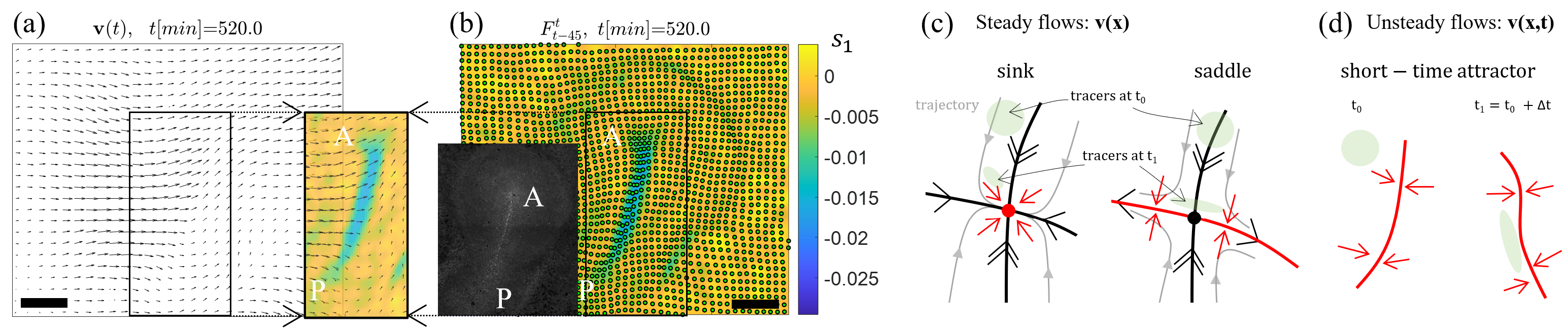
Short-time attractors – originally defined as Attracting OECSs [serra2016objective] – govern material transport in fluid flows over short-times, revealing critical information in challenging problems such as search and rescue operations at sea [serra2020search] and oil-spill containment [duran2021horizontal]. A simpler, more controllable alternative to attracting OECSs for locating short-time attractors is the instantaneous Lyapunov Exponent (iLE)[Nolan2020], defined as the instantaneous limit of the well known FTLE. The iLE locates short-time attractors as trenches – or negative regions – of the smallest eigenvalue of the rate-of-strain tensor of the fluid velocity . \textcolorblackFor example, Figs.1a-b show short-term attractors marked by trenches of (scalar field) in an experimental velocity field (black vector field) describing the motion of thousands of cells during chick gastrulation [Rozbicki2015]. A strong trench of marks a short-term attractor along the anterior-posterior (AP) axis corresponding to the forming primitive streak [serra2020dynamic] (panel b), while remaining not identifiable from the inspection of the corresponding velocity field (panel a and its inset). Similar results hold in different flows (see e.g., Fig. 1 of [serra2016objective] and Figs. 4-5 of [serra2020search]). To confirm the effect of short-term attractors, panel b shows that tracers (green dots) released from a uniform grid of initial conditions and advected by for a short time accumulate on the trench.
blackClassical asymptotic attracting structures (Fig. 1c) include sink-type fixed points (red dot) and the unstable manifold (red curve) of saddle-type fixed points of steady velocity fields. These structures, however, cannot move or deform in time and influence material transport only for steady velocity fields. \textcolorblackAs shown in Figs.1a-b, inspection and control of the velocity field is sub-optimal to create material traps in general unsteady flows. First, because the velocity field and its streamlines are not objective, i.e., they depend on the choice of reference frame used to describe motion (see also SM Section 6 and Figs. S1-S2). By contrast, the location of material accumulation is frame invariant [haller2015lagrangian, serra2016objective], as any quantification of the material response of a deforming continuum must be according to a fundamental axiom of mechanics [gurt]. Second, it might be an unnecessarily strong requirement, or uncompliant with boundary conditions, to prescribe directly. \textcolorblackOn the other hand, short-time attractors (Figs. 1b,d) are frame invariant, can move and deform, and apply to general unsteady flows. Here we devise an optimal control framework that uses the active stress intensity as the control input to achieve a target short-time attractor, defined by a desired distribution of or iLE, in active viscous flows.
2 Active Fluid Model
We adopt a simplified version of the mechanochemical model developed in [serra2021mechanochemical] consisting of an active stokes flow characterized by the passive viscous stress and active stress , where is the deviatoric rate-of-strain tensor, characterizes the orientation of active elements , denotes the intensity of active stress and the identity tensor. To account for flow compressibility, we use a simple continuity equation where positive isotropic viscous stress (), and isotropic contractile-type () active stress contribute to negative flow divergence via the bulk viscosity and a nondimensional parameter . Biologically, modulates the cell propensity to ingress into the third dimension given active isotropic apical contraction. The resulting system of PDEs in nondimensional form [serra2021mechanochemical] is
where is a second nondimensional parameter characterizing the ratio of the shear to bulk viscosity, and . The first two terms in the force balance describe passive forces due to shear and compressibility, while the active forces arise from spatial variations of and . To set up our optimal control problem, we consider a simplified dynamics where the orientation of active elements is time-independent and prescribed, while the active stress intensity is the control input.
s a consequence, the state equation has the same structure found in linear elasticity theory i.e. Navier-Cauchy equations which, however, describe the displacement dynamics.
3 Results
To control short-time attractors, the OCP involves steering the minimum eigenvalue of the rate of strain tensor towards a target function while minimizing the overall control effort and its gradient:
| (1) |
where represents a scalar target for the minimum eigenvalue of the rate-of-strain tensor of , and is a disturbance on the state dynamics.
Following a Lagrangian variational approach, we derive a system of first-order necessary optimality conditions for the OCP problem. We note that is nonlinear and nonquadratic due to the relation . Consequently, sufficiency is not guaranteed, as typical in nonconvex problems. We define the Lagrangian as
where is the adjoint function, and obtain the strong form of the optimality conditions by imposing the first variations of the Lagrangian to be zero for all allowed variations of the state, adjoint and control functions. We provide the complete derivation in the SM Sections 2-4, and summarize here the necessary conditions as a coupled system of PDEs. The optimal pair for the OCP \eqrefOCP_l should satisfy the following system of first-order necessary conditions
| (2) |
where is the eigenvector function associated to . We note that \eqrefnc requires an iterative method due to the nonlinear relationship between and the forcing term of the adjoint equation involving and .
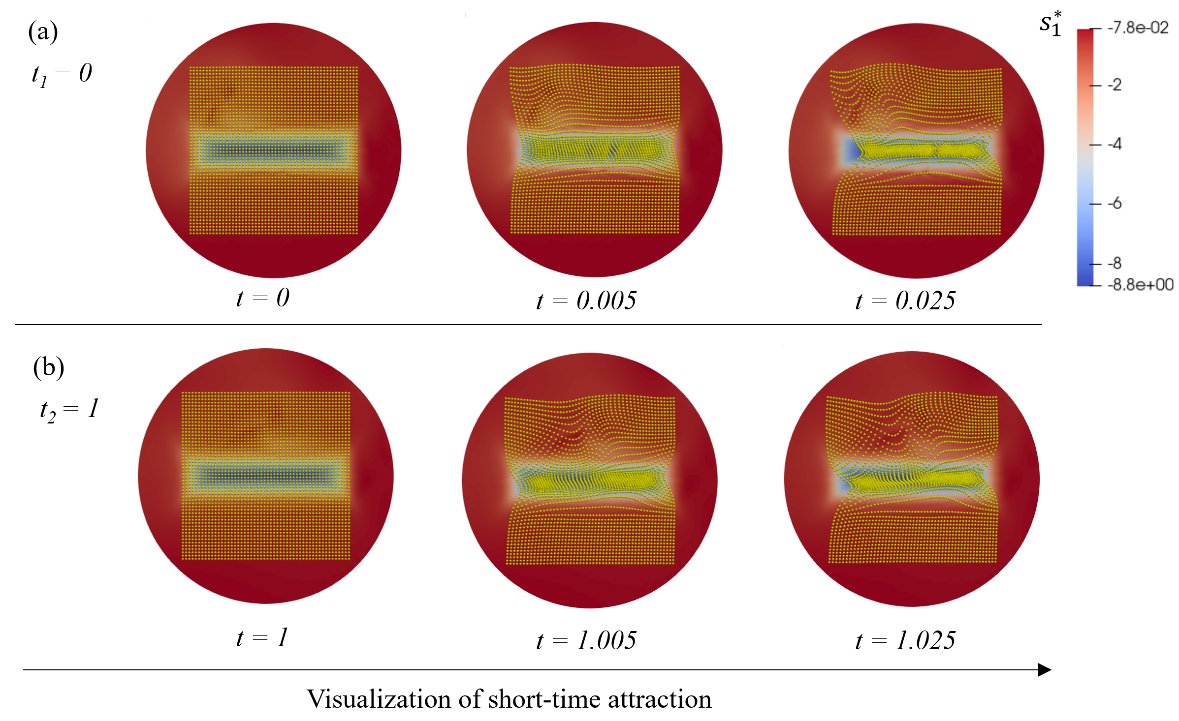
We numerically solve \eqrefnc using the Finite Element Method (FEM) and a gradient-based algorithm (SM Sec. 5). We consider a circular domain with zero velocity boundary conditions and note that our algorithm applies to arbitrary-shaped domains. We set the target shape as a scaled indicator function of a rectangle so that the target value is inside the rectangle and zero elsewhere. We set the cable orientation to a constant value from the x-axis and choose the control weighting parameter and the nondimensional model parameters . modulates the overall fluid compressibility while high induces high negative divergence in regions with higher [serra2021mechanochemical]. We select the space-time varying disturbance force as \textcolorblack, where , , and set the intensity , and standard deviation . Figure 2 shows the resulting optimal along with a grid of particles advected over short times for two different initialization times. Figura 4:
| (3) |
| (4) |
| (5) |
Figura 3:
| (6) |
| (7) |
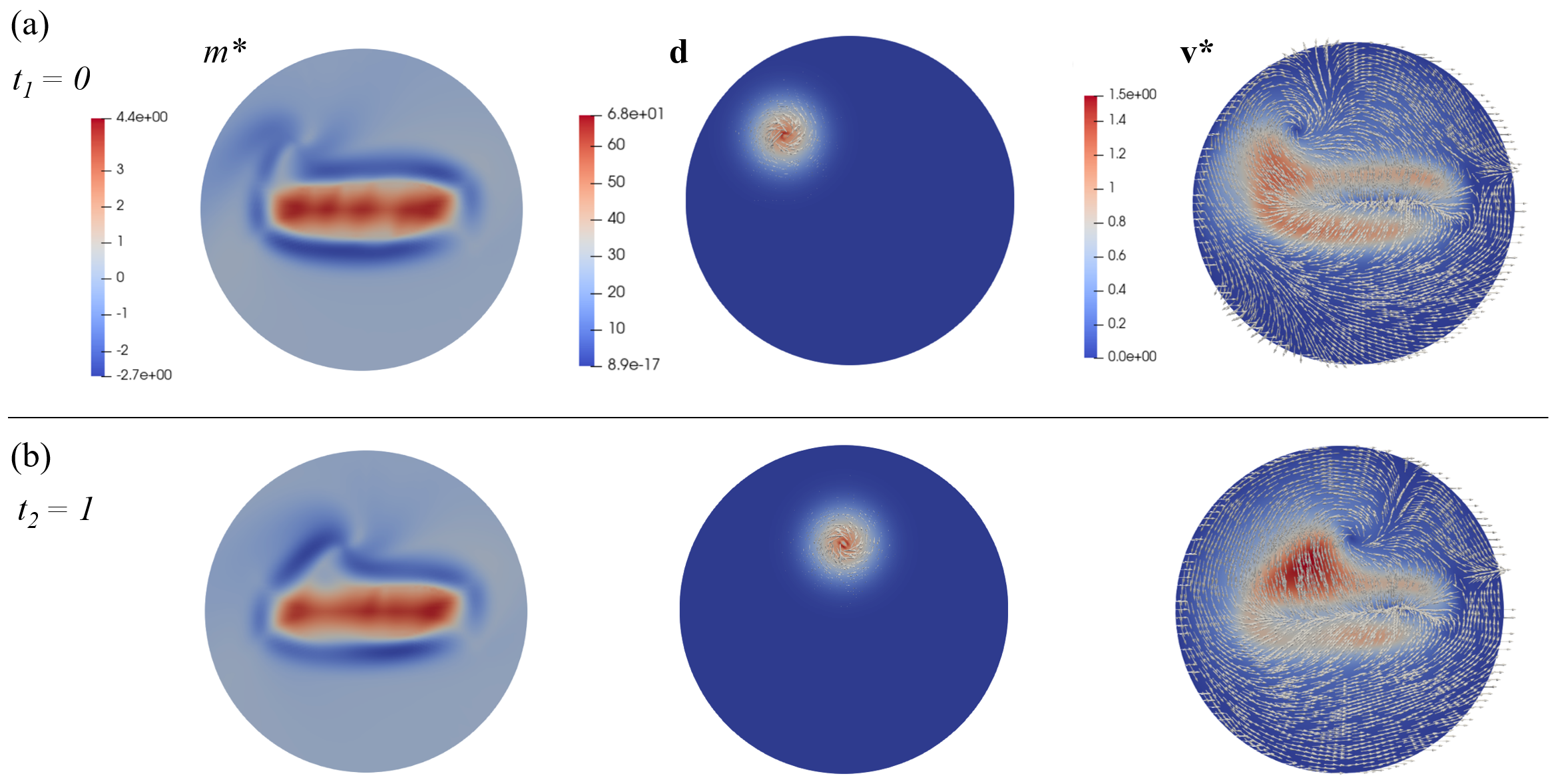
Figure 3 shows the optimal state-control pair and its associated disturbance forcing . The control acts through , and therefore both and contribute to the state dynamics. This is why the control generates sharp gradients to track the target eigenvalue accurately. Furthermore, the control field rejects the disturbance by generating a vortex-shaped counteracting effect. Overall the disturbance strongly influences the optimal velocity. Figure 4 shows the interplay between the control weight , the disturbance and the accuracy of the tracking objective that is key to generating a short-time attractor. As in the earlier figures, each row (a-b) corresponds to a different time ().
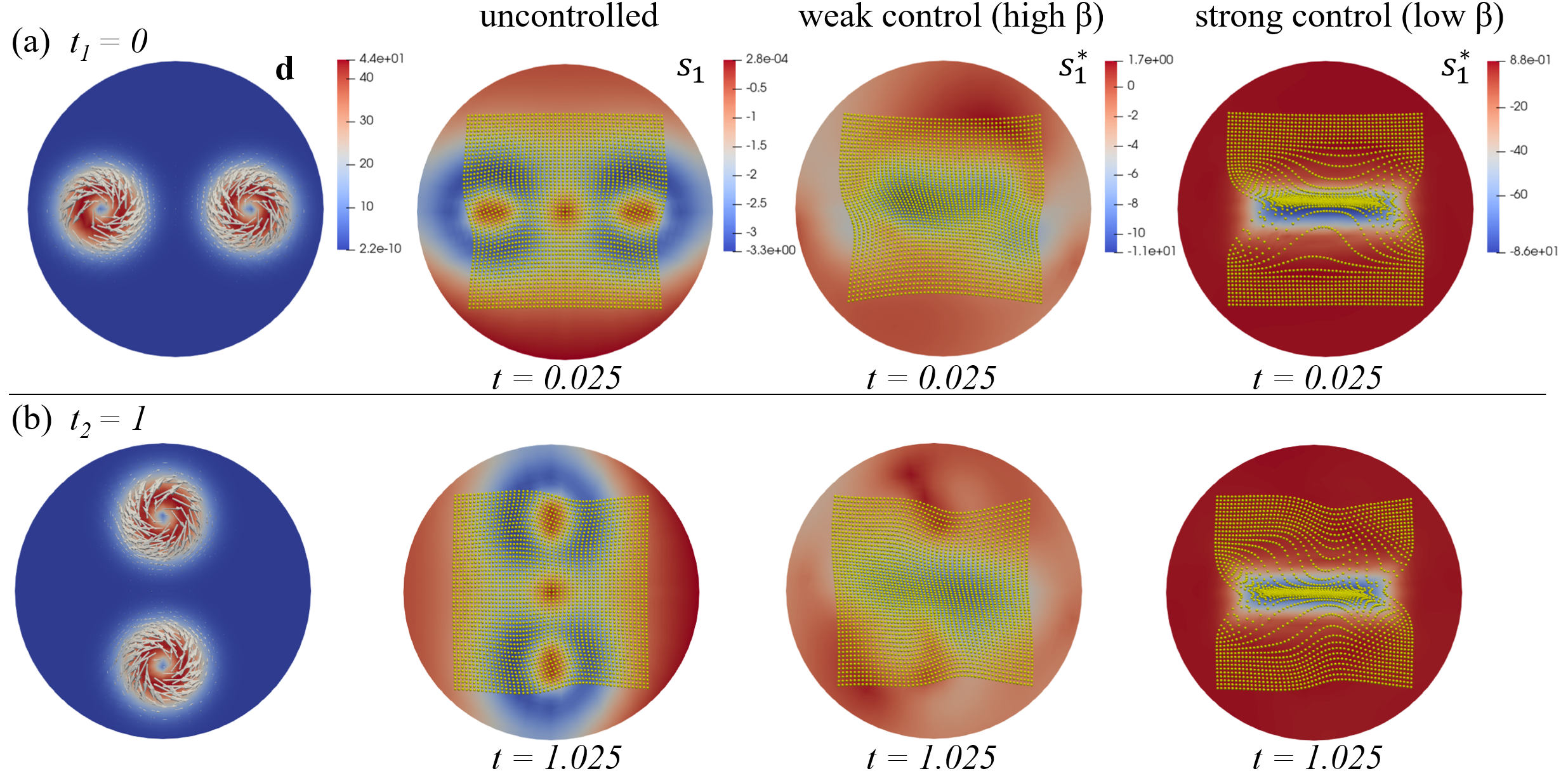
To present an additional test case, we select a different disturbance compared to Figs. 2-3, generating two vortex-shaped force-field streamlines (Figure 4, first column) using the same functional form in the previous test case. The target eigenvalue is the same as in Figs. 2-3. The uncontrolled dynamics () does not generate attraction, as shown by short-term advected particles (yellow dots) and the field in Figure 4, second column. A high (or weak control) steers the eigenvalue towards the target, but its effect is too mild to generate short-time attraction (Figure 4, third column). Indeed, a higher control weight would result in a lower relevance of the tracking term in the cost function and hence poor tracking performances. Figure 4 fourth column shows the results for a low (or strong control), as in Figure 2, resulting in the desired short-time attractor that serves as a material trap while rejecting disturbances. Different rows (a-b) show the same results for two different initialization times as in Figs. 2-3.
figure
![[Uncaptioned image]](Figures/sim_1.png) Optimal fields for , , and where the target is a combination of radial basis functions with zero mean. The broken symmetry in the top fields is due to the directionality imposed by .
Optimal fields for , , and where the target is a combination of radial basis functions with zero mean. The broken symmetry in the top fields is due to the directionality imposed by .
figure
![[Uncaptioned image]](Figures/param_comparison.png) Optimal state and control norm as a function of the control weighting and the parameter . In the sweep while in the sweep is set at . \crlCapire il minimo di norma di controllo per
Optimal state and control norm as a function of the control weighting and the parameter . In the sweep while in the sweep is set at . \crlCapire il minimo di norma di controllo per
4 Conclusion
By combining recent advances in coherent structures from nonlinear dynamics, control theory and active matter, we formulated, analyzed and numerically solved an optimal control problem that generates material short-time attractors at desired locations while rejecting disturbances. We used a simplified version of model [serra2021mechanochemical] describing a compressible, viscosity-dominated, active fluid representing a planar multicellular flow, and used the active stress intensity as the control input. We identify short-time attractors as the smallest instantaneous Lyapunov exponent [Nolan2020], the instantaneous limit of the well-known FTLE, which is computable from the smallest eigenvalue of the rate of strain tensor of the flow velocity.
Short-time attractors are frame invariant and predict the correct location of material attraction, which may be undetected from the inspection of the frame-dependent velocity field (Fig. 1, [serra2016objective, serra2020search]). Using the same framework, one can control the position of material repellers, which, together with attractors, shape complex motion in synthetic active matter [serra2021defect] and embryo morphogenesis across species [serra2020dynamic, lange2023zebrahub]. Controlling attractors and repellers offers a new, robust, and frame-invariant perspective to steer motion in synthetic and natural active matter. It will enable the creation of material traps for medical applications as well as enhance our understanding and the possibility of manipulating multicellular flows in morphogenesis. For example, it will shed light on how myosin activity (active stress intensity) generates the required motion that compartmentalizes the embryo, segregating distinct cell types (repellers) and steering specific cells to precise locations (attractors). In future work, we plan to consider the explicit orientational dynamics of the active stress anisotropy, the effect of inertial forces, and the control of Lagrangian Coherent Structures that shape fluid motion over longer time scales.