Also at ]Nano Life Science Institute, Kanazawa University, Kanazawa 920-1192, JapanAlso at ]Institute of Industrial Science, The University of Tokyo, Tokyo 153-8505, Japan Also at ]Universal Biology Institute, The University of Tokyo, Tokyo 113-8654, Japan
Optimal control of stochastic reaction networks with entropic control cost
and emergence of mode-switching strategies
Abstract
Controlling the stochastic dynamics of biological populations is a challenge that arises across various biological contexts. However, these dynamics are inherently nonlinear and involve a discrete state space, i.e., the number of molecules, cells, or organisms. Additionally, the possibility of extinction has a significant impact on both the dynamics and control strategies, particularly when the population size is small. These factors hamper the direct application of conventional control theories to biological systems. To address these challenges, we formulate the optimal control problem for stochastic population dynamics by utilizing a control cost function based on the Kullback–Leibler divergence. This approach naturally accounts for population-specific factors and simplifies the complex nonlinear Hamilton–Jacobi–Bellman equation into a linear form, facilitating efficient computation of optimal solutions. We demonstrate the effectiveness of our approach by applying it to the control of interacting random walkers, Moran processes, and SIR models, and observe the mode-switching phenomena in the control strategies. Our approach provides new opportunities for applying control theory to a wide range of biological problems.
I Introduction
Optimal control problems for a population of stochastically interacting particles arise in diverse fields of biology [1, 2]. In intracellular chemical reactions, molecules interact stochastically and nonlinearly to generate complex dynamics, whose control is essential for medical and bioengineering applications [3]. In cellular or animal populations, cells or organisms with different phenotypic and genetic traits interact and compete for survival and reproduction. Strategic control of such populations into either extinction, survival, or amplification leads to cancer therapy [4, 5, 6], stem cell culturing [7], manipulating gut microbiota [8], maintenance of immunological memory [9, 10], biodiversity conservation [11, 12, 13], and control of evolving population [14, 15] In human populations, control of epidemic outbreaks, spurred by individual interactions, poses a significant public health challenge [16, 17, 18].
All these phenomena can be effectively formulated using the theoretical framework of reaction networks (RN), making stochastic RN theory a firm foundation for devising optimal control strategies across these areas (Hereafter, we use RN to designate this class of dynamics including chemical reactions, population dynamics, and epidemic dynamics.).
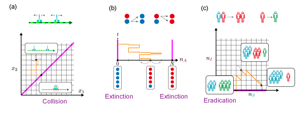
Despite its broad applicability, the optimal control of RNs remains underexplored. This oversight is largely due to the unique characteristics of stochastic RNs, which deviate from the setup of conventional optimal control for diffusion processes. The major deviations include the inherent nonlinearity of RNs, the discrete nature of state variables (representing counts of particles like molecules or organisms), and their stochastic dynamics, which are better modeled by Markov jump processes with Poissonian randomness rather than Gaussian diffusion [19, 1, 20]. Additionally, the non-negativity constraint of control parameters, i.e., kinetic rate constants, requires a natural measure for cost other than conventional quadratic ones, which presume the constraint-free Euclidian parameter space. Finally, the zero count states act as intrinsic absorbing boundaries, reaching them can dramatically alter system dynamics through the extinction of particles (Fig. 1).
These distinct properties of RNs necessitate (1) a departure from the traditional control theories based on diffusion processes, such as the Linear-Quadratic-Gaussian (LQG) model, (2) an establishment of alternative theoretical framework tailored to the unique requirements of RN optimal control, and (3) its applications to biologically relevant control problems.
In this work, we establish that all these issues can be resolved by integrating optimal control of jump processes and stochastic RN with a cost function based on relative entropy or Kullback–Leibler (KL) divergence. The optimal control with KL cost was originally proposed for diffusion processes in relation to the duality of control and inference [21, 22, 23]. We demonstrate that KL cost, as it is designed for non-negative probabilities and densities, can naturally accommodate the non-negativity constraints for both state space (particle counts) and control parameters (kinetic rate constants) of stochastic RN. Moreover, KL cost allows for the linearization of the nonlinear Hamilton–Jacobi–Bellman (HJB) equations through the Cole-Hopf transformation. This linearization facilitates the efficient derivation of optimal solutions in a similar matter with previously identified solvable control problems [24, 25, 26].
By leveraging the sound properties of optimal control for stochastic RN with KL cost, we demonstrate the effectiveness of our theory for different biological phenomena: an optimal transport by mutually excluding molecular motors, maintenance of cellular heterogeneity in populations, and epidemic outbreak control (Fig. 1). For molecular motors, we derive analytic solutions owing to the linearization. In the maintenance of heterogeneity and epidemic outbreak control, we identify mode-switching phenomena of population control that hinge on the transition in controllability of exponentially growing populations.
All these results are obtained without directly solving nonlinear HJB equations, which are typically intractable, even numerically. Thus, our new results can substantially broaden the scope of optimal control applications in stochastic chemical reactions, population dynamics, and epidemics.
II Optimal control of stochastic reaction systems
II.1 Stochastic reaction systems
Let us consider a population of particles that evolve through stochastic events, i.e., the occurrence of reactions. Each particle is assigned one of discrete type set . The number of particles of type at time is denoted as . The number distribution completely characterize the state of the system at time . The number distribution changes when a reaction occurs. There are kinds of reactions, where is the set of reactions. Once a reaction occurs, particles are consumed and particles are produced. The net change in the number of particles is called stoichiometric coefficient and is stoichiometric vector for reaction . Thus when the reaction occurs at time , the number distribution changes from to
| (1) |
The timing of reaction events is random, which follow an inhomogeneous Poisson process with rate for reaction at time . It could vary over time and depends on the current number distribution . We write the rate of reaction as the product of the reaction rate coefficient and the propensity function :
| (2) |
When we assume the law of mass action kinetics, is a kinetic constant, and the function is given by , where is a constant parameter that describe the system size, e.g., the volume or total number of the particles in the system. We do not assume the mass action kinetics in the following so that our results become applicable to any propensity function. Instead, we presume only the situations that make the process well-defined up to time or up to exit time . For example, should be when the reaction pushes the state out of the domain, i.e., .
The stochastic reaction system defined in this way can be characterized by either the counting process representation or the Markov process representation. The counting process representation [20] is useful for characterizing the stochastic process and simplifies the derivation of KL control cost. Let denote the number of occurrences of reaction from time to . The number distribution is a linear transformation of the reaction count , i.e., for any ,
| (3) |
The probability law of is given by the Poisson processes. Using the time-change of independent unit Poisson processes , the reaction count can be written as .
The stochastic process is a Markov process on the nonnegative integer lattice . The transition rate from to is given by
| (4) |
where is the Kronecker delta. Let denote the probability of being the state at time given the initial state . Then, satisfies the Kolmogorov forward equation (chemical master equation) for any and :
| (5) |
II.2 General formulation of optimal control problems
We assume that the controller can observe the current state and adjust the reaction rate coefficients to any desired value at any time while the function remains unchanged, i.e., the controller can modulate only the speeds of reactions. We would like to find the optimal reaction rate coefficients which drive the population to take a desirable trajectory while minimizing the cost of modulating the reaction rate coefficients. Let us define the utility function as the sum of the terminal utility function and the time integral of instantaneous utility function . The control cost function is also defined as . Then, we consider the following optimization problem:
| (6) | ||||
or equivalently, the following unconstrained optimization:
| (7) |
where the expectation is taken over trajectories generated under the designated reaction rate coefficients and initial condition . A scalar is the Lagrange multiplier or a parameter to adjust the importance of the utility relative to the control cost.
We will calculate the optimal transition rate that attains the optimum of and . The standard protocol for solving the problem is to consider the value function , which is defined as the maximum of the expectation in Eq. (7) from to under the condition :
| (8) |
where and are the utility and control cost functions from time to , e.g., . The value function is equal to the terminal utility function at time , , and also provides the optimum for the original problem at time , . Thus, the transition rate attaining Eq. (8) is identical to the optimal transition rates in the original control problem.
If were analytically or numerically obtained for all and , in Eq. (6) is derived as the Legendre transformation of : (see Sec. A in the Supplementary Material 111See Supplemental Material at for the derivation of equations and detailed numerical results, which includes Refs. [59, 60, 61, 62, 63, 64]. for the derivation)
| (9) |
Furthermore, the expected utility under the optimal control can also be derived from the value function (see Sec. A of the Supplementary Material [27] for the derivation)
| (10) |
II.3 Optimal control with KL cost
To obtain the value function, we usually leverage the Hamilton–Jacobi–Bellman (HJB) equation, a differential equation that satisfies. However, solving the HJB equation is generally intractable both analytically and even numerically because it is a nonlinear differential equation on a possibly infinite domain. This difficulty is the major obstacle to optimal control in applications. To address the difficulty, we are conventionally forced to restrict or approximate the original problem to a linear quadratic Gaussian (LQG) problem, in which only the linear dynamics on continuous Euclidean space with Gaussian noise with a quadratic control cost function can be considered. However, all these restrictions of the LQG problem conflict with the essential properties of stochastic RN control, i.e., the nonlinearity of , the discreteness and nonnegativity of state , the nonnegativity of the control parameter , and Poissonian nature of stochasticity. Several studies attempted to overcome a part of these difficulties [28, 29, 30]. Nonetheless, optimal control was not practical for biological problems described by RN.
In this work, we clarify that the difficulty can be resolved by adopting the following cost function
| (11) |
where is the generalized Kullback–Leibler (KL) divergence for positive scalars :
| (12) |
The value at is defined by the limit .
The KL control cost function in Eq. (11) measures the deviation of the controlled reaction rate coefficient from its uncontrolled reaction rate coefficient . Because the control cost function is minimized at , the optimal reaction rate coefficient is equal to when , i.e., no preference on the state trajectory. If , the optimal reaction coefficient for at time is given by
| (13) |
where is the discrete gradient (see Sec. A of the Supplementary Material [27] for the derivation). As the slope of goes to infinity, for , the nonnegativity constraint over is automatically satisfied. In fact, the exponential function in Eq. (13) ensures that the optimal coefficient is non-negative.
Note that the KL control cost in Eq. (11) is weighted by the propensity function for each reaction , which makes the control cost function depend on the current state . It means that even if the reaction rate coefficient is the same, the control cost for a reaction is higher when the reaction occurs more frequently. A similar form of the control cost function has been used in quantifying the biological cost of cellular reactions [31].
For the KL cost function, the HJB equation becomes
| (14) | ||||
which is yet a nonlinear differential equation. However, by the Cole–Hopf transformation (logarithmic transformation), , the HJB equation is linearized as
| (15) | ||||
with the terminal condition .
Although it is still an ordinary differential equation on a possibly infinite domain, linearity allows us to calculate the value function efficiently. Note that the second term on the right-hand side is the backward operator (generator) , which is the adjoint of the forward operator in the chemical master Eq. (II.1). Moreover, the special form of Eq. (15) allows us to have the following probabilistic representation for :
| (16) |
which is called the Feynmann-Kac formula, cf., Appendix 1. Prop. 7.1 of [32]. Thus, the value function is given by
| (17) |
This representation enables us to compute the value function by evaluating the expectation of the utility function with respect to the uncontrolled reaction rate coefficient . For simple reaction systems, we could obtain the analytical expression of the value function as demonstrated in the following sections. Even if it is not possible, efficient Monte Carlo sampling techniques can be used to estimate the expectation. It is worth noting that this representation of the value function can be evaluated in a time-forward manner, whereas the usual optimal control problem requires the time-backward calculation of the HJB equation due to the dynamic programming principle.
The linearization of the HJB equation and efficient computation of the optimal control problems for certain control cost functions was reported by Kappen [24] for diffusion processes and by Todorov [26] for discrete-time Markov chains. As Theodorou and Todorov [33] discussed, the linearization of the HJB equation is possible if the control cost function is given by KL divergence between path measures. In this case, the optimal control problem is related to an estimation (filtering) problem. Similar mathematical properties had been found in relation to the duality of control and inference [21, 22, 23]. Similar properties for Markov jump processes are identified in recent studies [34, 35, 36] as well as one of the earliest studies by Fleming [21]. In this paper, we develop the optimal control framework for stochastic RN inspired by these previous studies. In Sec. B of the Supplementary Material [27], we elaborate on the path measure perspective and why the KL cost function in Eq. (11) works.
II.4 First exit optimal control with KL cost
We have hitherto focused on the problem with a finite and fixed terminal time . One can extend our approach to the problem with infinite time length . Since a stochastic reaction system often has absorbing states , the stochastic process inevitably reaches one of these absorbing states after some time . For example, in the birth-death processes
| (18) |
the extinction state is absorbing. The extinction events are particularly important in biological problems because the extinction of some spieces in a chemical, organismal, or human population could alter the dynamics of the system qualitatively. Thus, controlling species into either survival or extinction has many applications, as mentioned in the Introduction. Moreover, biological control problems may not always have a prescribed end time because the goal of control is usually to achieve something rather than to do something until . Thus, the first exist control is more essential than fixed-time control. Nevertheless, it has been less practiced because the first exist control is more involved technically.
We can consider the optimal control problem with such random terminal time and KL cost. The utility function is replaced with the sum of the terminal utility function defined on the absorbing states , and the instantaneous utility function defined on the non-absorbing states , i.e.,
| (19) |
Then, the value function becomes time-independent . If we assume the KL control cost, and the Cole–Hopf transformation yields
| (20) |
for , and for . Thus, the first exit optimal control problem is reduced to a linear algebraic problem. Similar results have been obtained for discrete-time Markov chains [26]. The probabilistic representations in Eqs. (16), (17) are also applicable.
If there are no absorbing states, the terminal time and the time accumulated objective function could diverge. For such cases, the time-averaged formulation is useful:
| (21) |
Via the Cole–Hopf transformation, the optimal solution could be cast into an eigenvalue problem (see Sec. C of the Supplementary Material [27]).
II.5 Controlling a random walker
We demonstrate the effectiveness of our method by applying it to several control problems. The first example is the jump processes on discrete states . We consider particles walking on a directed graph , where the set of directed edges represents the allowed transitions between types . For any , implies that the particle can jump from to . The stoichiometric coefficients are given by and the kinetics is the mass action type for .
For and , the process is reduced to a simple one-dimensional random walk by a single walker. Such a process has been used as a simple model of intracellular transport of macromolecules along intracellular filaments [37]. Molecular motors such as dynein and kinesin consume energy and move in one direction. Since the step length is fixed, the position of a molecular motor on a filament can be modeled as a 1-dimensional discrete grid. For this case, we can have analytical solutions for some optimal control problems owing to the sound properties of KL control.
Consider the situation where a particle is required to reach a goal as soon as possible. The position of the particle at time is denoted as . We can formulate the situation as the following minimum exit time problem:
| (22) |
where the absorbing states are given by . Setting and , we have an equivalent maximization problem
| (23) |
Equation (17) shows that the value function is equal to the cumulant-generating function of the exit time with parameter and given by
| (24) |
Assuming the symmetric uncontrolled transition rates for all and using the analytical expression of the cumulant-generating function [38], we obtain the value function analytically:
| (25) |
where a scalar is defined as
| (26) |
The conjugate value function can be calculated for and as follows
| (27) |
where . Since the value function is linear in , we have the piecewise constant optimal transition rates:
| (28) | ||||
When , the transition rate in the positive direction is higher than the uncontrolled one , while the transition rate in the negative direction is lower than . We can also obtain the analytic solution for the standard control problem to maximize the average speed of the walker (see Sec. D of the Supplementary Material [27]).
II.6 Controlling interacting random walkers
Next, we consider the case where and . Let us consider the minimum time problem with exclusion interaction, i.e., all the particles should reach the goal as soon as possible while they are not allowed to occupy the same site. This is a model of two molecular motors moving on the same filament on which they cannot overtake (Fig. 1 (a)). Non-colliding random walks and diffusion processes have been studied persistently [39, 40, 41].
Let us denote the position of the left particle as and the right particle as , i.e., . Due to the exclusive interaction, the first particle cannot overtake the second. Thus, the particles are identifiable for all . The absorbing states are given by
| (29) |
Among the abosrbing states above, we are interested in the single state such that the particles reach the goal . We can formulate the problem as a first exit problem with the instantaneous utility , and the terminal utility
| (30) |
Assuming that each particle stops when it reaches the goal, the time-integrated instantaneous utility is given by
| (31) |
where is the first exit time of the -th particle (). Then, the value function can be calculated as
| (32) | ||||
where is the value function in Eq. (25) for a single random walker. When the first particle is close to the goal while the second particle is still away from it, , the upper bound become tight and we have
| (33) |
Using the upper bound, the conjugate value function satisfies
| (34) |
where is the conjugate value function in Eq. (27).
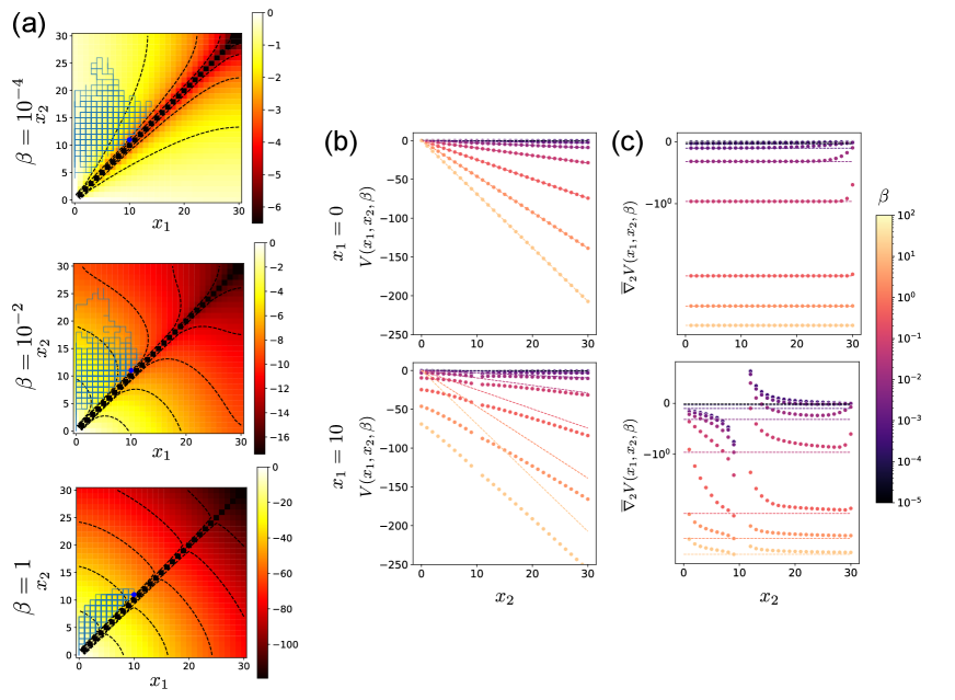
Analytical estimates are compared with numerical solutions in Fig. 2. Numerical solutions are obtained by solving the linear equation in Eq. (20) where the infinite space is truncated to the finite interval . The goal position is set to .
When the first particle has already reached the goal , the problem is equivalent to the minimum time problem for the second particle only. Then, the value function satisfies , which is consistent with Eq. (33) (Fig. 2 (b), upper panel). Then, the gradient of is constant (Fig. 2 (c), upper panel), which results in the constant optimal control.
When the first particle is at , the value as a function of has a gentle slope than to avoid collision with the first particle (Fig. 2 (b), lower panel). Especially when is small, collision avoidance is more important than early arrival. In this case, the value gradient can be positive, and the second particle moves away from the first particle, as seen in Fig. 2 (c) lower panel. On the other hand, when is large, the exit time becomes more important than the collision. Thus, the value gradient is always negative except at the collision point, i.e., at .
II.7 Controlling survival in birth and death processes
In the control of birth and death processes of cells or organisms without immigration, the extinction state is a natural absorbing state. In the context of biodiversity conservation, one has to avoid the extinction. Furthermore, a single species should not dominate the ecosystem. To address this population control problem, let us consider the following birth and death reactions involving two species and (Fig. 1 (b)):
| (35) | |||
Assume that every dying individual is replaced by a duplicated individual of either or , and that the size of the population is constant. This is the continuous-time Moran process studied in population genetics [42, 43, 44]. Since birth and death reactions occur simultaneously, we can summarize the four reactions into two:
| (36) |
where the propensity functions are given by . We denote the ratio between the rate coefficient by , which means that type has a selective advantage over type when and vice versa. The case with is the neutral situation. In any case, the system eventually reaches one of two extinction boundaries or due to the random drift. We formulate the maintenance of the population coexistence as the maximization of the exit time problem from coexisting states:
| (37) |
The value function, i.e., the cumulant generating function of the extinction time, can be decomposed as
| (38) | ||||
where and are the cumulant-generating function of the first hitting time at and , respectively. They have an explicit expression [45] using the eigenvalues of submatrices of the transition rate matrix as follows:
| (39) | ||||
and
| (40) | ||||
where and . In the equations, , , and are the eigenvalues of bottom-right submatrix of size , top-left submatrix of size , and the full matrix , respectively [45]. Due to the interlacing property [46], the smallest eigenvalue of the full matrix is smaller than the smallest eigenvalues, and , of the submatrices. Therefore, the value function diverges as . The expected extinction time under the optimal control also diverges as because it is the derivative of by (Eq. (10)). This critical is the same for all initial conditions .
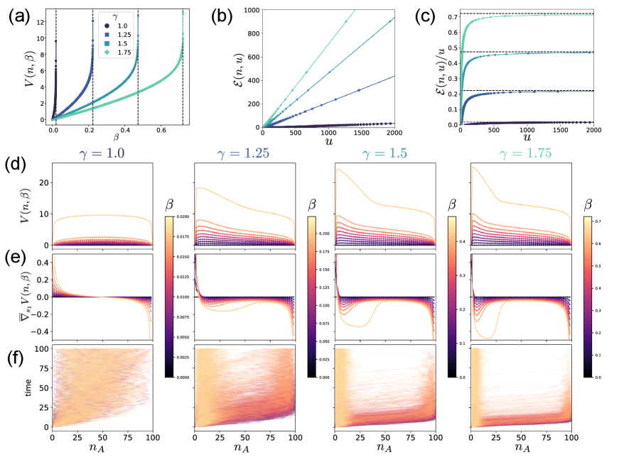
We numerically calculated the value function in two ways: by solving the linear algebraic Eq. (20) and by using the analytical formula in Eqs. (38)–(40). Two solutions exactly match, and the value function diverges as approaches the smallest eigenvalue (Fig. 3 (a)). The cost-exit time tradeoff curves in Fig. 3 (b) approach lines with slope in the long exit time regime. Thus, the cost rate per unit time is upper bounded by as shown in Fig. 3 (c). The result indicates that a finite amount of control cost per time is sufficient to prevent the ultimate extinction on average. As increases, the extinction tends to happen earlier, resulting in the increased control cost rate for preventing extinction.
As a function of , the value function for each and has a single peak, which we designate by (Fig. 3 (d)). The optimal control steers the system to stay around . As increases, the value gradient becomes steep around (Fig. 3 (e)) so that the controlled trajectories do not leave there even after a long time (Fig. 3 (f)).
When is close to , the width of the peak around decreases as increases, and there emerges a region with a shallow gradient . In this region, the optimal control become close to the uncontrolled rate . The emergence of the zero-gradient region indicates that the optimal control strategy switches between ON and OFF modes depending on the current state.
The OFF mode region appears if is high and is moderately large (see the Fig. S1 in Sec. E of the Supplementary Material [27]), implying that the OFF mode is attributed to the difficulty of controlling an exponentially growing population. If both and are large, the uncontrolled system has a stronger and less stochastic driving force towards as increases. Thus, the optimal control keeps the population away from by forcing it close to , which is the ON mode around the peak . Once a large fluctuation drives the population to leave the peak, the additional cost to bring it back to the peak does not pay for its success rate, leading to the OFF mode, i.e., do nothing, in the intermediate region. Finally, the control turns ON again near to hang on there. Such a spontaneous emergence of hierarchical control may not be identified within the LQG approximation, highlighting the importance of taking into account the unique properties of RN.
II.8 Controlling epidemic outbreak
Lastly, we apply our framework to epidemic problems. We use the stochastic SIR model (Fig. 1 (c)) in which the population is divided into three classes: susceptible (), infected (), and recovered (), i.e., . The uncontrolled process is described by the following infection and recovery reactions:
| (41) |
and we assume mass-action-type kinetics, i.e., and . The total population size is a conserved quantity of the system. This model has absorbing states and any stochastic solution eventually reaches one of these states as . When the ratio between reaction rate coefficients is high, the infection spreads rapidly in the population, and the state at the terminal time tends to have a small number of susceptible and a large number of recovered people. The number of recovered people at the end is equal to the total number of infections during the epidemic, which is known as the size of the epidemic [47].
The goal of control is then to minimize the size of the epidemic or, equivalently, to maximize the number of susceptible people at the end of the epidemic. Let us formulate it as the first exit problem where and , i.e.,
| (42) |
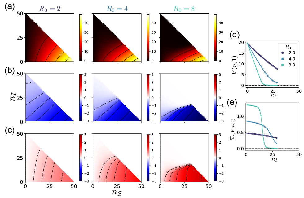
We numerically calculated the value function and the optimal reaction rate using Eqs. (20) and (13) for . The results are shown in Fig. 4. The value decreases as the number of susceptible people decreases and as the number of infected people increases (Fig. 4 (a)). The optimal control of infection and recovery rates plotted in Fig. 4 (b) and (c) indicates that strong control to reduce the infection rate and to boost the recovery rate is encouraged when the number of susceptibles is large and the number of infected is small. However, if many people are already infected, strong control is no longer encouraged. Instead, almost no control over the infection and recovery rates becomes optimal, as indicated by the white regions in Fig. 4 (b) and (c). This means that almost the entire population will eventually become infected in this situation, no matter how optimally the rates are controlled, and that further investment in the control cost is not worth the potential gains.
In particular, we can observe a sharp transition between strong control and no control when is high. Figures 4 (d) and (e) show the value function and its gradient on the line , which determines the optimal recovery rate . The value functions are approximately piecewise-linear functions , so the gradients and the optimal rates are approximately piecewise-constant. This transition leads to the mode switching of optimal control, which is similar to the case of the problem of maintaining diversity.
III Discussion
In this paper, we proposed a new framework to formulate optimal control problems of stochastic reaction networks. We showed that the Kullback–Leibler divergence has sound properties as the control cost of RN, taming the HJB equation via its linearization through Cole-Hopf transformation. It also yields a computationally efficient expression of the optimal solutions. We demonstrated the effectiveness of our framework for three classes of biological control problems with absorbing states.
There are several potential directions worth investigating. The first is risk-sensitive problems [48, 49], where not only the expectation of performance but also the variance and higher-order moments matter. For instance, as the concentration of intracellular molecules inevitably fluctuates, it is vital to suppress the fluctuation and variability when robust homeostasis is required [50]. As studied for diffusion processes [51], the current optimal control framework can be extended to incorporate risk sensitivity.
Second, more realistic reaction network models can have many types or large population sizes, such as complex ecological systems and stage-structured epidemic models [52, 53, 54, 55]. The optimal control problem for large models is accompanied by high-dimensional equations. Despite the linearity of the equation, solving it is numerically challenging. The development of fast and scalable numerical algorithms is essential for addressing large-scale problems. Sampling-based techniques [24, 56] would be efficient for these high-dimensional settings.
Finally, it would be desirable if we could modify the control cost function more flexibly depending on the setting of the actual control problem. For instance, if some components of the reaction rate coefficient are constrained to lie in a certain range, or if some reactions incur a much higher control cost than the others, the control cost function has to deviate from the Kullback–Leibler divergence, resulting in the loss of the efficient computation of the optimal solutions via Cole-Hopf transformation. This limitation is analogous to the inverse proportionality condition between the weight of control cost and the noise strength, being required to solve optimal control problems for diffusion processes efficiently [24, 26]. For stochastic reaction networks, the noise strength is related to the propensity function , which should be used as the weight of the control cost. An iterative method with local approximation as in [57, 58] might provide a way to overcome the limitation.
Acknowledgements.
We thank Simon Schnyder, Louis-Pierre Chaintron, and Kenji Kashima for their helpful discussions. This research is supported by JST CREST JPMJCR2011 and JPMJCR1927, and JSPS KAKENHI Grant Numbers 21J21415, 24KJ0090, 24H02148.References
- Bressloff [2014] P. C. Bressloff, Stochastic Processes in Cell Biology, Interdisciplinary Applied Mathematics, Vol. 41 (Springer International Publishing, 2014).
- Qian and Ge [2021] H. Qian and H. Ge, Stochastic Chemical Reaction Systems in Biology (Springer International Publishing, 2021).
- Lugagne et al. [2017] J.-B. Lugagne, S. Sosa Carrillo, M. Kirch, A. Köhler, G. Batt, and P. Hersen, Nature Communications 8, 1671 (2017).
- Gatenby et al. [2009] R. A. Gatenby, A. S. Silva, R. J. Gillies, and B. R. Frieden, Cancer Research 69, 4894 (2009).
- Sehl et al. [2011] M. Sehl, H. Zhou, J. S. Sinsheimer, and K. L. Lange, Mathematical Biosciences 234, 132 (2011).
- Raatz and Traulsen [2023] M. Raatz and A. Traulsen, Evolution 77, 1408 (2023).
- McKee and Chaudhry [2017] C. McKee and G. R. Chaudhry, Colloids and Surfaces B: Biointerfaces 159, 62 (2017).
- Ericsson and Franklin [2015] A. C. Ericsson and C. L. Franklin, ILAR Journal 56, 205 (2015), https://academic.oup.com/ilarjournal/article-pdf/56/2/205/9644116/ilv021.pdf .
- Woodland and Kohlmeier [2009] D. L. Woodland and J. E. Kohlmeier, Nature Reviews Immunology 9, 153 (2009).
- Sallusto et al. [2010] F. Sallusto, A. Lanzavecchia, K. Araki, and R. Ahmed, Immunity 33, 451 (2010), 21029957 .
- Rands et al. [2010] M. R. W. Rands, W. M. Adams, L. Bennun, S. H. M. Butchart, A. Clements, D. Coomes, A. Entwistle, I. Hodge, V. Kapos, J. P. W. Scharlemann, W. J. Sutherland, and B. Vira, Science 10.1126/science.1189138 (2010).
- Sarkar et al. [2006] S. Sarkar, R. L. Pressey, D. P. Faith, C. R. Margules, T. Fuller, D. M. Stoms, A. Moffett, K. A. Wilson, K. J. Williams, P. H. Williams, and S. Andelman, Annual Review of Environment and Resources 31, 123 (2006).
- Kuussaari et al. [2009] M. Kuussaari, R. Bommarco, R. K. Heikkinen, A. Helm, J. Krauss, R. Lindborg, E. Öckinger, M. Pärtel, J. Pino, F. Rodà, C. Stefanescu, T. Teder, M. Zobel, and I. Steffan-Dewenter, Trends in Ecology & Evolution 24, 564 (2009), 19665254 .
- Fischer et al. [2015] A. Fischer, I. Vázquez-García, and V. Mustonen, Proceedings of the National Academy of Sciences 112, 1007 (2015).
- Nourmohammad and Eksin [2021] A. Nourmohammad and C. Eksin, Physical Review X 11, 011044 (2021).
- Piret and Boivin [2021] J. Piret and G. Boivin, Frontiers in Microbiology 11, 10.3389/fmicb.2020.631736 (2021).
- Aurell et al. [2022] A. Aurell, R. Carmona, G. Dayanikli, and M. Laurière, SIAM Journal on Control and Optimization 60, S294 (2022).
- Schnyder et al. [2023] S. K. Schnyder, J. J. Molina, R. Yamamoto, and M. S. Turner, PLOS Computational Biology 19, e1011533 (2023).
- Gardiner [2009] C. Gardiner, Stochastic Methods, 4th ed. (Springer Berlin, Heidelberg, 2009).
- Anderson and Kurtz [2011] D. F. Anderson and T. G. Kurtz, in Design and Analysis of Biomolecular Circuits: Engineering Approaches to Systems and Synthetic Biology (Springer, 2011) pp. 3–42.
- Fleming and Mitter [1982] W. H. Fleming and S. K. Mitter, Stochastics 8, 63 (1982).
- Mitter and Newton [2003] S. K. Mitter and N. J. Newton, SIAM Journal on Control and Optimization 42, 1813 (2003).
- Todorov [2008] E. Todorov, in 2008 47th IEEE Conference on Decision and Control (IEEE, 2008) pp. 4286–4292.
- Kappen [2005] H. J. Kappen, Journal of Statistical Mechanics: Theory and Experiment 2005, P11011 (2005).
- Fleming and Soner [2006] W. H. Fleming and H. M. Soner, Controlled Markov Processes and Viscosity Solutions, Vol. 25 (Springer-Verlag, 2006).
- Todorov [2009] E. Todorov, Proceedings of the National Academy of Sciences 106, 11478 (2009).
- Note [1] See Supplemental Material at for the derivation of equations and detailed numerical results, which includes Refs. [59, 60, 61, 62, 63, 64].
- Lorch et al. [2018] L. Lorch, A. De, S. Bhatt, W. Trouleau, U. Upadhyay, and M. Gomez-Rodriguez, Stochastic Optimal Control of Epidemic Processes in Networks (2018), 1810.13043 .
- Theodorou and Todorov [2012a] E. A. Theodorou and E. Todorov, in 2012 American Control Conference (ACC) (IEEE, 2012) pp. 1633–1639.
- Okumura et al. [2017] Y. Okumura, K. Kashima, and Y. Ohta, Asian Journal of Control 19, 781 (2017).
- Horiguchi and Kobayashi [2023] S. A. Horiguchi and T. J. Kobayashi, Physical Review Research 5, L022052 (2023).
- Kipnis and Landim [1999] C. Kipnis and C. Landim, Scaling Limits of Interacting Particle Systems, Vol. 320 (Springer Berlin Heidelberg, 1999).
- Theodorou and Todorov [2012b] E. A. Theodorou and E. Todorov, in 2012 IEEE 51st IEEE Conference on Decision and Control (CDC) (IEEE, 2012) pp. 1466–1473.
- Gao et al. [2023] Y. Gao, J.-G. Liu, and O. Tse, Optimal control formulation of transition path problems for Markov Jump Processes (2023), 2311.07795 .
- Guéant [2020] O. Guéant, Optimal control on finite graphs: Asymptotic optimal controls and ergodic constant in the case of entropic costs (2020).
- Jaimungal et al. [2024] S. Jaimungal, S. M. Pesenti, and L. Sánchez-Betancourt, SIAM Journal on Control and Optimization 62, 982 (2024).
- Xie [2020] P. Xie, ACS Omega 5, 5721 (2020).
- Feller [1966] W. Feller, SIAM Journal on Applied Mathematics 14, 864 (1966), 2946141 .
- Karlin and McGregor [1959] S. Karlin and J. McGregor, Pacific Journal of Mathematics 9, 1141 (1959).
- Fisher [1984] M. E. Fisher, Journal of Statistical Physics 34, 667 (1984).
- Katori and Tanemura [2007] M. Katori and H. Tanemura, Journal of Statistical Physics 129, 1233 (2007).
- Moran [1958] P. A. P. Moran, Annals of Human Genetics 23, 1 (1958).
- Karlin and McGregor [1967] S. Karlin and J. McGregor, Proc. 5th Berkeley Symp. Math. Stat. Prob. 4, 415 (1967).
- Houchmandzadeh and Vallade [2010] B. Houchmandzadeh and M. Vallade, Physical Review E 82, 051913 (2010).
- Ashcroft et al. [2015] P. Ashcroft, A. Traulsen, and T. Galla, Physical Review E 92, 042154 (2015).
- Hershkowitz et al. [1987] D. Hershkowitz, V. Mehrmann, and H. Schneider, Linear Algebra and its Applications 88–89, 373 (1987).
- Bailey [1953] N. T. J. Bailey, Biometrika 40, 177 (1953), 2333107 .
- Jacobson [1973] D. Jacobson, IEEE Transactions on Automatic Control 18, 124 (1973).
- Whittle [1990] P. Whittle, Risk Sensitive Optimal Control, Wiley-Interscience Series in Systems and Optimization (Wiley, 1990).
- Raser and O’Shea [2005] J. M. Raser and E. K. O’Shea, Science 309, 2010 (2005).
- van den Broek et al. [2010] B. van den Broek, W. Wiegerinck, and H. Kappen, in Conference on Uncertainty in Artificial Intelligence (2010).
- Xiao et al. [2020] Y. Xiao, M. T. Angulo, S. Lao, S. T. Weiss, and Y.-Y. Liu, Nature Communications 11, 3329 (2020).
- Skwara et al. [2023] A. Skwara, K. Gowda, M. Yousef, J. Diaz-Colunga, A. S. Raman, A. Sanchez, M. Tikhonov, and S. Kuehn, Nature Ecology & Evolution 10.1038/s41559-023-02197-4 (2023).
- Brauer and Castillo-Chavez [2012] F. Brauer and C. Castillo-Chavez, Mathematical Models in Population Biology and Epidemiology, Texts in Applied Mathematics, Vol. 40 (Springer New York, 2012).
- D’Souza et al. [2023] R. M. D’Souza, M. Di Bernardo, and Y.-Y. Liu, Nature Reviews Physics 5, 250 (2023).
- Theodorou et al. [2010] E. Theodorou, J. Buchli, and S. Schaal, in 2010 IEEE International Conference on Robotics and Automation (IEEE, 2010) pp. 2397–2403.
- Todorov and Weiwei Li [2005] E. Todorov and Weiwei Li, in Proceedings of the 2005, American Control Conference, 2005. (IEEE, 2005) pp. 300–306.
- Satoh et al. [2017] S. Satoh, H. J. Kappen, and M. Saeki, IEEE Transactions on Automatic Control 62, 262 (2017).
- Boel and Varaiya [1977] R. Boel and P. Varaiya, SIAM Journal on Control and Optimization 15, 92 (1977).
- Boyd and Vandenberghe [2004] S. P. Boyd and L. Vandenberghe, Convex Optimization (Cambridge University Press, 2004).
- Opper and Sanguinetti [2007] M. Opper and G. Sanguinetti, in Advances in Neural Information Processing Systems, Vol. 20 (Curran Associates, Inc., 2007).
- Nakamura and Kobayashi [2022] K. Nakamura and T. J. Kobayashi, Physical Review Research 4, 013120 (2022).
- Xianping Guo and Hernandez-Lerma [2003] Xianping Guo and O. Hernandez-Lerma, IEEE Transactions on Automatic Control 48, 236 (2003).
- Feller [1991] W. Feller, An Introduction to Probability Theory and Its Applications, 3rd ed., Vol. Volume 1 (Wiley, 1991).