Optimal design of large-scale nonlinear Bayesian inverse problems under model uncertainty
Abstract
We consider optimal experimental design (OED) for Bayesian nonlinear inverse problems governed by partial differential equations (PDEs) under model uncertainty. Specifically, we consider inverse problems in which, in addition to the inversion parameters, the governing PDEs include secondary uncertain parameters. We focus on problems with infinite-dimensional inversion and secondary parameters and present a scalable computational framework for optimal design of such problems. The proposed approach enables Bayesian inversion and OED under uncertainty within a unified framework. We build on the Bayesian approximation error (BAE) approach, to incorporate modeling uncertainties in the Bayesian inverse problem, and methods for A-optimal design of infinite-dimensional Bayesian nonlinear inverse problems. Specifically, a Gaussian approximation to the posterior at the maximum a posteriori probability point is used to define an uncertainty aware OED objective that is tractable to evaluate and optimize. In particular, the OED objective can be computed at a cost, in the number of PDE solves, that does not grow with the dimension of the discretized inversion and secondary parameters. The OED problem is formulated as a binary bilevel PDE constrained optimization problem and a greedy algorithm, which provides a pragmatic approach, is used to find optimal designs. We demonstrate the effectiveness of the proposed approach for a model inverse problem governed by an elliptic PDE on a three-dimensional domain. Our computational results also highlight the pitfalls of ignoring modeling uncertainties in the OED and/or inference stages.
MnLargeSymbols’164 MnLargeSymbols’171
Keywords: Optimal experimental design, sensor placement, Bayesian inverse problems, model uncertainty, Bayesian approximation error.
1 Introduction
Models governed by partial differential equations (PDEs) are common in science and engineering applications. Such PDE models often contain parameters that need to be estimated using observed data and the model. This requires solving an inverse problem. The quality of the estimated parameters is influenced significantly by the quantity and quality of the measurement data. Therefore, optimizing the data acquisition process is crucial. This requires solving an optimal experimental design (OED) problem [7, 13, 43]. In the present work, we focus on inverse problems in which measurement data are collected at a set of sensors. In this case, OED amounts to finding an optimal sensor placement. In this context, OED is especially important when only a few sensors can be deployed.
While some parameters in the governing PDEs can be estimated by solving an inverse problem, often there are additional uncertain model parameters that are not being estimated. These parameters might be too costly or impossible to estimate. We call the uncertain parameters that are being estimated in an inverse problem the inversion parameters and refer to the additional uncertain parameters as the secondary parameters. Such secondary parameters have also been referred to as auxiliary parameters, latent parameters, or nuisance parameters in the literature. When solving inverse problems with secondary parameters with significant uncertainty levels, both the parameter estimation and data acquisition processes need to be aware of such uncertainties. In this article, we present a computational framework for optimal design of nonlinear Bayesian inverse problems governed by PDEs under model uncertainty.
Uncertainties in mathematical models can be divided into two classes: reducible and irreducible [39]. The reducible uncertainties are epistemic uncertainties that can be reduced via statistical parameter estimation. On the other hand, irreducible uncertainties are either aleatoric uncertainties inherent to the model that are impossible to reduce or are epistemic uncertainties that are too costly or impractical to reduce. Also, in some applications we might have access to a probabilistic description of secondary model parameters from previous studies and further reduction of the uncertainty in such parameters may not be worth the additional computational cost. We consider such uncertainties as irreducible as well. In the present work, we focus on the case of irreducible uncertainties.
We consider models of the form
| (1) |
where is a vector of measured data, is a PDE-based model, and are uncertain parameters, and is a random vector that models measurement noise. Herein, is the inversion parameter which we seek to infer, and is a secondary uncertain model parameter. We assume the uncertainty in to be irreducible. The parameters and are assumed to be independent random variables that take values in infinite-dimensional real separable Hilbert spaces and , respectively. Moreover, is assumed to be nonlinear in both and . The methods presented in this article enable computing optimal experimental designs in such a way that the uncertainty in the secondary parameters is accounted for.
Related work
In the recent years, there have been numerous research efforts directed at OED in inverse problems governed by PDEs. See the review [1], for a survey of the recent literature in this area. There has also been an increased interest in parameter inversion and design of experiments in systems governed by uncertain forward models; see e.g., [27, 6, 24, 33, 14, 38] for a small sample of the literature addressing inverse problems under uncertainty. Methods for OED in such inverse problems have been studied in [28, 5, 18, 11]. The works [28, 5] concern optimal design of infinite-dimensional Bayesian linear inverse problems governed by PDEs. Specifically, [28] considers design of linear inverse problems governed by PDEs with irreducible sources of model uncertainty. On the other hand, [5] targets OED for linear inverse problems with reducible sources of uncertainty. The efforts [18, 11] focus on inverse problems with finite- and low-dimensional inversion and secondary parameters. These articles devise sampling approaches for estimating the expected information gain in such problems. The setting considered in [18] is that of inverse problems with reducible uncertainties. The approach in [11] employs a small noise approximation that applies to problems with nuisance parameters that have small uncertainty levels.
Our approach
We focus on Bayesian nonlinear inverse problems governed by PDEs with infinite-dimensional inversion and secondary parameters. Traditionally, when solving such inverse problems all the secondary model parameters are fixed at their nominal values and the focus is on the estimation of the inversion parameters. Considering 1, this amounts to using the approximate model , where is some nominal value. In Section 2, we consider simpler instances of 1 and illustrate the role of model uncertainty in Bayesian inverse problems and the importance of accounting for such uncertainties in parameter inversion and OED. The discussion in Section 2 motivates our approach for incorporating secondary uncertainties in nonlinear Bayesian inverse problems and the corresponding OED problems. This is done using the Bayesian approximation error (BAE) approach [26, 24]; see Section 3.
Subsequently, we build on methods for optimal design of infinite-dimensional nonlinear inverse problems [4, 44, 1] to derive an uncertainty aware OED objective. Specifically, we follow an A-optimal design strategy where the goal is to obtain designs that minimize average posterior variance. To cope with the non-Gaussianity of the posterior, we rely on a Gaussian approximation to the posterior. This enables deriving approximate measures of posterior uncertainty that are tractable to optimize for infinite-dimensional inverse problems; see Section 4. We then present two approaches for formulating and computing the OED objective; see Section 5. The first approach uses Monte Carlo trace estimators and the second one formulates the OED problem as an eigenvalue optimization problem. In each case, the OED problem is formulated as a bilevel binary PDE-constrained optimization problem. In both approaches, the cost of computing the OED objective, in terms of the number of PDE solves, is independent of the dimensions of discretized inversion and secondary parameters. This makes these approaches suitable for large-scale applications. In the present work, we rely on a greedy approach to solve the resulting optimization problems. As discussed in Section 5, a greedy algorithm is especially suited for the formulation of the OED problem in Section 5.2.2, as a binary PDE-constrained eigenvalue optimization problem.
We elaborate the proposed approach in the context of a model inverse problem governed by an elliptic PDE in a three-dimensional domain; see Section 6. This inverse problem, which is motivated by heat transfer applications, concerns estimation of a coefficient field on the bottom boundary of the domain, using sensor measurements of the temperature on the top boundary. The secondary uncertain parameter in this inverse problem is the log-conductivity field, which is modeled as a random field on the three-dimensional physical domain. Our computational results in Section 7 demonstrate the effectiveness of the proposed strategy in computing optimal sensor placements under model uncertainty. We also systematically study the drawbacks of ignoring the uncertainty in the Bayesian inversion and experimental design stages. These studies illustrate the fact that ignoring uncertainty in OED or inference stages can lead to inferior designs and highly inaccurate results in parameter estimation.
Contributions
The contributions of this article are as follows: (1) We present an uncertainty aware formulation of the OED problem, uncertainty aware OED objectives along with scalable methods for computing them, and an extensible optimization framework for computing optimal designs. These make OED for nonlinear Bayesian inverse problems governed by PDEs with infinite-dimensional inversion and secondary parameters feasible. Additionally, the proposed approach enables Bayesian inversion and OED under uncertainty within a unified framework. (2) We elaborate the proposed approach for an inverse problem governed by an elliptic PDE, on a three-dimensional domain, with infinite-dimensional inversion and secondary parameters. This is used to elucidate the implementation of our proposed approach for design of inverse problems governed by PDEs under uncertainty. (3) We present comprehensive computational studies that illustrate the effectiveness of the proposed approach and also the importance of accounting for modeling uncertainties in both parameter inversion and experimental design stages. (4) By considering simpler instances of 1, in Section 2, we present a systematic study of the role of model uncertainty in Bayesian inverse problems and the importance of accounting for such uncertainties in parameter inversion and OED. That study also reveals a connection between the BAE-based approach taken in the present work and the method for OED in linear inverse problems under uncertainty in [5].
The developments in this article point naturally to a number of extensions of the presented methods. We discuss such issues in Section 8, where we present our concluding remarks, and discuss potential limitations of the presented approach and opportunities for future extensions.
2 Motivation and overview
In this section, we motivate our approach for OED under uncertainty and set the stage for the developments in the rest of the article. After a brief coverage of requisite notation and preliminaries in Section 2.1, we begin our discussion in Section 2.2 by considering a simple form of 1 where is linear in and . This facilitates an intuitive study of the role of model uncertainty in Bayesian inverse problems and OED. We then consider nonlinear models of varying complexity in Section 2.3 to motivate our approach for design of inverse problems governed by nonlinear models of the form 1.
2.1 Preliminaries
In this article, we consider inversion and secondary parameters that take values in infinite-dimensional Hilbert spaces. For a Hilbert space , we denote the corresponding inner product by and the associated induced norm by ; i.e., . For Hilbert spaces and , denotes the space of bounded linear transformations from to . The space of bounded linear operators on a Hilbert space is denoted by , and the subspace of bounded selfadjoint operators is denoted by . We let denote the set of bounded positive selfadjoint operators. The subspace of trace-class operators in is denoted by , and the subspace of selfadjoint trace-class operators is denoted by . Also, the sets of positive and strictly positive selfadjoint trace-class operators are denoted by and , respectively.
Throughout the article, denotes a Gaussian measure with mean and covariance operator . For a Gaussian measure on an infinite-dimensional Hilbert space , the covariance operator is required to be in . Herein, we consider non-degenerate Gaussian measures; i.e., we assume that . For further details on Gaussian measures, we refer to [15, 40]. Also, when considering measures on Hilbert spaces, we equip these spaces with their associated Borel sigma algebra. Throughout the article, for notational convenience, we suppress this choice of the sigma-algebra in our notations.
The adjoint of a linear transformation , where and are (real) Hilbert spaces, is denoted by . Recall that and
We also recall the following basic result regarding affine transformations of Gaussian random variables. Let be an -valued Gaussian random variable with law , , and . Then, the random variable is an -valued Gaussian random variable with law ; see [15] for details.
2.2 Linear models
Consider the model
| (2) |
where denotes measurement data, is the inversion parameter, is the secondary uncertain parameter, and is the measurement noise vector. (The spaces and are as described in the introduction.) This type of model, which was considered in [5], may correspond to inverse problems governed by linear PDEs with uncertainties in source terms or boundary conditions. We assume and . Moreover, we assume that and that is independent of and . We consider a Gaussian prior law for , and for the purpose of this illustrative example, let the secondary model uncertainty be distributed according to a Gaussian . Also, we assume , with denoting the noise level.
Incorporating model uncertainty in the inverse problem
For a fixed realization of , estimating from 2 is a standard problem. This also follows the common practice of fixing additional model parameters at some nominal values before solving the inverse problem. However, it is possible to account for the model uncertainty in this process. To see this, suppose we fix at and consider the approximate model . Note that
In this case, the approximation error has a Gaussian law, . Hence, we may rewrite 2 in terms of the approximate model as follows:
| (3) |
where denotes the total error. In the present setting, . Note that we have incorporated the uncertainty due to in the error covariance matrix.111 If the approximate model was defined by fixing at a point different from , then the error term would have nonzero mean. The present procedure for incorporating the secondary model uncertainty into the inverse problem is a special case of the Bayesian approximation error (BAE) approach (see section 3).
Since we have Gaussian prior and noise models and in 3 is affine, the posterior is also Gaussian with analytic formulas for its mean and covariance operator; see e.g., [40]. In particular, the posterior covariance operator is given by
| (4) |
Considering, for example, the A-optimality criterion , 4 illustrates the manner in which the uncertainty due to use of an approximate model impacts the posterior uncertainty.
Interplay between measurement error and approximation error
Note that . This operator admits a spectral decomposition , where is an orthogonal matrix of eigenvectors and is a diagonal matrix with the eigenvalues on it diagonal. Thus, the total error covariance matrix can be written as . Therefore, the modes for which may be ignored. To observe the impact of model uncertainty on individual observations, we note that
where ’s are the standard basis vectors in . Thus, we see that only large eigenvalues contribute significantly to the total error in the th measurement.
We can also consider the interplay between the spectral representation of the error covariance and the posterior covariance operator. Specifically, with . Thus, letting , , we can write
Note that in the directions corresponding to very large eigenvalues the measurements will have a negligible impact on posterior uncertainty.
The above discussion indicates that model uncertainty cannot be ignored in the inverse problem, especially when the model uncertainty overwhelms measurement noise. The latter is also important in design of experiments. Specifically, some of the measurements might be completely useless due to large amount of model uncertainty associated to the corresponding measurements. This information needs to be accounted for in the OED problem to ensure only measurements that are helpful in reducing posterior uncertainty are selected.
Connection to post-marginalization
In general, the BAE approach involves pre-marginalization over the secondary model uncertainties. This can be related to the idea of post-marginalization in the case of linear Gaussian inverse problems. Namely, if we consider as a reducible uncertainty that is being estimated along with and as the corresponding prior law, then 4 is the covariance operator of the marginal posterior law of . To see this, we first note that
| (5) |
This relation can be derived by following a similar calculation as the one in [40, p. 536].222 Note that 5 can be viewed as a special form of the Sherman–Morrison–Woodbury formula involving Hilbert space operators. Then, we substitute 5 in 4 to obtain
This is the same as the marginal posterior covariance operator of as noted in [5, Equation 2.4]. Thus, for a linear Gaussian inverse problem with reducible secondary uncertainty, the posterior covariance operator obtained using the BAE approach equals the marginal posterior covariance operator of obtained following joint estimation of and .
2.3 Nonlinear models
The linear model 2 can be generalized in the following ways:
| (6) | |||
| (7) | |||
| (8) | |||
| nonadditive model, nonlinear in both and . | (9) |
While the cases 6–8 might be of independent interest, our focus in this article is on the general case 9. However, items 6–8 do serve to illustrate some of the key challenges.
In the case of 6, one can repeat the steps leading to 3, except will not be Gaussian anymore and therefore the distribution of will not be known analytically. In that case, one may obtain a Gaussian approximation to either by fitting a Gaussian to or by using a linear approximation of . Then, one may obtain a Gaussian posterior, where one also relies on the linearity of . On the other hand, in the case of 7, the total error will be Gaussian as before, but due to nonlinearity of the posterior will not be Gaussian. The latter leads to one of the fundamental challenges in OED of nonlinear inverse problem—defining a suitable OED objective whose optimization is tractable. The more complicated cases of 8—9 inherit the challenges corresponding to the previous cases.
In the rest of this article, we build on the BAE approach to incorporate the uncertainty in in inverse problems governed by nonlinear models of the type 9. The uncertainty in will be assumed irreducible, and in general, will not be assumed to follow a Gaussian law. All that we require is the ability to generate samples of . Following the BAE approach, we approximate the approximation error with a Gaussian. This enables incorporating the model uncertainty in the data likelihood; see Section 3. To cope with non-Gaussianity of the posterior, we rely on a Gaussian approximation to the posterior, to derive an uncertainty aware OED objective that is tractable to evaluate and optimize for infinite-dimensional inverse problems; see Section 4 for the definition of the OED objective and Section 5 for computational methods.
3 Infinite-dimensional Bayesian inverse problems under uncertainty
We consider the inverse problem of inferring a parameter from a model of the form 1, where is a parameter-to-observable map that in general is nonlinear in both arguments. We focus on problems where is defined as a composition of an observation operator and a PDE solution operator. The model is assumed to be Fréchet differentiable in , at , where is a nominal value. As before, we employ a Gaussian noise model, , a Gaussian prior law for , and assume is independent of and . The prior induces the Cameron–Martin space , which is endowed with the inner product [15, 17]
where is the inner product on the parameter space .
To account for model uncertainty (due to ) in the inverse problem, we rely on the BAE approach [26, 24], which we explain next. We fix the secondary parameter to and consider the approximate (also known as inaccurate, reduced order, or surrogate) model
| (10) |
As mentioned before, this is typically what is done in practice where the secondary model parameters are fixed at some (possibly well-justified) nominal values. In the BAE approach, we quantify and incorporate errors due to the use of this approximate model in the Bayesian inverse problem analogously to what was done in Section 2.2. Namely, we consider
| (11) |
where is the total error. In the BAE framework, the approximation error , is approximated as a conditionally Gaussian random variable. That is, the distribution of is assumed to be Gaussian. In the present work, we employ the so-called enhanced error model [27, 24, 10], that ignores the correlation between and and approximates the law of as a Gaussian with
| (12) | ||||
In general, the approximation errors can be (highly) correlated with the parameters [34, 24]. However, ignoring the correlation between and (i.e., employing the enhanced error model) is typically viewed as a conservative (safe) approximation as it is analogous to approximating the conditional distribution of with the marginal distribution of , which cannot reduce variance [25, Section 3.4]. On the other hand, employing the enhanced error model can significantly reduce the costs associated with computing the mean and covariance operator of [24] which are in practice computed via sampling; see Section 5.
With these approximations, and by our assumption on the measurement noise (which is independent of the parameters), the total error is modeled by a Gaussian , where . Using this approximate noise model along with the approximate model we arrive at the following data likelihood:
| (13) |
With the prior measure in place, and using this BAE-based data likelihood, we can state the Bayes formula [40],
To make computations involved in design of large-scale inverse problems tractable, we rely on a local Gaussian approximation to the posterior. Namely, we use , where is the maximum a posteriori probability (MAP) point and is an approximate posterior covariance operator, described below. The MAP point is given by
| (14) |
For the approximate posterior covariance operator , we use
| (15) |
where is the Fréchet derivative of evaluated at .
Note that the true posterior is equivalent to the prior measure. It is also possible to show that the Gaussian approximation is equivalent to , as well. This fact, which is made precise below, is important in justifying the use of this Gaussian approximation for defining an approximate measure of posterior uncertainty. Namely, to define a notion of uncertainty reduction, it is important that our surrogate for the posterior measure is absolutely continuous with respect to our reference measure, which is given by the prior. The equivalence of to may be inferred from the more general developments in [35]. However, we present an accessible argument that applies to the specific problem setup under study in the present work. We first present the following result.
Proposition 3.1.
Consider the linearized forward model
| (16) |
where we have suppressed the dependence of to for notational convenience. Define the data model
| (17) |
where . Consider the Bayesian inverse problem of estimating using 17 and the prior . The corresponding posterior measure is given by .
Proof.
Using the theory of Bayesian linear inverse problems in a Hilbert space [40], the solution of the linear inverse problem under study yields a Gaussian posterior . The covariance operator is as in 15 and is found by minimizing
| (18) |
over the Cameron–Martin space . To complete the proof, we show . Note that is a strictly convex quadratic functional with a unique global minimizer. We consider the Euler–Lagrange equation for the present optimization problem. Note that the Fréchet derivative of is given by . It is straightforward to see
for every . Thus, recalling , we note that for every ,
The last equality follows from the fact that is a minimizer of in 14. Hence, is the unqiue global minimizer of . Therefore, . ∎
Proposition 3.1 shows that is the posterior measure corresponding to the linearized Bayesian inverse problem considered in the result. Therefore, by construction, is equivalent to .
4 A-optimal experimental design under uncertainty
We consider inverse problems in which measurement data are collected at a set of sensors. In this case, the OED problem seeks to find an optimal placement of sensors. Specifically, we formulate the OED problem as that of selecting an optimal subset from a set of candidate sensor locations, which is a common approach; see e.g., [43, 20, 3]. To make matters concrete, we begin by fixing a set of points that indicate the candidate sensor locations. We then assign a binary weight to each candidate location ; a weight of one indicates that a sensor will be placed at the corresponding candidate location. The binary vector thus fully specifies an experimental design in the present setting. Note that specification of a set of candidate sensor locations will in general depend on the specific application at hand. For example, placing sensors in certain parts of the domain might be impractical or impossible. Also, in problems with Dirichlet boundary conditions, placing sensors on or very close to such boundaries will be a waste of resources.
4.1 Design of the Bayesian inverse problem
The design enters the formulation of the Bayesian inverse problem through the data likelihood. This requires additional care in the present work because the total error covariance matrix is non-diagonal. We follow the setup in [31] to incorporate in the Bayesian inverse problem formulation. For a binary design vector , we define the matrix as submatrix of with rows corresponding to the zero weights removed. Thus, given a generic measurement vector , returns the measurements corresponding to active sensors. For , we use the notation .
Next, we describe how a design vector enters the Bayesian inverse problem, within the BAE framework. For a given , we consider the model . Using this model leads to the following, -dependent, data likelihood
| (19) |
with
| (20) |
Consequently, we obtain the following -dependent Gaussian approximation to the posterior, , where is obtained by minimizing
| (21) |
and
| (22) |
4.2 The design criterion
In the present work, we follow an A-optimal design strategy, where the goal is to find designs that minimize the average posterior variance. Generally, computing the average posterior variance for a Bayesian nonlinear inverse problem is computationally challenging. We follow the developments in [4] to define a Bayesian A-optimality criterion in the case of nonlinear inverse problems.
Given a data vector , an approximate measure of posterior uncertainty is provided by . However, when solving the OED problem data is not available. Indeed, it is the goal of the OED problem to specify how data should be collected. To overcome this, we follow the general approach in Bayesian OED of nonlinear inverse problems, where we consider , with denoting expectation with respect to the set of all likely data. We compute this expectation by using the information available in the Bayesian inverse problem and the information regarding the distribution of the model uncertainty. Namely, following the approach in [4], we use the design criterion
| (23) |
where is the probability density function (pdf) of the noise distribution . In practice, will be computed via sample averaging. Specifically, we use
| (24) |
where the training data samples are given by , with a sample set from the product space . In large-scale applications, typically a small can be afforded. However, in this context, typically a modest enables computing good quality optimal designs. This is also demonstrated in the computational results in the present work.
Note that, for each ,
where is a complete orthonormal set in . Inserting this in 24 and using the definition of , we have
| (25a) | |||
| where, for and , | |||
| (25b) | |||
| (25c) | |||
Computing the OED objective as defined above is not practical. However, 25 provides insight into the key challenges in computing the OED objective. In the first place, 25b is a challenging PDE-constrained optimization problem whose solution is the MAP point . Moreover, upon discretization, 25c will be a high-dimensional linear system with the discretization of the operator as its coefficient matrix. Such systems can be tackled with Krylov iterative methods that require the application of the coefficient matrix on vectors. In Section 5, we present two approaches for efficiently computing the OED objective: one approach uses randomized trace estimation and the other utilizes low-rank approximation of . These approaches rely on scalable optimization methods for 25b as well as adjoint based gradient and Hessian apply computation.
4.3 The optimization problem for finding an A-optimal design
We state the OED problem of selecting the best sensors, with , as follows:
| (26) | ||||
This is a challenging binary optimization problem. One possibility is to pursue a relaxation strategy [31, 3, 4] to enable gradient-based optimization with design weights . A practical alternative is to follow a greedy approach to find an approximate solution to 26. Namely, we place sensors one at a time. In each step of a greedy algorithm, we select the sensor that provides the largest decrease in the value of the OED objective . While the solutions obtained using a greedy algorithm are suboptimal in general, greedy approaches have shown good performance in many sensor placement problems; see, e.g., [29, 37, 23, 5]. In the present work, we follow a greedy approach for finding approximate solutions for 26. The effectiveness of this approach is demonstrated in our computational results in Section 7.
5 Computational methods
We begin this section with a brief discussion on computing the BAE error statistics in Section 5.1. We then detail our proposed methods for computing the OED objective in Section 5.2. The greedy approach for computing optimal designs is outlined in Section 5.3. Then, we discuss the computational cost of OED objective evaluation, using our proposed methods, as well as the greedy procedure in Section 5.4.
5.1 Estimating approximation error statistics
As discussed in Section 3, the mean and covariance of the approximation error in 12 will be approximated via Monte Carlo sampling. Specifically, we begin by drawing samples in and compute
| (27) |
Subsequently, we use and . The computational cost of this process is model evaluations. Note, however, that these model evaluations are done a priori, in parallel, and can be used for both the OED problem and solving the inverse problem. Typically, only a modest sample size is sufficient for approximating the mean and covariance of the model error [33, 10]. Specifically, as noted in Section 2, only dominant modes of the error covariance matrix need to be resolved. Note also that (a subset of) the model evaluations in 27 may be reused in generation of training data needed for computation of the OED objective.
5.2 Computation of the OED objective
In this section, we present scalable computational methods for computing the OED objective. Specifically, we present two methods: (i) a method based on the use of randomized trace estimators (Section 5.2.1) and (ii) a method based on low-rank spectral decompositions (Section 5.2.2). As discussed further below, the latter is particularly suited to our overall approach in the present work. Therefore, we primarily focus on the method based on low-rank spectral decompositions, which we also fully elaborate in the context of a model inverse problem (see Section 6 and Section 7). However, the first method does have its own merits and is included to provide an alternative approach. The relative benefits and computational complexity of these methods are discussed in Section 5.4.
Before we proceed further, we define some notations that simplify the discussions that follow. For , we define
| (28) |
Note that the operator is the so-called Gauss–Newton Hessian of the data mistfit term in the definition of in 21, evaluated at .
5.2.1 Monte Carlo trace estimator approach
We begin by deriving a randomized (Monte Carlo) trace estimator for the posterior covariance operator 22. This is facilitated by the following technical result.
Proposition 5.1.
Let and , and consider the Gaussian measure on . Then, .
Proof.
By the assumptions on and , we have that both and are trace-class. Also, by the formula for the expectation of a quadratic form in the infinite-dimensional Hilbert space setting [2, Lemma 1], we have that . To finish the proof, we let be the (orthonormal) basis of the eigenvectors of with corresponding (real, positive) eigenvalues , and note ∎
Next, note that we can write as
| (29) |
Using this and letting and in Proposition 5.1, we have . Approximating the integral on the right hand side via sampling, we obtain
where are draws from the measure . This randomized (Monte Carlo) trace estimator allows approximating the OED objective 24, as follows.
| (30a) | |||
| where, for and , | |||
| (30b) | |||
| (30c) | |||
The major computational challenge in computing is solving the MAP estimation problems in 30b. These inner optimization problems can be solved efficiently using an inexact Newton-Conjugate Gradient (Newton-CG) method. The required first and second order derivatives can be obtained efficiently using adjoint-based gradient and Hessian apply computation. The Hessian solves in 30c are also done using (preconditioned) CG. This only requires the action of on vectors, which can be done using the adjoint method. A detailed study of the computational cost of computing is provided in Section 5.4.
5.2.2 Low-rank approximation approach
Due to the use of finite-dimensional observations, in 28 has a finite-dimensional range. Also, often exhibits rapid spectral decay and, in cases where the dimension of measurements is high, the numerical rank of this operator is typically much smaller than its exact rank. Note that the exact rank is bounded by the measurement dimension. Such low-rank structures are due to possible smoothing properties of the forward operator and that of ; see, e.g., [12]. The following technical result facilitates exploiting such low-rank structures to compute the OED objective.
Proposition 5.2.
Let and be in . Letting be the orthonormal basis of eigenvectors of with corresponding (real non-negative) eigenvalues , we have
| (31) |
Proof.
The result follows by noting that
∎
The relation 31 facilitates approximating . Namely, we can truncate the infinite summation in the right-hand side to the first terms, corresponding to the dominant eigenvalues of . We can also quantify the approximation error due to this truncation as follows.
Proposition 5.3.
Let and be as in proposition 5.2 and let be the largest eigenvalues of . Define . Then,
| (32) |
Proof.
We have
Next, we consider and let be its dominant eigenpairs. (The dependence of eigenvalues and eigenvectors on is suppressed, for notational convenience.) Using Proposition 5.2 with and , we obtain the approximation
| (33) | ||||
Observe that only the second term in the right-hand side depends on . This term, which provides a measure of uncertainty reduction, can be used to define the OED objective. Specifically, using 24 along with (33), leads to following form of the OED objective:
| (34a) | ||||
| where, for , | ||||
| (34b) | ||||
| (34c) | ||||
| (34d) | ||||
Note that the numerical rank of will, in general, depend on . In 34, we have used a common target rank for simplicity. In the present setting, this target rank is bounded by the number of active sensors for a given . Note also that Proposition 5.3 shows how to quantify the error due to the use of truncated spectral decompositions. Namely, in view of 32, the error due to the truncation is bounded by .
As in the case of the approach outlined in Section 5.2.1, the dominant computational challenge in computing is the solution of the MAP estimation problems 34b. This will be tackled using the same techniques. The eigenvalue problem 34c can be tackled via Lanczos or randomized approaches. The target rank , can be selected as the number of active sensors. This is suitable in cases where we have a small number of active sensors. See Section 5.4 for further details regarding the computational cost of evaluating .
We point out that if the dominant eigenvalues are simple, the condition for all , implies the orthonormality condition 34d. This follows from the fact that the eigenvectors corresponding to distinct eigenvalues of , which belongs to , are orthogonal. The simplicity assumption on the dominant eigenvalues is observed in many applications where the dominant eigenvalues decay rapidly. Making this simplicity assumption, and letting , we may also write the eigenvalue problem above as the following generalized eigenvalue problem
| (35) | ||||
where and . This formulation is helpful when describing the eigenvalue problem in the weak form, as seen in Section 6.2. In particular, the eigenvalue problem (35) will be formulated in terms of the incremental state and adjoint equations and the adjoint based expression for applies.
5.3 Greedy optimization
We follow a greedy approach for solving the OED problem. That is, we select sensors one at a time: at each step, we pick the sensor that results in the greatest decrease in the OED objective value; see algorithm 1. As mentioned before, we use the approach in Section 5.2.2 for computing the OED objective. That is, we use the OED objective , as defined in 34.
Theoretical justifications behind the use of a greedy approach for sensor placement, in various contexts, have been investigated in a number of works [29, 37, 23]. The solution obtained using the greedy algorithm is known to be suboptimal. However, as observed in practice, the use of a greedy algorithm is a practical approach and is effective in obtaining near optimal sensor placements; see also [30, 44, 5]. We demonstrate the effectiveness of this approach, in our computational results in Section 7.
5.4 Computational cost of sensor placement
The th step of the greedy algorithm requires OED objective evaluations (cf. step 5 of algorithm 1); these can be performed in parallel. It is straightforward to note that placing sensors using the greedy approach requires a total of OED objective function evaluations. Therefore, the overall cost of computing an optimal design, in terms of the number of PDE solves, using the proposed approach is times the number of PDE solves required in each OED objective evaluation. Thus, to provide a complete picture, in this section, we detail the cost of OED objective evaluation using the two approaches discussed in Section 5.2. A key aspect of both of these approaches is that the cost of OED objective evaluation, in terms of the number of required PDE solves, is independent of the dimension of the discretized inversion and secondary parameters.
In the following discussion, the rank of the operators in 28 plays an important role. As mentioned before, the exact rank of these operators is bounded by the number of active sensors. Moreover, if the number of active sensors is high, the numerical rank is typically considerably smaller than the exact rank. We denote the number of active sensors in a given design by . Note that for a binary design vectors , .
Cost of evaluating
The most expensive step in evaluating 30 is solving the inner optimization problems for the MAP points , . In the present work, the inner optimization problem is solved via inexact Gauss–Newton-CG with line search. The cost of each Gauss–Newton iteration is dominated by the CG solves for the search direction. When using the prior covariance operator as a preconditioner, the number of CG iterations is bounded by ; see e.g., [22]. Each CG step in turn requires two linearized PDE solves (incremental forward/adjoint solves). Hence, the cost of the MAP estimation problems, in terms of “forward-like” PDE solves, is , where is the (average) number of Gauss–Newton iterations. The solves in 30c are also done using preconditioned CG. As noted before, each of these solves requires CG iterations. To summarize, the overall cost of evaluating 30 is bounded by
| (36) |
It is important to note that MAP estimation problems as well as the linear solves in 30c can be performed in parallel.
Cost of evaluating
As is the case with 30, the solution of the MAP estimation problems 34b dominates the computational cost of evaluating . This cost was analyzed for the case of . We next discuss the cost of solving the eigenvalue problems in 34c. We rely on the Lanczos method [19] for these eigenvalue problems.555Another option is the use of randomized methods [21]. For each , the Lanczos method requires applications of on vectors, each costing two PDE solves. Therefore, solving the eigenvalue problems requires a total of PDE solves. Hence, the overall cost of computing is bounded by
| (37) |
To sum up, the computational cost of evaluating both and is dominated by the cost of solving the MAP estimation problems. However, by exploiting the low-rank structure of the operators , is more efficient to compute, as it does not require Hessian solves (compare also the second terms in 36 and 37). Moreover, computing the traces using the eigenvalues will be, in general, more accurate than a sampling based approach, as long as sufficiently many eigenvalues are used. Note also that when using a greedy approach, starts at in the first step and increase by one in each iteration.
However, the idea of using a randomized trace estimator does have some merits. For one thing, typically a small (in order of tens) is sufficient when solving the OED problem. Moreover, is simpler to implement as it does not require solving eigenvalue problems. Note, however, that if a large is needed, then the cost of Hessian solves in 30c might exceed the cost of the MAP estimation problems.
6 Model problem
Here, we present the model problem used to study our approach for OED under uncertainty. We consider a nonlinear inverse problem governed by a linear elliptic PDE, in a three-dimensional domain. This problem, which is adapted from [33], is motivated by heat transfer applications. In Section 6.1, we detail the description of the Bayesian inverse problem under study. Subsequently, we detail the description of the OED objective , for this specific model problem in Section 6.2.
6.1 The Bayesian inverse problem
We consider the following model
| (38) |
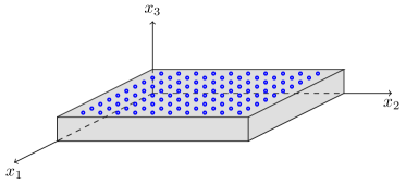
In this problem, is bounded domain with sufficiently smooth boundary , where , , and are mutually disjoint. In 38, is the state variable, is the inversion parameter, and is the secondary uncertain parameter. The Neumann boundary data is , is the unit-length outward normal for the boundaries and , and for simplicity we have considered zero volume source, and homogeneous Dirichlet and Robin conditions. In our numerical experiments, is a three-dimensional domain with a unit square base and height such that aspect ratio (base/height) is 100; see Figure 1. In the present example, is the bottom edge of the domain, is the top edge, and is the union of the side edges. In our computations, we define the boundary source term according to .
Note that in this problem, the inversion and secondary parameters are both functions. The inversion parameter belongs to the Hilbert space , which is equipped with the -inner product. The secondary parameter takes values in . As discussed below, we define as an -valued Gaussian random variable with almost surely continuous realizations, which ensures (almost sure) well-posedness of the problem 38. Below we use and to denote the - and -inner products, respectively. Also, with a slight abuse of notation, we denote the inner-product with as well.
We use measurements of on the top boundary, , to estimate the inversion parameter . The measurements are collected at a set of sensor locations as depicted in Figure 1. Hence, in the present problem, the parameter-to-observable is defined as the composition of a linear observation operator , which extracts solution values at the sensor locations, and the PDE solution operator. Note that this parameter-to-observable map is a nonlinear function of the inversion and secondary parameters.
As detailed in Section 3, we assume a Gaussian noise model, and use the BAE approach to account for the secondary uncertainties in the inverse problem. Also, we use a Gaussian prior law for and model the secondary uncertainty as a Gaussian random variable.777As discussed earlier, the presented framework does not rely on a specific choice of distribution law for . The Gaussian assumption here is merely for computational convenience. For both and , we use covariance operators that are defined as negative powers of Laplacian-like operators [40]; see Section 7. Note that with the appropriate choice of the covariance operator, the realizations of will be almost surely continuous on the closure of .
6.2 OED under uncertainty problem formulation
In this section we discuss the precise definition of , for the model inverse problem discussed in Section 6.1. The MAP estimation problems in 34b require minimizing defined in 21. For notational convenience, in this section, we use the shorthand to denote . In the present example, the first order optimality conditions for this optimization problem are given by
| (39) | |||||
| (40) | |||||
| (41) |
where . For the derivation details, we refer to [33]. Note that 39 is the weak form of the state equation 38, and 40 and 41 are the weak forms of the adjoint and gradient equations, respectively. Note also that the left hand side of 41 describes the action of the derivative of in the direction .
To specify the eigenvalue problem in 34c, we first discuss the action of the operator (evaluated at ) in the direction . In weak form, this Hessian application satisfies,
| (42) |
for every . In 42, for a given , solves the state problem (38), solves the incremental adjoint problem
| (43) |
and solves the so-called incremental state problem
| (44) |
We next summarize the OED problem of minimizing (34) as a PDE-constrained optimization problem specialized for the model inverse problem in Section 6:
| (45a) | |||||
| where, for and , | |||||
| (45b) | |||||
| (45c) | |||||
| (45d) | |||||
| (45e) | |||||
| (45f) | |||||
| (45g) | |||||
| (45h) | |||||
The PDE constraints (45b)–(45d) are the optimality system (39)–(41) characterizing the MAP point described in (34b). The equations (45e)–(45g) are the PDE constraints that describe the Hessian apply and eigenvalue problem. Note that we have reformulated the eigenvalue problem according to 35.
7 Computational results
In this section, we numerically study our OED under uncertainty approach, which we apply to the model inverse problem described in Section 6. We begin by specifying the Bayesian problem setup and discretization details in Section 7.1. Then, we study the impact of secondary model uncertainty on the measurements and compute the BAE error statistics in Section 7.2. Finally, in Section 7.3, we examine the effectiveness of our approach in computing uncertainty aware designs. We also study the impact of ignoring model uncertainty in (i) experimental design stage and (ii) both experimental design and inference stages. Ignoring uncertainty in the design stage amounts to fixing the secondary parameter at its nominal value (i.e., using the approximate model 10) and ignoring the approximation error when solving the OED problem. We refer to designs computed in this manner as uncertainty unaware designs. Note that in the case of (i), the uncertainty is still accounted for when solving the inverse problem. This study illustrates the importance of accounting for model uncertainty, when computing experimental designs. On the other hand, the study of case (ii) illustrates the pitfalls of ignoring uncertainty in both the optimal design problem and subsequent solution of the inverse problem.
7.1 Problem setup
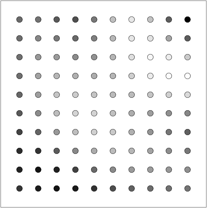
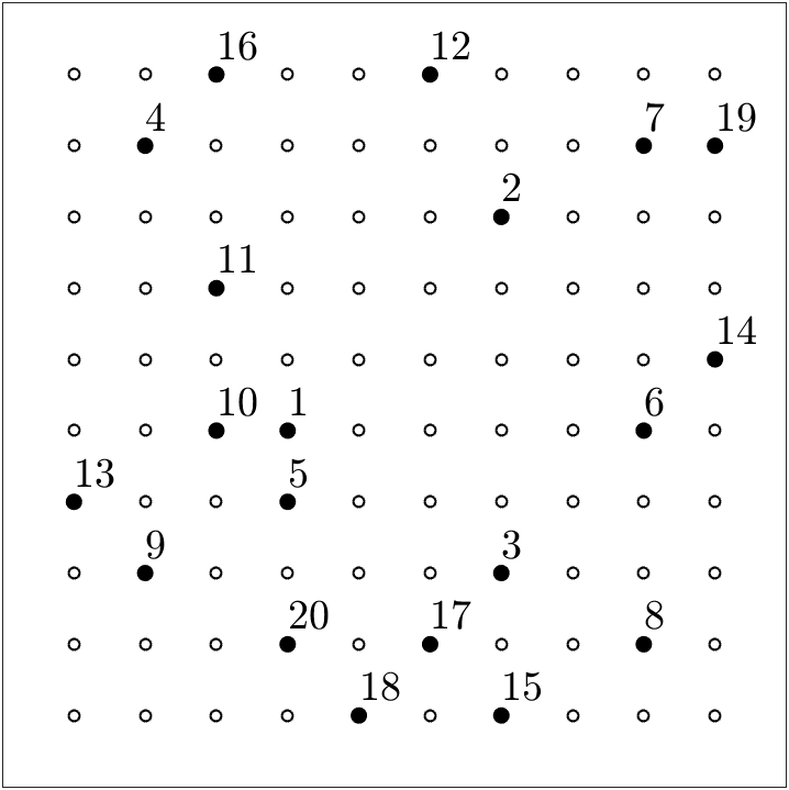
We consider candidate sensor locations that are arranged in a regular grid on the top boundary ; see Figure 1. The additive noise in the synthetic measurements has a covariance matrix of the form , with . This amounts to about one percent noise.
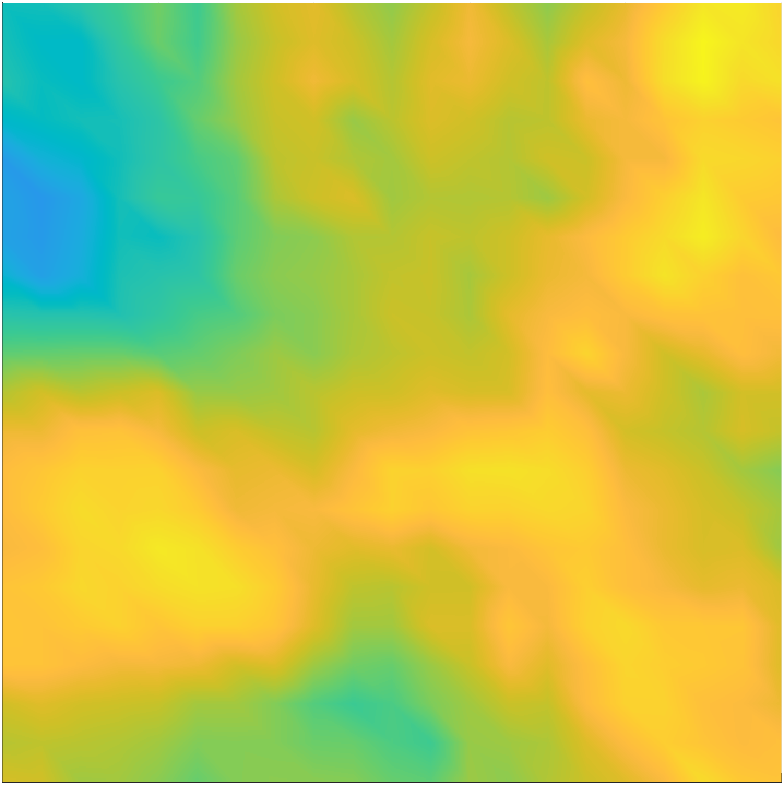
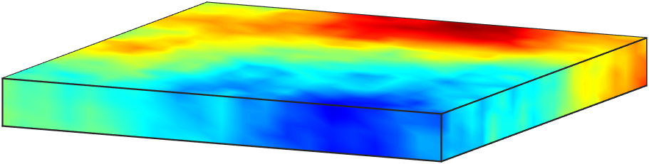
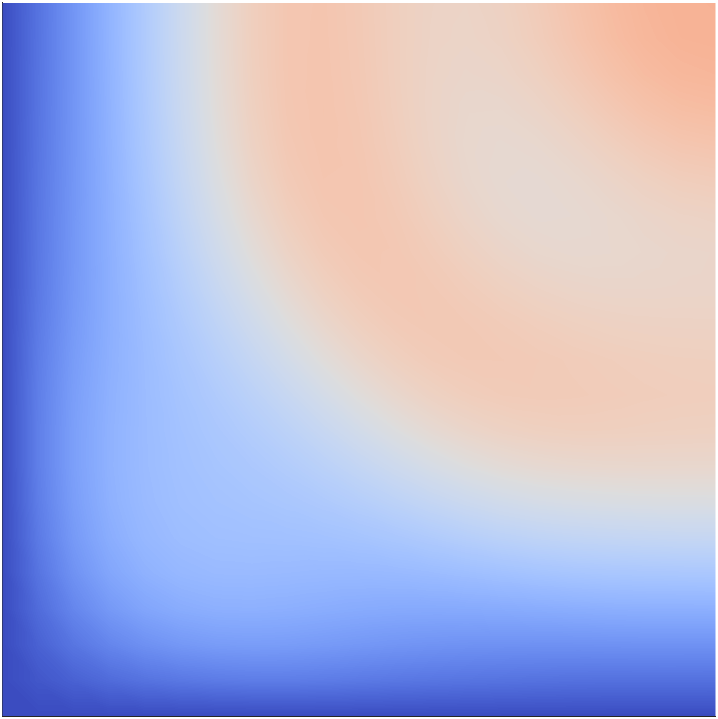
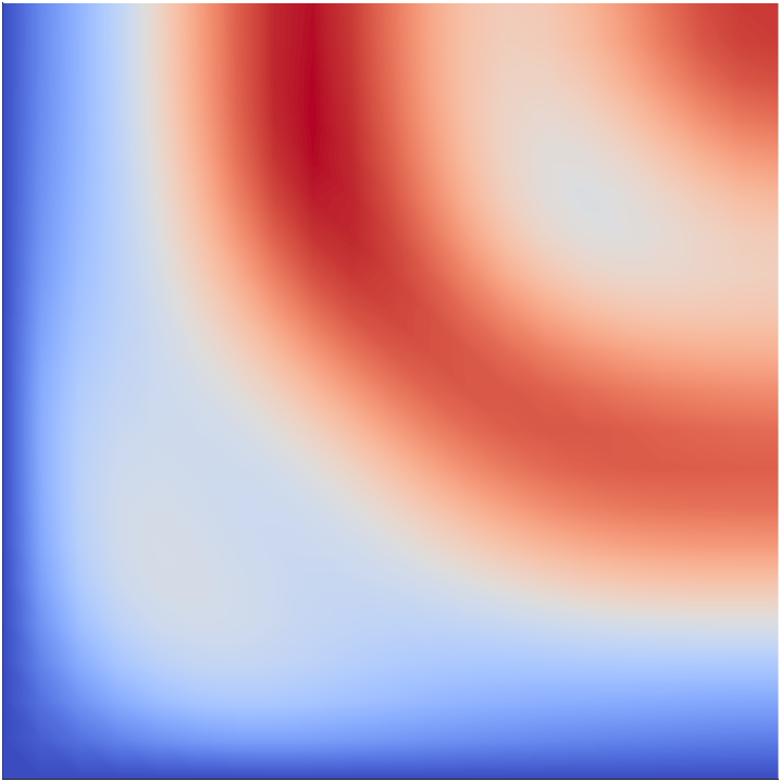
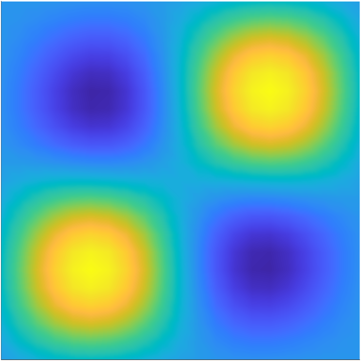
We use a Gaussian prior law for . The prior mean is taken as a constant function , and we use a covariance operator given by the inverse of a Laplacian-like operator. Specifically, we let , with , where we take and . To help mitigate undesirable boundary affects that can arise due to the use of PDE-based prior covariance operators, we equip the operator with Robin boundary conditions [16]. For illustration, four random draws from the prior distribution are shown in Figure 2.
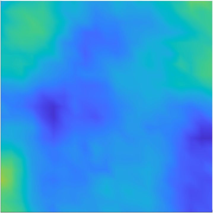
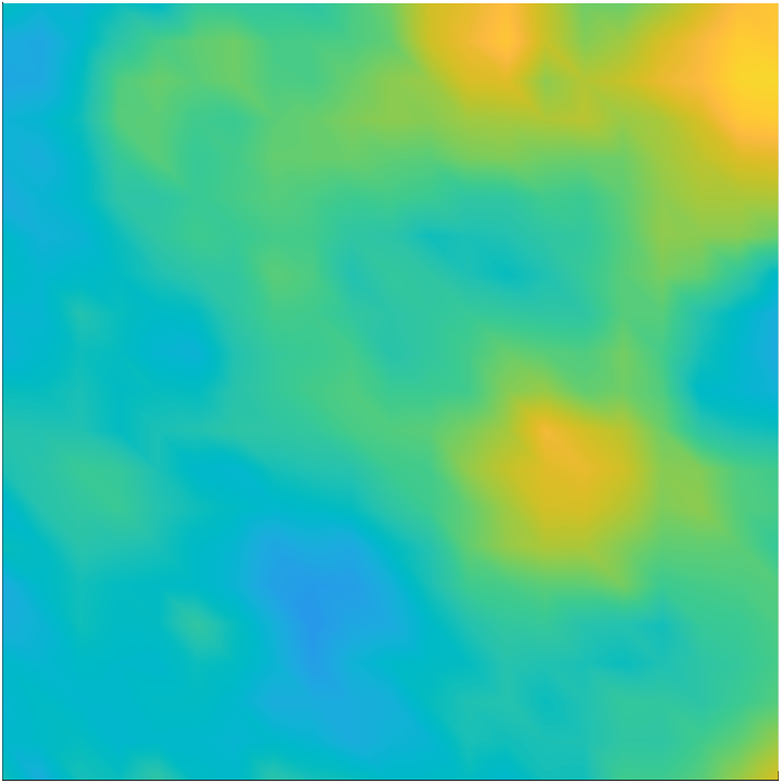
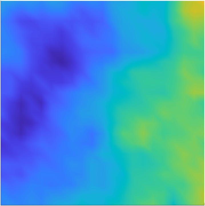
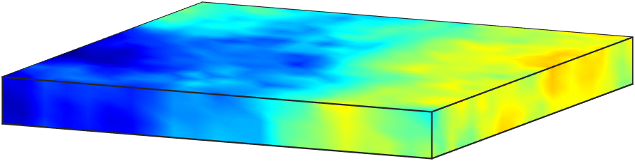
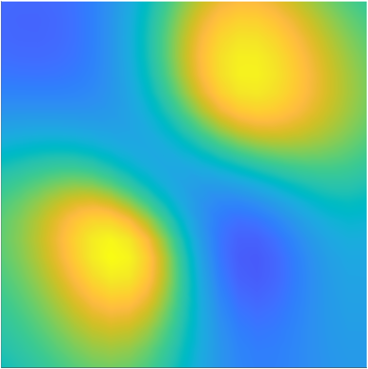
The law of the secondary parameter is chosen to be a Gaussian measure . We set the mean of as the constant function , and the covariance operator is defined as , where with and . This choice of corresponds to a random field with much shorter correlation in the direction than in the - and -directions, inline with aspect ratio of 100 used in defining the domain . We show four representative samples of in Figure 3.

The forward problem 38 is solved using a continuous Galerkin finite element method. We use tetrahedral elements and piecewise linear basis functions. As such, the discretized state and adjoint variables, as well as the secondary parameter , have dimension . On the other hand, the discretized inversion parameter , which is defined on the bottom boundary, is of dimension .
7.2 Incorporating the model uncertainty in the inverse problem
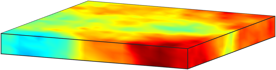
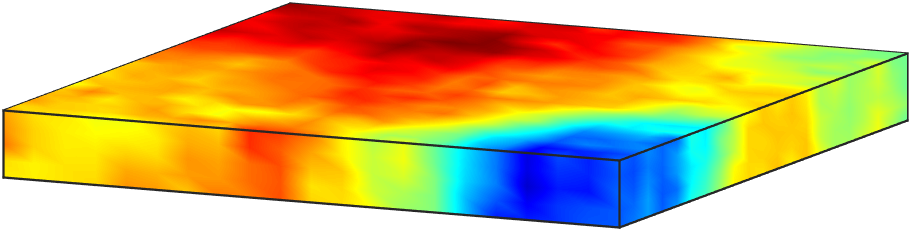
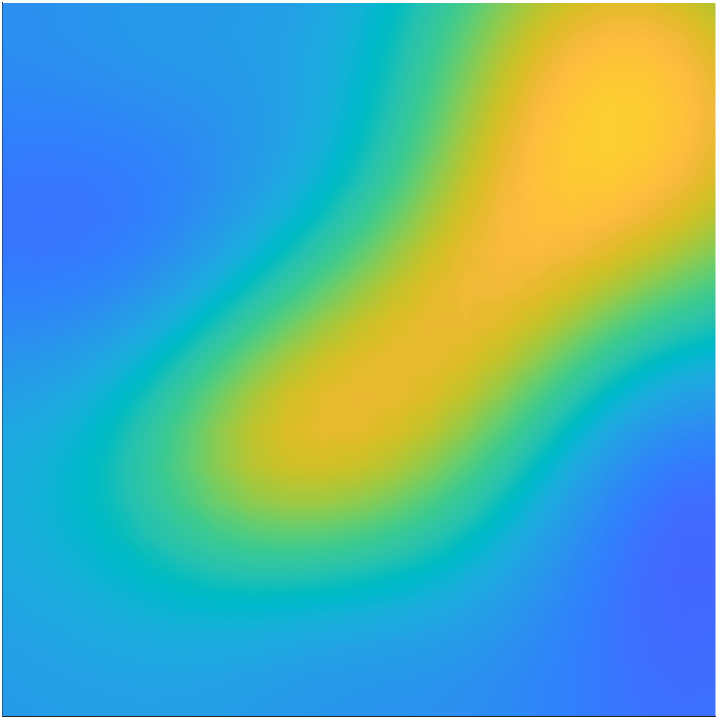
We begin by studying the impact of the secondary parameter on the solution of the forward problem. This is illustrated in Figure 4. In this experiment, we solve the forward problem for a fixed and four different realizations of . Note that, although the qualitative behavior of on is similar for the different samples of , there are considerable differences in the values. This indicates that the approximation error due to fixing at the nominal value will have significant variations.
We compute the sample mean and covariance matrix of the approximation error as in 27 with . The mean and marginal standard deviations are shown in Figure 5. To illustrate the correlation structure of the approximation error, we show the correlation of the approximation error at two of the candidate locations with the other candidate locations in Figure 6 (left-middle). To provide an overall picture, we report the correlation matrix of the approximation error in Figure 6 (right). Note that the approximation errors at the sensor sites are not only larger than the measurement noise, but also they are highly correlated and have a nonzero and non-constant mean. Thus, in the present application, the approximation error due to model uncertainty cannot be ignored and needs to be accounted for.
7.3 Optimal experimental design under uncertainty
We begin by solving the OED problem 45 with training data samples. In Figure 7 (left), we show an uncertainty aware optimal sensor placement with 20 sensors. Note that due to the use of a greedy algorithm, we can track the order in which the sensors are picked. To understand the impact of ignoring model uncertainty in the design stage, we also compute an uncertainty unaware design; this is reported in Figure 7 (right).
To evaluate the quality of the computed designs, we first study the expected posterior variance and expected relative error of the MAP point. To facilitate this, we draw parameter samples from and generate validation data samples,
where and are draws from and , respectively. Then, we consider
| (46) |
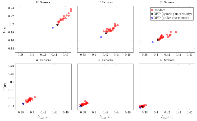
In our numerical experiments we use . We compare and when solving the inverse problem with the computed optimal design versus randomly chosen designs in Figure 8, where we consider designs with different numbers of sensors. We also examine the impact of ignoring the model uncertainty in solving the OED problem (see the black dots in Figure 8). Note that the uncertainty aware designs outperform the random designs as well as the uncertainty unaware designs. This is most pronounced when the number of sensors is small. This is precisely when optimal placement of sensors is crucial. We also observe that as the number of sensors in the designs increase, the cloud moves left and downward. This is expected. The more sensors we use, the more we can improve the quality of the MAP point and reduce posterior uncertainty. For , we note that the difference between uncertainty aware and uncertainty unaware designs become small (in the case of , they nearly overlap). For , even the random designs become competitive. All these are expected. As mentioned, earlier, optimal placement of sensors is crucial, when we have access only to a “small” number measurement points. What constitutes “small” is problem dependent.
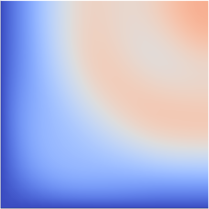
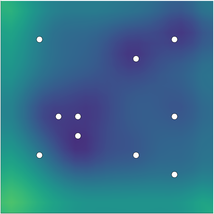
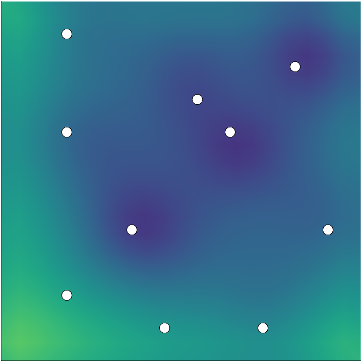
Next, we illustrate the effectiveness of the computed optimal designs in reducing posterior uncertainty. To this end, we consider the computed optimal designs with 10 sensors. In Figure 9, we show the effectiveness of the uncertainty aware optimal design in reducing posterior uncertainty; we also report the posterior standard deviation field, when solving the inverse problem with an uncertainty unaware design. To complement this study, we consider the quality of the MAP points computed using uncertainty aware and uncertainty unaware designs in Figure 10. Overall, we observe that the uncertainty aware design is more effective in reducing posterior uncertainty and results in a higher quality MAP point. This conclusion is also supported by the results reported in Figure 8.
Note that the data used to solve the inverse problem is synthesized by solving the PDE model 1, using our choice of the “truth” inversion parameter (see Figure 10 (left)) and a randomly chosen followed by extracting measurements at the sensor sites and adding measurement noise. This simulates the practical situation when field data that corresponds to an unknown choice of is collected.


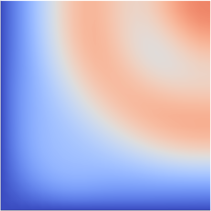
In the above experiments, when examining the performance of uncertainty unaware designs, model uncertainty was still accounted for (following the BAE framework) when solving the inverse problem using these designs. Next, we examine the impact of ignoring model uncertainty in both OED and inference stages. For this experiment, we use the same synthesized data as that used to obtain the results in Figure 10 (right). In Figure 11 we report the result of solving the inverse problem with an uncertainty unaware design, when ignoring model uncertainty in the inverse problem as well. We note an impressive reduction of uncertainty; see Figure 11 (left), which uses the same scale as the standard deviation plots in Figure 9. On the other hand, the MAP point computed in this case is of very poor quality; see Figure 11 (right), where we have used the same scale as the MAP point plots in Figure 10. Intuitively, this indicates that ignoring model uncertainty in both OED and inference stages, in presence of significant modeling uncertainties, can lead to an unfortunate situation where one is highly certain (i.e., low posterior variance) about a very wrong parameter estimate.
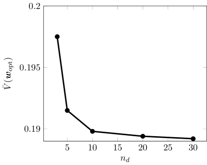
As mentioned earlier, we used training data samples when solving the OED problem 45. Clearly, increasing would improve the quality of the design—we would be optimizing a more accurate estimate of the OED objective. However, this comes with increased computational overhead. In practice, typically a small is effective in obtaining good quality designs. This is demonstrated in the results above (e.g., fig. 8). To examine the impact of changing on the quality of the computed optimal design, we perform a brief computational study where we focus on designs with 10 sensors. We compute the expected value of the posterior variance (as in 46) at the computed optimal design, , with values of . The results are reported in fig. 12. As before, is computed with validation data samples. Note that going beyond results in diminishing returns. This, however, entails increased computational cost. In practice, studies such as the one conducted here may be necessary to estimate a reasonable choice for . In the present example, we see that is approximately at the “elbow” of the curve in fig. 12, making it a reasonable practical choice.
8 Conclusions
In the present work, we addressed OED under uncertainty for Bayesian nonlinear inverse problems governed by PDEs with infinite-dimensional inversion and secondary parameters. We have presented a mathematical framework and scalable computational methods for computing uncertainty aware optimal designs. Our results demonstrate that ignoring the uncertainty in the OED and/or the parameter inversion stages can lead to inferior designs and inaccurate parameter estimation. Hence, it is important to account for modeling uncertainties in Bayesian inversion and OED.
The limitations of the proposed approach are in its reliance on Gaussian approximations for the posterior and the approximation error. The former is a common approach in large-scale Bayesian inverse problems as well as in the BAE literature. The Gaussian approximation to the posterior is suitable if a linearization of the forward model, at the MAP point, is sufficiently accurate for the set of parameters with significant posterior probability. On the other hand, the Gaussian approximation of the approximation error, which is guided by the BAE approach, might fail to adequately capture the distribution of the approximation error. However, as shown in various studies in the BAE literature, this Gaussian approximation is reasonable in broad classes of inverse problems; see, e.g., [27, 24, 32, 33]. Additionally, in the present work we considered a greedy approach for tackling the binary OED optimization problems. This can become expensive if the number of candidate sensor locations or the desired number of sensors in the computed sensor placements become very large.
The numerical experiments in the present work focus on an academic, albeit application-driven, model problem. The present application was chosen since it exhibits key problem structures seen in broad classes of ill-posed inverse problems. Namely, smoothing properties of the forward operator lead to low-rank structures that can be exploited when developing numerical methods. The present numerical study also builds on and complements the previous study of BAE for the Robin boundary condition inversion problems in [33]. Examining the properties of the present method in more challenging inverse problems with multiple types of modeling uncertainties is a subject for future work.
The discussions in this article point to a number of opportunities for future work. In the first place, we point out that the use of BAE approach to account for modeling uncertainties in Bayesian inverse problems is only one possible application of this approach. In general, BAE has been used in a wide range of applications to account for uncertainty due to the use of approximate forward models. For example, BAE can be used to model the approximation errors due to the use of reduced order models or upscaled models. BAE has also been used to account for the errors due to the use of a mean-field model instead of an underlying high-fidelity stochastic model [38]. Thus, the framework presented for OED under uncertainty in the present work can be extended to OED in inverse problems where the forward model is replaced with a low-fidelity approximate model instead of a computationally intensive high-fidelity model, as long the approximation error can be modeled adequately by a Gaussian.
Another interesting line of inquiry involves replacing the greedy strategy used to find optimal designs with more powerful optimization algorithms. One possibility is to follow a relaxation approach [31, 3, 4, 8] where the design weights are allowed to take values in the interval . This enables use of efficient gradient-based optimization algorithms and can be combined with a suitable penalty approach to control the sparsity of the computed sensor placements. An attractive alternative is the approach in [9], which tackles the binary OED optimization problem by replacing it with a related stochastic programming problem. A further line of inquiry is investigating the idea of using fixed MAP points, computed prior to solving the OED problem, as done in [44] for OED problems with no additional uncertainties. This idea, at the expense of further approximations, replaces the bilevel optimization problem with a simpler one, hence reducing computational cost significantly.
Finally, in inverse problems governed by complex models with multiple sources of secondary uncertainty, an a priori sensitivity analysis of the Bayesian inverse problem may be necessary to identify secondary modeling uncertainties that are most influential to the solution of the inverse problem. This may be accomplished by suitable adaptations of hyper-differential sensitivity analysis methods for inverse problems [42, 36, 41].
References
References
- [1] A. Alexanderian. Optimal experimental design for infinite-dimensional Bayesian inverse problems governed by PDEs: A review. Inverse Problems, 37(4), 2021.
- [2] A. Alexanderian, P. J. Gloor, and O. Ghattas. On Bayesian A-and D-optimal experimental designs in infinite dimensions. Bayesian Anal., 11(3):671–695, 2016.
- [3] A. Alexanderian, N. Petra, G. Stadler, and O. Ghattas. A-optimal design of experiments for infinite-dimensional Bayesian linear inverse problems with regularized -sparsification. SIAM J. Sci. Comput., 36(5):A2122–A2148, 2014.
- [4] A. Alexanderian, N. Petra, G. Stadler, and O. Ghattas. A fast and scalable method for A-optimal design of experiments for infinite-dimensional Bayesian nonlinear inverse problems. SIAM J. Sci. Comput., 38(1):A243–A272, 2016.
- [5] A. Alexanderian, N. Petra, G. Stadler, and I. Sunseri. Optimal design of large-scale Bayesian linear inverse problems under reducible model uncertainty: good to know what you don’t know. SIAM/ASA J. Uncertain. Quantif., 9(1):163–184, 2021.
- [6] A. Y. Aravkin and T. Van Leeuwen. Estimating nuisance parameters in inverse problems. Inverse Problems, 28(11):115016, 2012.
- [7] A. C. Atkinson and A. N. Donev. Optimum Experimental Designs. Oxford, 1992.
- [8] A. Attia and E. Constantinescu. Optimal experimental design for inverse problems in the presence of observation correlations. SIAM J. Sci. Comput., 44(4):A2808–A2842, 2022.
- [9] A. Attia, S. Leyffer, and T. S. Munson. Stochastic learning approach for binary optimization: Application to Bayesian optimal design of experiments. SIAM J. Sci. Comput., 44(2):B395–B427, 2022.
- [10] O. Babaniyi, R. Nicholson, U. Villa, and N. Petra. Inferring the basal sliding coefficient field for the Stokes ice sheet model under rheological uncertainty. The Cryosphere, 15(4):1731–1750, 2021.
- [11] A. Bartuska, L. Espath, and R. Tempone. Small-noise approximation for Bayesian optimal experimental design with nuisance uncertainty. Comput. Methods Appl. Mech. Engrg., 399:115320, 2022.
- [12] T. Bui-Thanh, O. Ghattas, J. Martin, and G. Stadler. A computational framework for infinite-dimensional Bayesian inverse problems. Part I: The linearized case, with application to global seismic inversion. SIAM J. Sci. Comput., 35(6):A2494–A2523, 2013.
- [13] K. Chaloner and I. Verdinelli. Bayesian experimental design: A review. Statist. Sci., 10(3):273–304, 1995.
- [14] E. M. Constantinescu, N. Petra, J. Bessac, and C. G. Petra. Statistical treatment of inverse problems constrained by differential equations-based models with stochastic terms. SIAM/ASA J. Uncertain. Quantif., 8(1):170–197, 2020.
- [15] G. Da Prato. An introduction to infinite-dimensional analysis. Springer, 2006.
- [16] Y. Daon and G. Stadler. Mitigating the influence of boundary conditions on covariance operators derived from elliptic PDEs. Inverse Probl. Imaging, 12(5):1083–1102, 2018.
- [17] M. Dashti and A. M. Stuart. The Bayesian approach to inverse problems. In R. Ghanem, D. Higdon, and H. Owhadi, editors, Handbook of Uncertainty Quantification, pages 311–428. Spinger, 2017.
- [18] C. Feng and Y. M. Marzouk. A layered multiple importance sampling scheme for focused optimal Bayesian experimental design. preprint, 2019. https://arxiv.org/abs/1903.11187.
- [19] G. H. Golub and C. F. Van Loan. Matrix computations. Johns Hopkins Studies in the Mathematical Sciences. Johns Hopkins University Press, Baltimore, MD, fourth edition, 2013.
- [20] E. Haber, L. Horesh, and L. Tenorio. Numerical methods for experimental design of large-scale linear ill-posed inverse problems. Inverse Problems, 24(055012):125–137, 2008.
- [21] N. Halko, P.-G. Martinsson, and J. A. Tropp. Finding structure with randomness: Probabilistic algorithms for constructing approximate matrix decompositions. SIAM Rev., 53(2):217–288, 2011.
- [22] T. Isaac, N. Petra, G. Stadler, and O. Ghattas. Scalable and efficient algorithms for the propagation of uncertainty from data through inference to prediction for large-scale problems, with application to flow of the Antarctic ice sheet. J. Comput. Phys., 296:348–368, 2015.
- [23] J. Jagalur-Mohan and Y. M. Marzouk. Batch greedy maximization of non-submodular functions: Guarantees and applications to experimental design. J. Mach. Learn. Res., 22, 2021.
- [24] J. Kaipio and V. Kolehmainen. Approximate marginalization over modeling errors and uncertainties in inverse problems. Bayesian Theory and Applications, pages 644–672, 2013.
- [25] J. Kaipio and E. Somersalo. Statistical and Computational Inverse Problems, volume 160 of Applied Mathematical Sciences. Springer-Verlag, New York, 2005.
- [26] J. Kaipio and E. Somersalo. Statistical inverse problems: discretization, model reduction and inverse crimes. Journal of computational and applied mathematics, 198(2):493–504, 2007.
- [27] V. Kolehmainen, T. Tarvainen, S. R. Arridge, and J. P. Kaipio. Marginalization of uninteresting distributed parameters in inverse problems-application to diffuse optical tomography. Int. J. Uncertain. Quantif., 1(1), 2011.
- [28] K. Koval, A. Alexanderian, and G. Stadler. Optimal experimental design under irreducible uncertainty for linear inverse problems governed by PDEs. Inverse Problems, 36(7), 2020.
- [29] A. Krause, A. Singh, and C. Guestrin. Near-optimal sensor placements in Gaussian processes: Theory, efficient algorithms and empirical studies. J. Mach. Learn. Res., 9:235–284, 2008.
- [30] F. Li. A combinatorial approach to goal-oriented optimal Bayesian experimental design. Master’s thesis, Massachusetts Institute of Technology, 2019.
- [31] S. Liu, S. P. Chepuri, M. Fardad, E. Maşazade, G. Leus, and P. K. Varshney. Sensor selection for estimation with correlated measurement noise. IEEE Trans. Signal Process., 64(13):3509–3522, 2016.
- [32] M. Mozumder, T. Tarvainen, S. Arridge, J. P. Kaipio, C. D’Andrea, and V. Kolehmainen. Approximate marginalization of absorption and scattering in fluorescence diffuse optical tomography. Inverse Problems & Imaging, 10(1):227, 2016.
- [33] R. Nicholson, N. Petra, and J. P. Kaipio. Estimation of the Robin coefficient field in a Poisson problem with uncertain conductivity field. Inverse Problems, 34(11):115005, 2018.
- [34] R. Nicholson, N. Petra, U. Villa, and J. P. Kaipio. On global normal linear approximations for nonlinear Bayesian inverse problems. Inverse Problems, 39(5):054001, 2023.
- [35] F. J. Pinski, G. Simpson, A. M. Stuart, and H. Weber. Kullback–Leibler approximation for probability measures on infinite dimensional spaces. SIAM J. Math. Anal., 47(6):4091–4122, 2015.
- [36] W. Reese, J. Hart, B. van Bloemen Waanders, M. Perego, J. Jakeman, and A. Saibaba. Hyper-differential sensitivity analysis in the context of Bayesian inference applied to ice-sheet problems. International Journal for Uncertainty Quantification, 14(3).
- [37] G. Shulkind, L. Horesh, and H. Avron. Experimental design for nonparametric correction of misspecified dynamical models. SIAM/ASA J. Uncertain. Quantif., 6(2):880–906, 2018.
- [38] M. J. Simpson, R. E. Baker, P. R. Buenzli, R. Nicholson, and O. J. Maclaren. Reliable and efficient parameter estimation using approximate continuum limit descriptions of stochastic models. J. Theoret. Biol., 549, 2022.
- [39] R. C. Smith. Uncertainty quantification: Theory, implementation, and applications, volume 12 of Computational Science and Engineering Series. SIAM, 2013.
- [40] A. M. Stuart. Inverse problems: A Bayesian perspective. Acta Numerica, 19:451–559, 2010.
- [41] I. Sunseri, A. Alexanderian, J. Hart, and B. van Bloemen Waanders. Hyper-differential sensitivity analysis for nonlinear Bayesian inverse problems. International Journal for Uncertainty Quantification, 14(2), 2024.
- [42] I. Sunseri, J. Hart, B. van Bloemen Waanders, and A. Alexanderian. Hyper-differential sensitivity analysis for inverse problems constrained by partial differential equations. Inverse Problems, 2020.
- [43] D. Uciński. Optimal measurement methods for distributed parameter system identification. CRC Press, Boca Raton, 2005.
- [44] K. Wu, P. Chen, and O. Ghattas. A fast and scalable computational framework for large-scale high-dimensional Bayesian optimal experimental design. SIAM/ASA Journal on Uncertainty Quantification, 11(1):235–261, 2023.