Optimal execution of equity with geometric price process

Gerardo Hernandez-del-Valle Statistics Department, Columbia University
1255 Amsterdam Ave. Room 1005, New York, N.Y., 10027. gerardo@stat.columbia.edu and Carlos G. Pacheco-Gonzalez Mathematics Department, CINVESTAV-IPN
Av. Instituto Polit cnico Nacional #2508, Col. San Pedro Zacatenco, México, D.F., C.P. 07360 cpacheco@math.cinvestav.mx

(Date: October 14, 2009)

Abstract.

In this paper we derive the Markowitz-optimal, deterministic-execution trajectory for a trader who wishes to buy or sell a large position of a share which evolves as a geometric Brownian motion in contrast to the arithmetic model which prevails in the existing literature. Our calculations include a general temporary impact, rather than a specific function. Additionally, we point out—under our setting—what are the necessary ingredients to tackle the problem with adaptive execution trajectories. We provide a couple of examples which illustrate the results. We would like to stress the fact that in this paper we use understandable user-friendly techniques.

2000 Mathematics Subject Classification:

Primary: 91B28, 49K15

The research of this author was partially supported by Algorithmic Trading Management LLC

1. Introduction

The problem of optimal execution is a very general problem in which a trader who wishes to buy or sell a large position $K$ of a given asset $S$ —for instance wheat, shares, derivatives, etc.—is confronted with the dilemma of executing slowly or as quick as possible. In the first case he/she would be exposed to volatility, and in the second to the laws of offer and demand. Thus the trader most hedge between the market impact (due to his trade) and the volatility (due to the market).

The key ingredients to study this optimization problem are: (1) The modeling of the asset—which is typically modeled as a geometric Brownian process. (2) The modeling of the so-called market impact which heuristically suggests the existence of an instantaneous impact—so-called temporary—and a cumulative component referred to as permanent. And finally (3) one should establish a criteria of optimality.

The main aim of this paper is to study and characterize the so-called Markowitz-optimal open-loop execution trajectory, in terms of nonlinear second order, ordinary differential equations (Theorems 3.2 and 3.6). The above is done for a trader who wishes to buy or sell a large position $K$ of shares $S$ which evolve as a geometric Brownian motion (although in the existing literature it is considered an arithmetic Brownian motion for this problem). In this paper we only deal with deterministic strategies, also called open loop controls; however, we point out—in Section 5—the key ingredients to address the problem with adaptive strategies, also termed Markovian controls (work in progress).

The main motivation of this work is on one hand economic, but on the other the effect of market impact in the valuation of contingent claims, and its connection with optimal execution of derivatives. Intuitively, for this kind of problem, one would expect to consider adaptive strategies to tackle the questions, although it seems natural to first understand the deterministic case. An important element in our analysis, will be the use of a linear stochastic differential equation, first used—to our knowledge—by Brennan and Schwartz (1980) in their study of interest rates.

The problem of minimizing expected overall liquidity costs has been analyzed using different market models by Bertsimas and Lo (1998), Obizhaeva and Wang, and Alfonsi et al. (2007a,2007b), just to mention a few. However, these approaches miss the volatility risk associated with time delay. Instead, Almgren and Chriss (1999,2000), suggested studying and solving a mean-variance optimization for sales revenues in the class of deterministic strategies. Further, on Almgren and Lorenz (2007) allowed for intertemporal updating and proved that this can strictly improve the mean-variance performance. Nevertheless, in Schied and Schöneborn (2007), the authors study the original problem of expected utility maximization with CARA utility functions. Their main result states that for CARA investors there is surprisingly no added utility from allowing for intertemporal updating of strategies. Finally, we mention that the Hamilton-Jacobi-Bellman approach has also recently been studied in Forsyth (2009).

Our paper is organized as follows: In Section 2 we introduce our model, assumptions and auxiliary results. Namely through a couple of subsequent Propositions we characterize and compute—by use of a Brennan-Schwartz type process (3)—the moments of certain random variable that is relevant in our optimization problem. Section 3 is devoted to deriving and proving the characterization of our optimal trading strategies and the optimal value function as well. After that, in Section 4, we present a couple of examples in order to exemplify the procedure derived in Section 3. We first compare Almgren and Chriss trajectory with ours, and in Example 2 we use a temporary market impact $h$ to the power $3/5$ as suggested in the empirical study of Almgren et. al.’s (2005). We conclude the paper, in Section 5, by pointing out the key ingredients in the study of adaptive execution strategies.

2. Auxiliary Results

In this section, we describe the dynamics of the asset $S$ , the so-called market impact, and we introduce the Brennan-Schwartz process. This process will allow us not only to compute the moments of the optimization argument, but also to represent it in terms of an SDE. For the remainder of this section, let $c(t)$ be a fixed and differentiable function for $0\leq t\leq T<\infty$ .

2.1. The model.

Let the price of the share $S$ of a given company evolve as a geometric process, where the random component $B$ is standard Brownian motion, i.e.

\displaystyle dS_{t}

\displaystyle=

\displaystyle S_{t}\left[\left(g(c(t))+\frac{dh(c(t))}{dt}\right)dt+\sigma dB_{t}\right],\qquad S_{0}=s,

and where $g$ and $h$ represent respectively the permanent—which accumulates over time—and instantaneous temporary impact. Thus, the future effective price per share due to our trade can be modelled as

(1)

\displaystyle S_{t}=s\exp\left\{\int_{0}^{u}g(c(v))dv+h(c(u))-\frac{1}{2}\sigma^{2}u+\sigma B_{u}\right\},

where $\sigma>0$ is an estimable parameter.

Remark 2.1.

(a) Note that that process $\ln(S)$ , where $S$ is as in (1), coincides precisely with the “standard” notion of both permanent and temporary impact. That is, if we model the price process as arithmetic Brownian motion:

\displaystyle dS_{t}=\sigma dB_{t}+g(c(t))dt+\frac{dh}{dt}(c(t)),\qquad S_{0}=s

then

\displaystyle S_{t}-s=\int_{0}^{t}g(c(u))du+h(c(t))+\sigma B_{t}.

Hence, the first term in the right-hand side of the equality is accumulating over time, on the other hand, the second term is not.
(b) Next, observe that the process $c$ can be thought of as a control, which in turn may be:

(1)

an admissible process $c$ which is adapted to the natural filtration $\mathcal{F}^{S}$ of the associated process (1) is called a feedback control,
(2)

an admissible process $c$ which can be written in the form $c_{t}=u(t,S_{t})$ for some measurable map $u$ is called Markovian control, notice that any Markovian control is a feedback control,
(3)

a deterministic processes of the family of admissible controls are called open loop controls.

(c) In this paper we will only deal with open loop controls, yet to study feedback controls it will become quite useful to introduce the so-called Brennan-Schwartz process, introduced in the next subsection. The reason being, that to derive the Hamilton-Jacobi-Bellman equation—see Section 5—it is more convenient to have a diffusion instead of an average of a diffusion.

2.2. Averaged geometric and Brennan-Schwartz processes

In order to study our problem we will introduce the following averaged geometric Brownian process:

(2)

\displaystyle\xi_{t}

\displaystyle:=

\displaystyle\int_{0}^{t}c(u)S_{u}du,\qquad t\geq 0.

By (1) we can express $\xi_{t}$ as

\displaystyle\xi_{t}

\displaystyle=

\displaystyle\int_{0}^{t}c(u)se^{\int_{0}^{u}g(c(v))dv+h(c(u))-\frac{1}{2}\sigma^{2}u+\sigma B_{u}}du.

Thus, if $c(u)$ represents the number of shares bought or sold at time $u$ at price $S_{u}$ , then $\xi_{t}$ represents the total amount spent or earned by the trader up to time $t$ .

To compute the moments of $\xi$ we will use the following linear non-homogeneous stochastic differential equation

(3)		$\displaystyle dX_{t}$	$\displaystyle=$	$\displaystyle\left[c(t)-\left(g(c(t))+\frac{dh(c(t))}{dt}-\sigma^{2}\right)X_{t}\right]dt-\sigma X_{t}dB_{t}$
	$\displaystyle X_{0}$	$\displaystyle=$	$\displaystyle 0,$

which has been used for instance by Brennan and Schwartz (1980) in the modeling of interest rates, by Kawaguchi and Morimoto (2007) in environmental economics, and which may also be used to study the density of averaged geometric Brownian motion [see for instance, Linetsky (2004)].

In general, its usefulness is due to the fact that one may construct a Brennan-Schwartz process $X$ which satisfies

X\stackrel{{\scriptstyle\mathcal{D}}}{{=}}\xi,

where $\stackrel{{\scriptstyle\mathcal{D}}}{{=}}$ stands for equality in distribution. In this paper, it is used, together with Itô’s lemma to show that $\xi=S\cdot X$ , which alternatively will allow us to compute the second moment of $\xi$ in terms of an iterated integral, indeed:

Proposition 2.2.

Let processes $S$ , $\xi$ , and $X$ be as in (1), (2), and (3), respectively, then

\displaystyle\xi_{t}=S_{t}\cdot X_{t},\qquad t\geq 0

and

\displaystyle d\xi^{2}_{t}=2\xi_{t}S_{t}c(t)dt.

Proof.

By Itô’s lemma

$\displaystyle d(S_{t}\cdot X_{t})$	$\displaystyle=$	$\displaystyle S_{t}dX_{t}+X_{t}dS_{t}+dX_{t}dS_{t}$
	$\displaystyle=$	$\displaystyle S_{t}c(t)dt-S_{t}X_{t}\left(g(c(t))+\frac{dh(c(t))}{dt}\right)dt+S_{t}X_{t}\sigma^{2}dt$
		$\displaystyle-\sigma S_{t}X_{t}dB_{t}+X_{t}S_{t}\left(g(c(t))+\frac{dh(c(t))}{dt}\right)dt$
		$\displaystyle+\sigma X_{t}S_{t}dB_{t}-\sigma^{2}S_{t}X_{t}dt$
	$\displaystyle=$	$\displaystyle c(t)S_{t}dt$
	$\displaystyle=$	$\displaystyle\xi_{t}.$

Furthermore, for the second moment of $\xi$ it follows that

$\displaystyle d\xi^{2}_{t}$	$\displaystyle=$	$\displaystyle 2X_{t}S^{2}_{t}dX_{t}+2X^{2}_{t}S_{t}dS_{t}+S^{2}_{t}(dX_{t})^{2}+X^{2}_{t}(dS_{t})^{2}$
		$\displaystyle+4X_{t}S_{t}(dX_{t}\cdot dS_{t})$
	$\displaystyle=$	$\displaystyle 2X_{t}S^{2}_{t}sc(t)dt-2X_{t}S^{2}_{t}\left(g(c(t))+\frac{dh(c(t))}{dt}\right)X_{t}dt$
		$\displaystyle+2X_{t}S^{2}_{t}\sigma^{2}X_{t}dt-2X_{t}S^{2}_{t}\sigma X_{t}dB_{t}$
		$\displaystyle+2X^{2}_{t}S_{t}\left(g(c(t))+\frac{dh(c(t))}{dt}\right)S_{t}dt+2X^{2}_{t}S_{t}\sigma S_{t}dB_{t}$
		$\displaystyle+S^{2}_{t}\sigma^{2}X^{2}_{t}dt+X^{2}_{t}\sigma^{2}S^{2}_{t}dt-4X_{t}S_{t}\sigma^{2}X_{t}S_{t}dt$
	$\displaystyle=$	$\displaystyle 2X_{t}S^{2}_{t}c(t)dt$
	$\displaystyle=$	$\displaystyle 2\xi_{t}S_{t}c(t)dt,$

as claimed. ∎

Remark 2.3.

The previous proposition may be derived directly from the integration by parts formula. Yet, this characterization will be useful in the study, for instance, of the optimal trading schedule of derivatives or in the determination of Markovian controls.

2.3. Moments of $\xi$

Now, by Proposition 2.2, it is straightforward to compute the first two moments of $\xi_{t}$ which will be used to solve our optimal execution problem.

Corollary 2.4.

Let $\xi$ be as in (2). Then

(4)		$\displaystyle\mathbb{E}[\xi_{t}]$	$\displaystyle=$	$\displaystyle\int_{0}^{t}c(u)s\exp\left\{\int_{0}^{u}g(c(v))dv+h(c(u))\right\}du$
	$\displaystyle\mathbb{E}[\xi^{2}_{t}]$	$\displaystyle=$	$\displaystyle 2\int_{0}^{t}c(u)se^{\int_{0}^{u}g(c(n))dn+h(c(u))}$
			$\displaystyle\quad\times\left(\int_{0}^{u}c(v)se^{\int_{0}^{v}g(c(w))dw+h(c(v))+\sigma^{2}v}dv\right)du.$

Proof.

By (2):

	$\displaystyle\mathbb{E}[\xi_{t}]$	$\displaystyle=$	$\displaystyle\int_{0}^{t}c(u)s\mathbb{E}[S_{u}]du$
		$\displaystyle=$	$\displaystyle\int_{0}^{t}c(u)s\exp\left\{\int_{0}^{u}g(c(v))dv+h(c(u))\right\}du.$

From Proposition 2.2:

$\displaystyle\mathbb{E}[\xi^{2}_{t}]$	$\displaystyle=$	$\displaystyle 2\mathbb{E}\left[\int_{0}^{t}c(u)sS_{u}\xi_{u}du\right]$
	$\displaystyle=$	$\displaystyle 2\mathbb{E}\left[\int_{0}^{t}c(u)s^{2}S_{u}\left(\int_{0}^{u}c(v)sS_{v}dv\right)du\right]$
	$\displaystyle=$	$\displaystyle 2\int_{0}^{t}c(u)s^{2}\left(\int_{0}^{u}c(v)s\mathbb{E}[S_{u}S_{v}]dv\right)du.$

Therefore, since

$\displaystyle\mathbb{E}\left[e^{\sigma B_{u}+\sigma B_{v}}\right]$	$\displaystyle=$	$\displaystyle\mathbb{E}\left[e^{\sigma(B_{u}-B_{v})+2\sigma B_{v}}\right]$
	$\displaystyle=$	$\displaystyle\mathbb{E}\left[e^{\sigma(B_{u}-B_{v})}\right]\mathbb{E}\left[e^{2\sigma B_{v}}\right]$
	$\displaystyle=$	$\displaystyle e^{\frac{1}{2}\sigma^{2}(u-v)}e^{2\sigma^{2}v},$

it follows that

	$\displaystyle\mathbb{E}[\xi^{2}_{t}]$	$\displaystyle=$	$\displaystyle 2\int_{0}^{t}c(u)se^{\int_{0}^{u}g(c(n))dn+h(c(u))}$
			$\displaystyle\quad\times\left(\int_{0}^{u}c(v)se^{\int_{0}^{v}g(c(w))dw+h(c(v))+\sigma^{2}v}dv\right)du.$

∎

3. Markowitz Optimal open-loop Trading trajectory

In this section we derive a Markowitz-optimal open-loop trading strategy, Theorem 3.2 and 3.6, employing the auxiliary results derived in the previous section.

3.1. Execution shortfall

If the size of the trade $K$ is “relatively” small we would expect the market impact to be negligible, that is, the trader should execute $K$ immediately. Thus, it seems natural to compare the actual total gains (losses) $\xi_{T}$ with the impact-free quantity $Ks$ by introducing the so-called execution shortfall $Y$ defined as

(6)

\displaystyle Y:=\xi_{T}-Ks.

If we use Markowitz optimization criterion, then our problem is equivalent to finding the trading trajectory $\{c(t)|0\leq t\leq T\}$ which minimizes simultaneously the expected shortfall given a fixed risk-aversion level $\lambda$ characterized by the volatility of $Y$ :

(7)		$\displaystyle J[c(\cdot)]$	$\displaystyle:=$	$\displaystyle\mathbb{E}[Y]+\lambda\mathbb{V}[Y]$
(7)			$\displaystyle=$	$\displaystyle\lambda\mathbb{E}[\xi^{2}_{T}]+\mathbb{E}[\xi_{T}]-\lambda(\mathbb{E}[\xi_{T}])^{2}-Ks.$

In fact, if $\lambda>0$ then (7) has a unique solution, which may be represented in the following integral form:

Proposition 3.1.

Suppose that the permanent impact $g$ is linear, i.e.

g(x)=\alpha x,

for some $\alpha>0$ as suggested by Almgren et. al. (2005) empirical study. Let

(8)

\displaystyle f(x):=\int_{0}^{x}c(u)du,\qquad f^{\prime}(x):=c(x)

and

	$\displaystyle\gamma_{1}(u,f,f^{\prime})$	$\displaystyle:=$	$\displaystyle\int_{0}^{u}sf^{\prime}(v)e^{\alpha f(v)+h(f^{\prime}(v))+\sigma^{2}v}dv,$
	$\displaystyle\gamma(u,f,f^{\prime})$	$\displaystyle:=$	$\displaystyle\int_{0}^{u}sf^{\prime}(v)e^{\alpha f(v)+h(f^{\prime}(v))}dv.$

Then $J[c(\cdot)]$ in (7) can be expressed as:

\displaystyle\int_{0}^{T}\left\{\left[2\lambda\left(\gamma_{1}(u)-\gamma(u)\right)+1\right]f^{\prime}(u)se^{\alpha f(u)+h(f^{\prime}(u))}-\frac{\lambda Ks}{T}\right\}du.

Proof.

Setting

\displaystyle f(x):=\int_{0}^{x}c(u)du,

we have $f^{\prime}(x):=c(x)$ . Hence, using the integration by parts formula,

	$\displaystyle\int_{0}^{t}sf^{\prime}(x)e^{\alpha f(x)+h(f^{\prime}(x))}\left(\int_{0}^{x}sf^{\prime}(y)e^{\alpha f(y)+h(f^{\prime}(y))}dy\right)dx$
	$\displaystyle=\left(\int_{0}^{t}sf^{\prime}(x)e^{\alpha f(x)+h(f^{\prime}(x))}dx\right)\left(\int_{0}^{t}sf^{\prime}(x)e^{\alpha f(x)+h(f^{\prime}(x))}dx\right)$
	$\displaystyle\enskip-\int_{0}^{t}sf^{\prime}(x)e^{\alpha f(x)+h(f^{\prime}(x))}\left(\int_{0}^{x}sf^{\prime}(y)e^{\alpha f(y)+h(f^{\prime}(y))}dy\right)dx$

implies

	$\displaystyle\left(\int_{0}^{t}sf^{\prime}(x)e^{\alpha f(x)+h(f^{\prime}(x))}dx\right)^{2}$
	$\displaystyle\quad=2\int_{0}^{t}sf^{\prime}(x)e^{\alpha f(x)+h(f^{\prime}(x))}\left(\int_{0}^{x}sf^{\prime}(y)e^{\alpha f(y)+h(f^{\prime}(y))}dy\right)dx$
	$\displaystyle\quad=\left(\mathbb{E}[\xi_{t}]\right)^{2}.$

Thus, by (4) and (2.4),

	$\displaystyle\gamma_{1}(u)$	$\displaystyle:=$	$\displaystyle\int_{0}^{u}sf^{\prime}(v)e^{\alpha f(v)+h(f^{\prime}(v))+\sigma^{2}v}dv,$
	$\displaystyle\gamma(u)$	$\displaystyle:=$	$\displaystyle\int_{0}^{u}sf^{\prime}(v)e^{\alpha f(v)+h(f^{\prime}(v))}dv,$

It follows that

	$\displaystyle J[c(\cdot)]$
	$\displaystyle\enskip=2\lambda\int_{0}^{T}f^{\prime}(u)se^{\alpha f(u)+h(f^{\prime}(u))}\gamma_{1}(u)du+\int_{0}^{T}f^{\prime}(u)se^{\alpha f(u)+h(f^{\prime}(u))}du$
	$\displaystyle\qquad-\int_{0}^{T}2\lambda f^{\prime}(u)se^{\alpha f(u)+h(f^{\prime}(u))}\gamma(u)du-Ks$
	$\displaystyle\enskip=\int_{0}^{T}\left\{\left(2\lambda\gamma_{1}(u)+1-2\lambda\gamma(u)\right)f^{\prime}(u)se^{\alpha f(u)+h(f^{\prime}(u))}-\frac{Ks}{T}\right\}du.$

as claimed. ∎

Observe that this last expression has the following functional form in terms of $f$ :

(9)

\displaystyle J(f)=\int_{0}^{t}\mathcal{L}(\gamma_{1}(u,f,f^{\prime}),\gamma(u,f,f^{\prime}),f(u),f^{\prime}(u))du.

Letting

\displaystyle F(f(u),f^{\prime}(u)):=sf^{\prime}(u)\exp\left\{\alpha f(u)+h(f^{\prime}(u))\right\},

we may re-express (9) as

\displaystyle J(f)=\int_{0}^{T}\left(2\lambda\int_{0}^{u}F(f(v),f^{\prime}(v))(e^{\sigma^{2}v}-1)dv+1\right)F(f(u),f^{\prime}(u))du.

In particular

Theorem 3.2.

Suppose that $\lambda=0$ . Then, the open-loop trading schedule $c^{*}$ is determined by a function $f_{1}$ which solves the following system

(10)

\displaystyle\frac{\partial F}{\partial f_{1}}-\frac{d}{dz}\frac{\partial F}{\partial f^{\prime}_{1}}=0,

with $f_{1}(0)=0$ and $f_{1}(T)=K$ .

Proof.

If $\lambda=0$ , that is, if we only wish to minimize expected execution shortfall, then:

\displaystyle J(f)=\int_{0}^{T}F(f(u),f^{\prime}(u))du,

and thus equation (10) follows from the Euler-Lagrange equation [see for instance Gelfand and Fomin (2000)]. ∎

Example 3.3.

Let $T=\alpha=1$ and both temporary and permanent impact be linear, i.e. $g(x)=x$ , $h(x)=x$ , hence:

\displaystyle F(f(u),f^{\prime}(u))=f^{\prime}(u)\exp\left\{f(u)+f^{\prime}(u)\right\}.

Thus, if one wishes to minimize the expected execution shortfall one should execute according to:

\displaystyle f^{\prime}(u)-f^{\prime\prime}(u)-(1+f^{\prime}(u))(f^{\prime}(u)+f^{\prime\prime}(u))=0,

given that $f(0)=0$ , and $f(1)=K$ .

Remark 3.4.

Note that as $\lambda$ increases the client is willing to be more exposed to risk. This idea is equivalent to saying that he/she is willing to increase the speed of execution. Hence we have that for $\lambda>0$ , the optimal trajectory will dominate $f_{1}$ :

f(s)\geq f_{1}(s),\qquad 0\leq s\leq T

In other words we may decompose $f(s)=f_{1}(s)+f_{2}(s)$ . This last observation together with our constraint $f(0)=0$ , $f(T)=K$ , lead to the following two facts:

(11)		$\displaystyle f_{2}(t)$	$\displaystyle\geq$	$\displaystyle 0,\qquad 0\leq t\leq T$
(12)		$\displaystyle f_{2}(0)=f_{2}(T)$	$\displaystyle=$	$\displaystyle 0.$

Remark 3.5.

The previous remark and equation (9) suggest a 2 step procedure to find the optimal trajectory $f$ . Namely, first find $f_{1}$ and given that information solve for $f=f_{1}+f_{2}$

Theorem 3.6.

The optimal differentiable trajectory $f$ which solves (9) is given by $f_{1}+f_{2}$ , where $f_{1}$ is given in Theorem 3.3 and $f_{2}$ satisfies for $0\leq v\leq T$ :

	$\displaystyle f_{2}(u)\left(2\lambda\int_{0}^{u}F^{1}(f(v),f^{\prime}(v))dv+1\right)\cdot\left[\frac{\partial F}{\partial f}-\frac{d}{du}\left(\frac{\partial F}{\partial f^{\prime}}\right)\right]$
	$\displaystyle\qquad+2\lambda\int_{0}^{u}f_{2}(v)\left[\frac{\partial F^{1}}{\partial f}-\frac{d}{dv}\left(\frac{\partial F^{1}}{\partial f^{\prime}}\right)\right]dv\cdot F(f(u),f^{\prime}(u))=0,$

where $f_{2}(0)=f_{2}(T)=0$ .

Proof.

The idea is to follow the derivation of the Euler-Lagrange equation [see for instance, Gelfand and Fomin (2000)], but in this case, the unknown function $f_{2}$ will play the role of the perturbation. Thus, it is essential the fact that $f_{2}(0)=f_{2}(T)=0$ .

Let

	$\displaystyle f(v)$	$\displaystyle=$	$\displaystyle f_{1}(v)+f_{2}(v)$
	$\displaystyle g_{\epsilon}(v)$	$\displaystyle=$	$\displaystyle f_{1}(v)+\epsilon f_{2}(v)$

where $f_{2}(0)=0=f_{2}(T)$ and

\displaystyle J(\epsilon)=\int_{0}^{T}\left(2\lambda\int_{0}^{u}F(g_{\epsilon}(v),g_{\epsilon}^{\prime}(v))(e^{\sigma^{2}v}-1)dv+1\right)F(g_{\epsilon}(u),g_{\epsilon}^{\prime}(u))du

then

$\displaystyle\frac{dJ}{d\epsilon}(\epsilon)$	$\displaystyle=$	$\displaystyle\int_{0}^{T}\left(2\lambda\int_{0}^{u}\frac{dF}{d\epsilon}(g_{\epsilon}(v),g_{\epsilon}^{\prime}(v))(e^{\sigma^{2}v}-1)dv\right)$
		$\displaystyle\enskip\times F(g_{\epsilon}(u),g_{\epsilon}^{\prime}(u))du$
		$\displaystyle+\int_{0}^{T}\left(2\lambda\int_{0}^{u}F(g_{\epsilon}(v),g_{\epsilon}^{\prime}(v))(e^{\sigma^{2}v}-1)dv+1\right)$
		$\displaystyle\enskip\times\frac{dF}{d\epsilon}(g_{\epsilon}(u),g_{\epsilon}^{\prime}(u))du$
	$\displaystyle=$	$\displaystyle\int_{0}^{T}\left(2\lambda\int_{0}^{u}\left(f_{2}(v)\frac{\partial F}{\partial g_{\epsilon}}+f_{2}^{\prime}(v)\frac{\partial F}{\partial g_{\epsilon}^{\prime}}\right)(e^{\sigma^{2}v}-1)dv\right)$
		$\displaystyle\enskip\times F(g_{\epsilon}(u),g_{\epsilon}^{\prime}(u))du$
		$\displaystyle+\int_{0}^{T}\left(2\lambda\int_{0}^{u}F(g_{\epsilon}(v),g_{\epsilon}^{\prime}(v))(e^{\sigma^{2}v}-1)dv+1\right)$
		$\displaystyle\enskip\times\left(f_{2}(u)\frac{\partial F}{\partial g_{\epsilon}}+f_{2}^{\prime}(u)\frac{\partial F}{\partial g_{\epsilon}^{\prime}}\right)du$

if we set

\displaystyle\gamma_{\epsilon}(u)=2\lambda\int_{0}^{u}F(g_{\epsilon}(v),g_{\epsilon}^{\prime}(v))(e^{\sigma^{2}v}-1)dv+1

and by the integration by parts formula we have that

$\displaystyle\frac{dJ}{d\epsilon}(\epsilon)$	$\displaystyle=$	$\displaystyle\int_{0}^{T}\Bigg{(}2\lambda\int_{0}^{u}f_{2}(v)(e^{\sigma^{2}v}-1)\left[\frac{\partial F}{\partial g_{\epsilon}}-\frac{d}{dv}\left\{\frac{\partial F}{\partial g_{\epsilon}^{\prime}}\right\}\right]dv$
		$\displaystyle\quad-2\lambda\int_{0}^{u}f_{2}(v)\frac{\partial F}{\partial g_{\epsilon}^{\prime}}\sigma^{2}e^{\sigma^{2}v}dv$
		$\displaystyle\quad+2\lambda f_{2}(u)\frac{\partial F}{\partial g_{\epsilon}^{\prime}}(e^{\sigma^{2}u}-1)\Bigg{)}F(g_{\epsilon}(u),g_{\epsilon}^{\prime}(u))du$
		$\displaystyle+\int_{0}^{T}\gamma_{\epsilon}(u)f_{2}(u)\left[\frac{\partial F}{\partial g_{\epsilon}}-\frac{d}{du}\left(\frac{\partial F}{\partial g_{\epsilon}^{\prime}}\right)\right]du$
		$\displaystyle-\int_{0}^{T}f_{2}(u)\frac{\partial F}{\partial g_{\epsilon}^{\prime}}\frac{d}{du}\left(\gamma_{\epsilon}(u)\right)du$

Let us compute

\displaystyle\frac{d}{du}(\gamma_{\epsilon}(u))=2\lambda F(g_{\epsilon}(u),g_{\epsilon}^{\prime}(u))(e^{\sigma^{2}u}-1)

which yields

$\displaystyle J^{\prime}(\epsilon)$	$\displaystyle=$	$\displaystyle\int_{0}^{T}\Bigg{(}2\lambda\int_{0}^{u}f_{2}(v)(e^{\sigma^{2}v}-1)\left[\frac{\partial F}{\partial g_{\epsilon}}-\frac{d}{dv}\left\{\frac{\partial F}{\partial g_{\epsilon}^{\prime}}\right\}\right]dv$
		$\displaystyle\qquad-2\lambda\int_{0}^{u}f_{2}(v)\frac{\partial F}{\partial g_{\epsilon}^{\prime}}\sigma^{2}e^{\sigma^{2}v}dv\Bigg{)}F(g_{\epsilon}(u),g_{\epsilon}^{\prime}(u))du$
		$\displaystyle+\int_{0}^{T}\gamma_{\epsilon}(u)f_{2}(u)\left[\frac{\partial F}{\partial g_{\epsilon}}-\frac{d}{du}\left(\frac{\partial F}{\partial g_{\epsilon}^{\prime}}\right)\right]du.$

But observe that when $J^{\prime}(1)$ we have

$\displaystyle J^{\prime}(1)$	$\displaystyle=$	$\displaystyle\int_{0}^{T}\Bigg{(}2\lambda\int_{0}^{u}f_{2}(v)(e^{\sigma^{2}v}-1)\left[\frac{\partial F}{\partial f}-\frac{d}{dv}\left\{\frac{\partial F}{\partial f^{\prime}}\right\}\right]dv$
		$\displaystyle\qquad-2\lambda\int_{0}^{u}f_{2}(v)\frac{\partial F}{\partial f^{\prime}}\sigma^{2}e^{\sigma^{2}v}dv\Bigg{)}F(f(u),f^{\prime}(u))du$
		$\displaystyle+\int_{0}^{T}\gamma_{1}(u)f_{2}(u)\left[\frac{\partial F}{\partial f}-\frac{d}{du}\left(\frac{\partial F}{\partial f^{\prime}}\right)\right]du$
	$\displaystyle=$	$\displaystyle 0.$

Now, given that $f_{2}(0)=f_{2}(T)=0$ and from the fundamental lemma of Calculus of variations we have that:

	$\displaystyle f_{2}(u)\gamma_{1}(u)\left[\frac{\partial F}{\partial f}-\frac{d}{du}\left(\frac{\partial F}{\partial f^{\prime}}\right)\right]$
	$\displaystyle\qquad+2\lambda\int_{0}^{u}f_{2}(v)\left[\frac{\partial F^{1}}{\partial f}-\frac{d}{dv}\left(\frac{\partial F^{1}}{\partial f^{\prime}}\right)\right]dv\cdot F(f(u),f^{\prime}(u))=0$

with the constraint that $f_{2}(u)>0$ for $u\in(0,T)$ and $f_{2}(T)=f_{2}(0)=0$ . or

	$\displaystyle f_{2}(u)\left(2\lambda\int_{0}^{u}F^{1}(f(v),f^{\prime}(v))dv+1\right)\cdot\left[\frac{\partial F}{\partial f}-\frac{d}{du}\left(\frac{\partial F}{\partial f^{\prime}}\right)\right]$
	$\displaystyle\qquad+2\lambda\int_{0}^{u}f_{2}(v)\left[\frac{\partial F^{1}}{\partial f}-\frac{d}{dv}\left(\frac{\partial F^{1}}{\partial f^{\prime}}\right)\right]dv\cdot F(f(u),f^{\prime}(u))=0$

as claimed. ∎

Example 3.7.

(cont.) With linear and temporary impact as before, that is $g(x)=x$ and $h(x)=x$ . You may find the optimal trading trajectory $f$ for arbitrary $\lambda\geq 0$ by first determining $f_{1}$ , using Theorem 3.2, next you determine $f_{2}$ by use of Theorem 3.6. That is, letting:

	$\displaystyle F(f(v),f^{\prime}(v))$	$\displaystyle=$	$\displaystyle f^{\prime}(v)\exp\left\{f(v)+f^{\prime}(v)\right\}$
	$\displaystyle F^{1}(f(v),f^{\prime}(v))$	$\displaystyle=$	$\displaystyle F(f(v),f^{\prime}(v))(e^{\sigma^{2}v}-1)$

Theorem 3.6 states that $f_{2}$ satisfies the following identity

	$\displaystyle-f_{2}(u)\left\{2f^{\prime\prime}(u)+f^{\prime}(u)\left[f^{\prime}(u)+f^{\prime\prime}(u)\right]\right\}$
	$\displaystyle\qquad\times\left(2\lambda\int_{0}^{u}F^{1}(f(v),f^{\prime}(v))dv+1\right)$
	$\displaystyle\qquad+2\lambda f^{\prime}(u)\int_{0}^{u}f_{2}(u)\left[\frac{\partial F^{1}}{\partial f}-\frac{d}{dv}\left(\frac{\partial F^{1}}{\partial f^{\prime}}\right)\right]dv=0$

where

	$\displaystyle\frac{\partial F^{1}}{\partial f}-\frac{d}{du}\left(\frac{\partial F^{1}}{\partial f^{\prime}}\right)$
	$\displaystyle\quad=e^{f(u)+f^{\prime}(u)}$
	$\displaystyle\qquad\times-\left[\left\{2f^{\prime\prime}(u)+f^{\prime}(u)(f^{\prime}(u)+f^{\prime\prime}(u))\right\}(e^{u}-1)+(1+f^{\prime}(u))e^{u}\right].$

4. Examples

4.1. Example

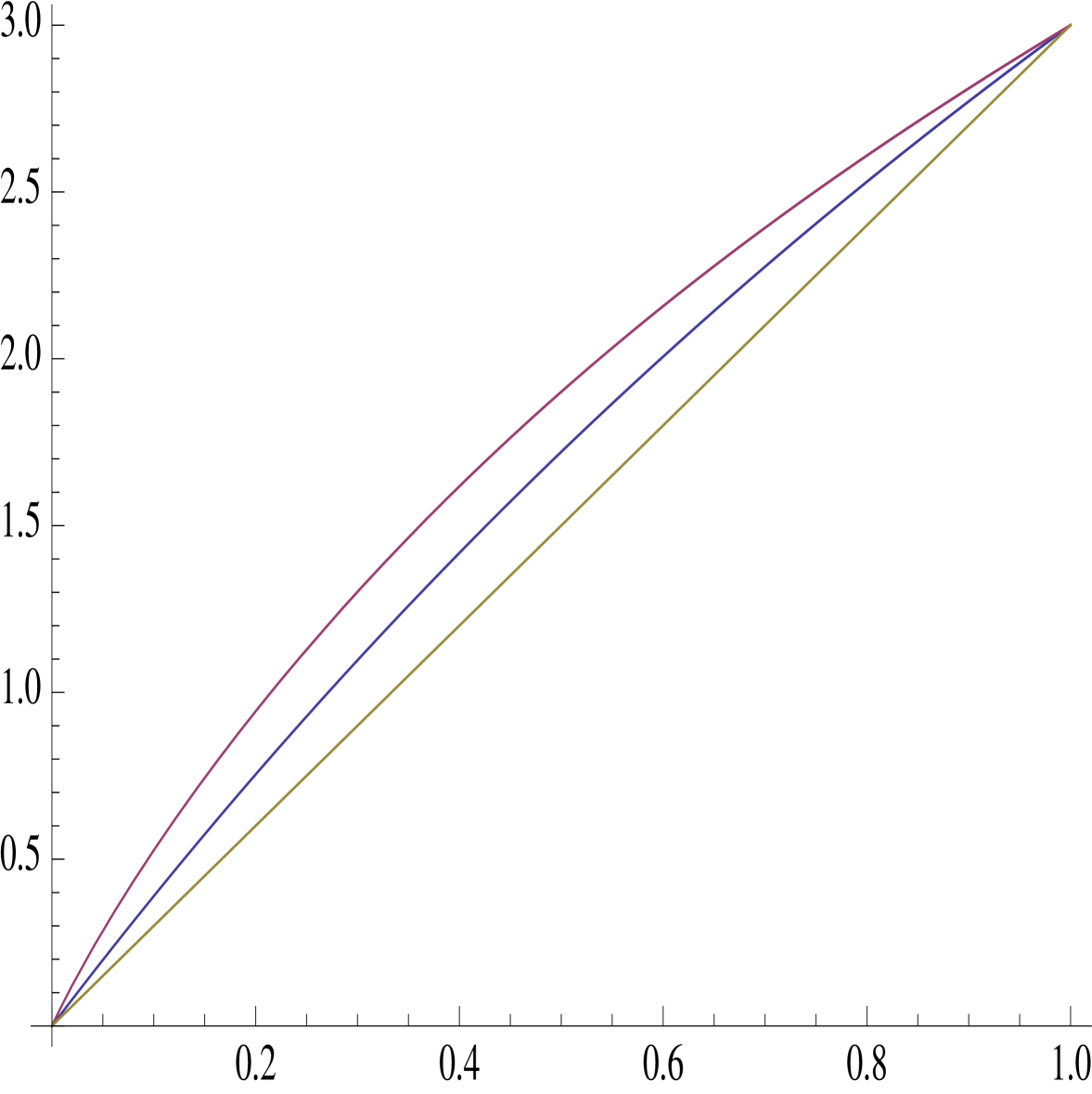
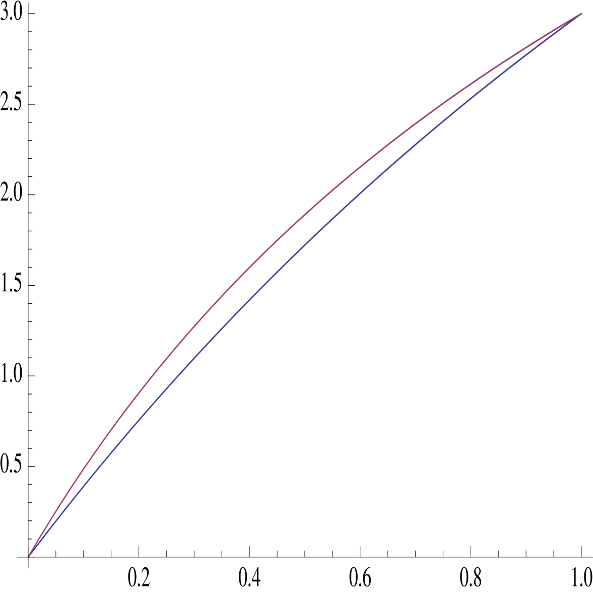
The first example we want to study is the case in which both the temporary and the permanent impact are linear as in Examples 3.3 and 3.7. The motivation is to compare our results with those obtained by Almgren and Chriss (2000). In this example we have set $T=1$ and $K=3$ . The solutions have been numerically calculated using Theorems 3.2 and 3.6 and then plotted in Figures 1 and 2.

It may be observed that, as one would expect, the solutions are not the same and in fact—under the present conditions—our strategy dominates Almgren and Chriss.

4.2. Example

The next example we want to study is the case in which the permanent impact is some power less than 1. Namely $h(x)=x^{3/5}$ , and the permanent is linear. First from Theorem 3.2 we have that

\displaystyle F(f_{1}(u),f^{\prime}_{1}(u)):=sf^{\prime}_{1}(u)\exp\left\{f_{1}(u)+(f^{\prime}_{1}(u))^{3/5}\right\}

and $f_{1}$ is the solution to:

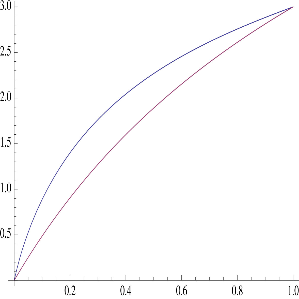
\displaystyle f^{\prime}_{1}-\left(f^{\prime}_{1}+\frac{3}{3}\frac{f^{\prime\prime}_{1}}{(f^{\prime}_{1})^{2/5}}\right)-\left(\frac{3}{5}\right)^{2}\frac{f^{\prime\prime}_{1}}{(f^{\prime}_{1})^{2/5}}-\frac{3}{5}(f^{\prime}_{1})^{3/5}\left(f^{\prime}_{1}+\frac{3}{5}\frac{f^{\prime\prime}_{1}}{(f^{\prime}_{1})^{2/5}}\right)=0,

$f_{1}(0)=0$ and $f_{1}(T)=K$ . In particular, with $T=1$ and $K=3$ as in the previous example we have plotted our result in Figure 3. Note that the sublinear impact has increased the speed of execution. Next, we computed the Markowitz-optimal open-loop trajectory, with $\lambda=1$ by first computing $f_{2}$ as described in Theorem 3.6.

Remark 4.1.

The previous exercise suggests that if one chooses the temporary impact to be sub-linear, the solution—with all the other parameters fixed—will always dominate its linear counterpart. On the other hand, if the temporary impact is super-linear, the solution will be dominated by its linear counterpart.

A natural question is: What is the correct form of $h$ given our model?

5. Remarks on Markovian controls

As pointed out in the introduction, we have only dealt with differentiable deterministic controls—also known as open loop controls. Furthermore, our criteria of optimal is in the Markowitz sense. A couple of natural and reasonable question arise: how can we study feedback controls? How can we optimize with respect to general utility functions? Namely, given some utility function $U$ we want to find a trajectory $c$ such that

\displaystyle\sup_{c\in\mathcal{U}}\mathbb{E}_{t,x}[U(Y)]

where $\mathcal{U}$ is the set of admissible controls and $Y=\xi-KT$ is the execution shortfall. But $\xi$ is in general a very difficult creature to characterize, unless you observe that you may construct a diffusion with the following dynamics:

\displaystyle dX_{t}=\left(c_{t}+\left[g(c_{t})+\frac{dh}{dt}(c_{t})\right]X_{t}\right)dt+\sigma X_{t}dB_{t},\qquad X_{0}=0

that is equal in distribution to $\xi$ , i.e.

\displaystyle\xi_{t}\stackrel{{\scriptstyle\mathcal{D}}}{{=}}X_{t},\qquad\forall t.

Thus

\displaystyle\sup_{c\in\mathcal{U}}\mathbb{E}_{t,x}[U(Y)]=\sup_{c\in\mathcal{U}}\mathbb{E}_{t,x}[U(X_{T}-KT)]

and now you may proceed to derive the Hamilton-Jacobi-Bellman equation. It is precisely this question, which the authors are investigating presently.

References

[1] A. Alfonsi, A. Schied and A. Schulz (2007a) Optimal execution strategies in limit order books with general shape functions, Preprint, QP Lab and TU Berlin.
[2] A. Alfonsi, A. Schied and A. Schulz (2007b) Constrained portfolio liquidation in a limit order book model Preprint, QP Lab and TU Berlin.
[3] R. Almgren and N. Chriss (1999) Value under liquidation, Risk.
[4] R. Almgren and N. Chriss (2000) Optimal Execution of Portfolio Transactions, J. Risk. 3 (2).
[5] R. Almgren, C. Thum , E. Hauptmann, and H. Li (2005) Direct Estimation of Equity Market Impact
[6] D. Bertsimas and D. Lo (1998) Optimal control of execution costs, Journal of Financial Markets. 1.
[7] M.J. Brennan, and E. Schwartz (1979) A Continuous Time Approach to the Pricing of Bonds, J. of Banking and Finance. 3.
[8] P.A. Forsyth (2009) Hamilton Jacobi Bellman Approach to Optimal Trade Schedule, Preprint.
[9] I.M. Gelfand, and S.V. Fomin (2000) Calculus of Variations New York: Dover Publications.
[10] K. Kawaguchi, and H. Morimoto (2007) Long-run average welfare in a pollution accumulation model, J. of Economic Dynamics and Control, 31.
[11] V. Linetsky (2004) Spectral Expansions for Asian (Average Price) Options, Operations Research, 52, pp.856–867.
[12] A. Obizhaeva, and J. Wang (2005) Optimal Trading Strategy and Supply/Demand Dynamics. J. Financial Markets
[13] A. Schied, and T. Schöneborn (2007) Optimal portfolio liquidation for CARA investors, Preprint, QP Lab and TU Berlin

Refer to caption — Figure 1. The graph is plotted with Mathematica. For $\lambda=0$ the blue line (upper line) represents our optimal trading trajectory, the red line is Almgren and Chriss.

Optimal execution of equity with geometric price process

Abstract.

2000 Mathematics Subject Classification:

1. Introduction

2. Auxiliary Results

2.1. The model.

Remark 2.1.

2.2. Averaged geometric and Brennan-Schwartz processes

Proposition 2.2.

Proof.

Remark 2.3.

2.3. Moments of ξ\xi

Corollary 2.4.

Proof.

3. Markowitz Optimal open-loop Trading trajectory

3.1. Execution shortfall

Proposition 3.1.

Proof.

Theorem 3.2.

Proof.

Example 3.3.

Remark 3.4.

Remark 3.5.

Theorem 3.6.

Proof.

Example 3.7.

4. Examples

4.1. Example

4.2. Example

Remark 4.1.

5. Remarks on Markovian controls

References

2.3. Moments of $\xi$