Optimal investment with transient price impact
Abstract
We introduce a price impact model which accounts for finite market depth, tightness and resilience. Its coupled bid- and ask-price dynamics induce convex liquidity costs. We provide existence of an optimal solution to the classical problem of maximizing expected utility from terminal liquidation wealth at a finite planning horizon. In the specific case when market uncertainty is generated by an arithmetic Brownian motion with drift and the investor exhibits constant absolute risk aversion, we show that the resulting singular optimal stochastic control problem readily reduces to a deterministic optimal tracking problem of the optimal frictionless constant Merton portfolio in the presence of convex costs. Rather than studying the associated Hamilton-Jacobi-Bellmann PDE, we exploit convex analytic and calculus of variations techniques allowing us to construct the solution explicitly and to describe the free boundaries of the action- and non-action regions in the underlying state space. As expected, it is optimal to trade towards the frictionless Merton position, taking into account the initial bid-ask spread as well as the optimal liquidation of the accrued position when approaching terminal time. It turns out that this leads to a surprisingly rich phenomenology of possible trajectories for the optimal share holdings.
- Mathematical Subject Classification (2010):
-
91G10, 91G80, 91B06,
49K21, 35R35 - JEL Classification:
-
G11, C61
- Keywords:
-
Utility maximization, transient price impact, singular control, convex analysis, calculus of variations, free boundary problem
1 Introduction
The classical Merton problem [23], [22] of maximizing expected utility from terminal wealth by dynamically trading a risky asset in a financial market has by now been intensively studied and well understood in models with market frictions like transaction costs. We refer to the recent survey by Muhle-Karbe et al. [25] for an overview. In contrast, less is known about utility maximization problems in illiquid market models where the friction is induced by price impact: The investor trades at bid- and ask-prices which are adversely affected by the volume or speed of her current and past trades. Within these models, the vast majority of the existing literature is primarily concerned with the problem of optimally executing exogenously given orders; cf., e.g., the surveys by Gökay et al. [14] and Gatheral and Schied [13]. However, regarding more complex optimization problems such as optimal portfolio choice, explicit characterizations of optimal strategies seem to have been elusive so far. This is notably the case for optimal investment problems on a finite time horizon in the presence of a bid-ask spread and price impact that, rather than being purely temporary or fully permanent, is transient in the sense that the impact of the investors current and past trades on execution prices does not vanish instantaneously but persists and decays over time at some finite resilience rate.
Most of the currently available work on optimal portfolio choice problems in illiquid financial markets focuses on models with purely temporary price impact, i.e., infinite resilience, zero bid-ask spread, and restricts to long-term investors as, e.g., in Guasoni and Weber [18], [16], [17] with constant relative risk aversion, in Forde et al. [10] with constant absolut risk aversion or in Gârleanu and Pedersen [11], [12] with mean-variance preferences. In the latter papers, the authors also take into account finite resilience. For investors having a finite planning horizon but still solely facing temporary price impact, asymptotic results have been obtained by Moreau et al. [24] and in a more general setup in Cayé et al. [5]; cf. also Chandra and Papanicolaou [7] for a pertubation analysis. The results from [24] are also used as a building block to describe asymptotically optimal trading strategies under highly resilient price impact in Kallsen and Muhle-Karbe [20], or in Ekren and Muhle-Karbe [9] in the setting of [11]. In all the above cited papers, trading strategies are confined to be absolutely continuous.
In the present paper, we propose a price impact model which goes beyond the block-shaped limit order book model of Obizhaeva and Wang [26] by allowing for both selling and buying stock. Specifically, our model determines bid- and ask-prices via a coupled system of controlled diffusions, giving us the possibility to specify market depth, tightness and resilience: the three dimensions of liquidity identified in the seminal work by Kyle [21]. The coupled bid- and ask-price dynamics induce convex liquidity costs on the trading strategies which are allowed to be singular and comprise non-infinitesimal block trades as in [26]. In fact, our model is closely related to the one proposed in Roch and Soner [28] which is an extension of the illiquid market model approach introduced by Çetin et al. [6] in the sense that it additionally takes into account finite resilience and a bid-ask spread. In contrast, our model captures recovery of the bid- and ask-prices by a reversion to each other rather than towards some auxiliary reference price process. Moreover, our illiquidity parameters, i.e., market depth and resilience, are constant in order to preserve tractability.
We provide existence of an optimal solution to the corresponding classical problem of maximizing expected utility from terminal liquidation wealth at some finite planning horizon. In its simplest version, our price impact model is an illiquid variant of a Bachelier model with convex liquidity costs which are levied on the agent’s trading activity. For an investor who exhibits constant absolute risk aversion, it turns out that the resulting singular optimal stochastic control problem readily reduces to a deterministic optimal tracking problem of the optimal frictionless buy-and-hold Merton portfolio in the presence of convex costs. Instead of the more common dynamic programming methods which lead to the challenge of solving a three-dimensional free boundary problem induced by a Hamilton-Jacobi-Bellman partial differential equation, we exploit a convex analytic approach. Deriving first order conditions in terms of the (infinite dimensional) subgradients of the convex cost functional allows us to construct explicitly the solution to the singular control problem by calculus of variations. As a consequence, we are able to describe analytically the free boundaries of the buying-, selling and a no-trading region in the underlying three-dimensional state space for the optimally controlled dynamics of the spread and the risky asset holdings with respect to the remaining time to maturity.
Our explicit results make transparent how the optimal strategy has to comprise several aspects. As already expected by the work in Guasoni and Weber [18], [16], [17], Forde et al. [10], and Gârleanu and Pedersen [11], [12], it is indeed optimal to trade towards the optimal frictionless portfolio while taking into account the initial bid-ask spread as well as the available time horizon. Specifically, since liquidation is costly in the present setup, the optimizer also has to take care of optimally unwinding his accrued position when approaching terminal time. It turns out that already in this elementary illiquid Bachelier model the interaction of market tightness, finite resilience, desired position targeting and optimal liquidation at a finite time horizon permits a surprisingly rich phenomenology of possible trajectories for the optimal share holdings. In this regard, our optimization problem is substantially different from the infinite horizon and zero spread frameworks considered in the papers cited above. Our findings also complement and extend the explicit results on the optimal order execution problem as studied in Obizhaeva and Wang [26] in a similar Bachelier-type setting.
The paper most closely related to ours is Soner and Vukelja [30]. Therein, the authors adopt the model from Roch and Soner [28] without bid-ask spread in a Black-Scholes framework with constant resilience and stochastic market depth proportional to the risky asset price. Using the dynamic programming principle and the notion of viscosity solutions, the problem of maximizing expected utility from terminal liquidation wealth for CRRA investors with finite planning horizon is studied. Compared to our results, their more general framework comes at the cost that a characterization of the optimal strategy is only possible numerically via a discrete-time approximation scheme.
The rest of the paper is organized as follows. In Section 2 we introduce a price impact model. Section 3 outlines the problem of maximizing expected utility from terminal liquidation wealth in our model and provides existence of an optimal solution in a general setup. In the specific case when market uncertainty is generated by an arithmetic Brownian motion with drift and the investor exhibits constant absolute risk aversion, we show that the optimal singular stochastic control problem has a deterministic solution which we construct explicitly. This is presented in Section 4. Technical proofs are deferred to Section 5.
2 A price impact model
We fix a filtered probability space satisfying the usual conditions of right continuity and completeness and consider an investor whose trades in a risky asset affect its market prices in an adverse manner. For our specification of her price impact, we propose a variant of the block-shaped limit order book model introduced by Obizhaeva and Wang [26]. Specifically, the investor’s trading strategy is described by a pair of predictable, nondecreasing, right-continuous processes where , denote , respectively, the cumulative purchases and sales of the risky asset until time . We set . Trading takes place via market orders in an idealized block-shaped limit order book at the best bid- and ask-prices and . Their dynamics are specified as the solution to the following coupled system of controlled diffusions
| (1) |
with given parameters , , and . The interpretation of the bid- and ask-price dynamics in (1) is the following: Both processes and are driven by some common exogenous fundamental random shock modeled by a continuous semimartingale with initial value . The process can also be regarded as the unaffected price process. Due to finite market depth which can be interpreted as the height of a block-shaped limit order book, a buy order incurs an impact and increases the best ask-price by the amount whereas the best bid-price is not directly affected. After completion of each buy trade, ask- and bid-prices revert to each other at some resilience rate . The effects of sell orders on the best bid-price in (1) are analogous. Note that price impact is transient and does not vanish instantaneously but persists and decays over time at a finite exponential rate . We will assume for simplicity that both illiquidity parameters, i.e., the instantaneous price impact factor as well as the resilience rate , are constant. According to the bid- and ask-price dynamics in (1), the controlled evolution of the bid-ask spread is described by
| (2) |
with initial value and right-continuous solution
| (3) |
Let us now derive the investor’s wealth dynamics corresponding to a trading strategy . First, we associate to the self-financing portfolio process with some given initial values where denotes the amount of cash and the number of shares of the risky asset held at time . Assuming zero interest rates, the self-financing condition dictates that the cash balance changes only due to trading activity , i.e., we postulate that
with , respectively. Observe that the effective execution price to, e.g., buy a not necessarily infinitesimal quantity of shares at time is given by where accounts for the impact a non-infinitesimal order incurs; cf., e.g., also Alfonsi et al. [1] or Predoiu et al. [27]. Analogous considerations apply for sell orders. The investor’s total wealth at any time is now expressed in terms of the liquidation value of her current portfolio. That is, we define the investor’s liquidation wealth process associated to her portfolio process with trading strategy and initial endowment as
| (4) |
We set the initial value to . Note that the liquidation value in (4) decomposes into two parts: The first part represents the portfolio’s book value , where the value of the position in the risky asset is measured in terms of the mid-quote price . The second part accounts for the corresponding liquidation costs which are incurred by the bid-ask spread as well as the instantaneous price impact when unwinding in one single block trade the shares. Following lemma shows that the dynamics of the liquidation wealth process in (4) conveniently separate into the common frictionless wealth and a nonnegative, convex cost functional.
Lemma 2.1.
The liquidation wealth process of a strategy defined in (4) allows for the decomposition
| (5) |
where denotes the liquidity costs defined as
| (6) | ||||
with initial value . In particular, for all the functional is convex in and satisfies
| (7) |
Observe that the quantity in (5) represents by definition the initial wealth’s book value or initial frictionless wealth of strategy with initial endowment .
Remark 2.2.
-
1.
Compared to other price impact models which are used in the literature in the context of optimal portfolio choice, our price impact in (1) depends on the trading volume of the investor in the spirit of Obizhaeva and Wang [26] and not on the trading rate as, e.g., in Gârleanu and Pedersen [11], [12] or Forde et al. [10]. These papers adopt purely temporary price impact as proposed by Almgren and Chriss [2]. In Guasoni and Weber [18], [16], [17] temporary price impact is not only induced by the trading rate but also depends on the investor’s total wealth. Our model captures transient price impact which decays only gradually over time. As a consequence, trading strategies are no longer restricted to be absolutely continuous but also comprise non-infinitesimal block trades. In fact, our modeling approach is similar to the one proposed in Roch and Soner [28] where the authors allow for more general stochastic dynamics for the market depth and the resilience rate. Another difference is that our bid- and ask-prices in (1) revert to each other and not to some reference price as in [28].
-
2.
Recall that proportional transaction costs as considered, e.g., in Davis and Norman [8], are linear in the risky asset holdings. Temporary price impact which is linear in the trading rate of absolutely continuous strategies as considered in Gârleanu and Pedersen [11], [12] or Guasoni and Weber [18], [17] induces quadratic liquidity costs on the latter. The authors in Forde et al. [10], Guasoni and Weber [16] and Cayé et al. [5] allow for nonlinear price impact which introduces a dependence of the incurred trading costs on a fractional power of the turnover rates. In our model above, price impact in (1) is still linear in the trading strategy but the induced liquidity costs in (6) are convex in rather than purely quadratic because of the emergence of the absolute value function.
3 Optimal investment problem
We consider an investor who aims to trade optimally in the price impact model introduced in Section 2. The investor’s preferences are described by a utility function in which is strictly concave, increasing and bounded from above. She wants to maximize expected utility from her terminal liquidation wealth at some finite planning horizon as defined in (4) by following a trading strategy with given initial endowment in cash and shares of the risky asset. Her corresponding initial wealth and the associated liquidation costs are denoted by and for some given initial bid-ask spread . In other words, in view of Lemma 2.1, the agent’s aim is to solve the optimization problem
| (8) |
over all admissible trading policies
The main tool which allows us to provide existence of an optimal strategy to the maximization problem in (8) is given by the following convex compactness result for processes of finite variation.
Lemma 3.1 (Guasoni [15], Lemma 3.4).
Consider a sequence of strategies such that is bounded in . Then there exists a strategy and a sequence of cofinal convex combinations, i.e., for all , converging to weakly on :
| (9) |
Another important ingredient is provided by the continuity of the liquidation wealth in given in (5).
Lemma 3.2.
Let and let be a sequence of strategies with the same initial endowment such that weakly on on all of . Then it holds that
As a consequence, due to convexity of the liquidity cost functional in by virtue of Lemma 2.1, we obtain the following existence and uniqueness result for the optimization problem in (8).
Theorem 3.3.
There exists a unique strategy such that for all strategies .
Proof.
Consider a maximizing sequence such that
We can assume without loss of generality that the sequence belongs to the level-set . Moreover, due to Lemma 5.1 below, it holds that is -bounded. Hence, by virtue of the compactness result in Lemma 3.1, there exists a strategy and a sequence of convex combinations such that a.s. weakly on for . We claim that is the optimal solution to problem (8). Indeed, since the liquidity costs are convex, is again a maximizing sequence. Specifically, given a finite number of strictly positive weights of , we have
where we also used monotonicity and concavity of . Taking expectations and passing to the limit in the above inequality yields . Moreover, by continuity of the liquidation wealth provided in Lemma 3.2 and Fatou’s Lemma we obtain
Uniqueness of the optimizer follows from strict concavity of the utility function and again convexity of the liquidity costs. ∎
4 Illiquid Bachelier model with exponential utility
Let us investigate the utility maximization problem from terminal liquidation wealth as formulated in (8) in the specific case when market uncertainty in our price impact model (1) is generated by a Brownian motion with drift and volatility . That is, we assume that the unaffected price process is given by
| (10) |
where denotes a standard Brownian motion on the given filtered probability space . In addition, we assume that the inverstor’s preferences are prescribed by an exponential utility function
with constant absolute risk aversion parameter . In this setup, the optimization problem in (8) becomes
| (11) |
Note that for exponential utility, the optimal strategy in (11) does not depend on the investor’s initial frictionless wealth . By virtue of Theorem 3.3, there exists a unique optimal solution to the maximization problem in (11) for any time horizon , initial position in the risky asset and any initial bid-ask spread
Remark 4.1 (Frictionless case).
It is well known in the literature that in the frictionless case with , i.e., in (1) and in (6) for any , the optimal strategy to problem (11) (with initial position ) is simply a deterministic buy-and-hold-strategy given by
Here, and denote the Dirac measure in and , respectively. Put differently, the optimal frictionless share holdings in the risky asset are constant and given by the so-called Merton portfolio
| (12) |
which is acquired at time and unwound at time with, respectively, an initial and a final block trade.
When taking into account illiquidity frictions as in our setup, that is, price impact induced by finite market depth as well as market tightness imposed by the bid-ask spread, it is intuitively sensible to expect the following: Instead of directly implementing the desired frictionless Merton position in (12), the optimal frictional portfolio for problem (11) will gradually trade towards the latter. In fact, in the presence of price impact , it turns out that problem (11) readily translates into a deterministic optimal tracking problem of the frictionless optimal portfolio position .
Proposition 4.2.
For given time horizon , initial position and initial spread , the optimal investment strategy of the maximization problem in (11) is deterministic and coincides with the minimizer of the convex cost functional
| (13) |
with .
Proof.
We give an argument similar to Schied et al. [29], but extend it to also cover unbounded strategies. For notational convenience, let us define the cost functional
for all and let us set . Next, let be such that . We will argue below that for such the density
| (14) | ||||
induces a probability measure on . Then we can write
| (15) | ||||
with equality holding true for the unique deterministic minimizer of . Thus, the maximizer of the right-hand side in (15) over all admissible strategies which corresponds to our original problem in (11) is actually given by the deterministic strategy attaining the value .
It remains to verify that (14) indeed defines a probability measure for with , i.e., such that
| (16) |
This will be accomplished by verifying Kazamaki’s criterion for the process . To this end, observe first that we can assume without loss of generality that and so, with and , we can use (7) to estimate
for . With (16) and the fact that it thus follows that which guarantees uniform integrability of . Moreover, we have
which is finite because of (16) and (7). It follows that indeed satisfies Kazamaki’s criterion. ∎
Remark 4.3.
-
1.
For deterministic strategies the liquidation wealth in (5) in the present illiquid Bachelier model is normally distributed. Hence, the maximization problem in (11) and thus the minimization problem in (13) is equivalent to the problem of maximizing a mean-variance criterion given by
cf. also the discussion in Schied et al. [29].
-
2.
The minimization problem in (13) can be regarded as a deterministic optimal tracking problem of the frictionless Merton portfolio in the presence of trading costs measured by . That is, the optimal strategy seeks to minimize both the squared deviation of its share holdings from the preferred constant position of (12) as well as the incurred liquidity costs which are levied on its trading activity due to market tightness and finite market depth. In addition, liquidation is costly in the current setup. Therefore, besides trading towards , the optimizer also has to take into account unwinding the accrued position in the risky asset in an optimal manner when approaching terminal time .
-
3.
The deterministic optimal tracking problem in (13) is similiar to the stochastic tracking problem studied in Bank et al. [4] (cf. also Bank and Voß [3] for a more general framework). Therein, the authors investigate the problem of minimizing the -distance of a portfolio process from a given predictable stochastic target process in the presence of temporary price impact as in Almgren and Chriss [2]. This means that investment strategies are restricted to be absolutely continuous and quadratic costs are levied on the respective trading rates . The process represents, e.g., an optimal investment or hedging strategy adopted from a frictionless setting. In the current setup in (13), liquidity costs are induced by market tightness and transient price impact à la Obizhaeva and Wang [26] and strategies are allowed to be singular.
4.1 First order optimality conditions
Since the objective functional of the minimization problem in Proposition 4.2 is convex, tools from convex analysis and calculus of variations can be employed to derive a characterization of the optimal solution in terms of sufficient first order conditions. Specifically, let us note that the convex functional is supported on by the infinite-dimensional buy- and sell-subgradients defined as
| (17) | ||||
| and | ||||
| (18) | ||||
in the sense of Lemma 4.5 below.
Remark 4.4.
The map appearing in the definition of the buy- and sell-subgradients in (17) and (18) represents the subgradient of the absolute value function (cf. proof of Lemma 4.5 in Section 5) and therefore allows for an arbitrary value when . In this case the subgradients are actually set-valued. The dependence on the value is indicated by the left-hand superscript in the operator symbols and . To alleviate notation, we will simply write , and most of the time unless a specification of the value becomes necessary.
Lemma 4.5.
For any nondecreasing, right-continuous process with , let us further define the set
| (19) |
and observe that for any continuous we have
Having at hand the subgradients in (17) and (18), we can now formulate sufficient first order optimality conditions for the minimization problem stated in Proposition 4.2.
Proposition 4.6 (First order conditions).
The strategy in solves the optimization problem in (13) if the following conditions hold true:
-
(i)
for all with ‘=’ on the set ,
-
(ii)
for all with ‘=’ on the set .
In case , the conditions in (i) and (ii) are meant to hold for and with some .
Proof.
Assume that satisfies conditions (i) and (ii) (for some suitable in case ) and let be an arbitrary competing strategy with the same initial endowment . Then, by virtue of Lemma 4.5 above, it holds that
By our assumptions (i) and (ii) the right-hand side is nonnegative which implies . ∎
Remark 4.7.
In view of Lemma 4.5, the quantities and in (17) and (18) can be regarded as (lower bounds for) the marginal costs which are incurred by an additional infinitesimal buy order and sell order at time , respectively, otherwise following strategy . Hence, an optimal strategy which satisfies the first order conditions in Proposition 4.6 acts so as to keep these additional marginal costs from intervention always nonnegative and only intervenes, i.e., buys or sells the risky asset, when the corresponding marginal costs or vanish. In this regard, observe that, loosely speaking, the subgradients in (17) and (18) at time can be interpreted as assessing for the future period the trade-off between deviating from the target , the incurred spread as well as the magnitude of the final position .
Due to market tightness, it is intuitively sensible to expect that an optimal strategy satisfying the first order conditions in Proposition 4.6 will never purchase and sell the risky asset at the same time. In fact, this holds true in our setting and is a direct consequence of the structure of the subgradients.
Lemma 4.8.
For any strategy , , we have
Remark 4.9 (Dynamic programming principle).
Note that for any strategy the subgradients of our functional in (17) and (18) at time only depend on the values , , , , the remaining time to maturity and the future evolution of the strategy . This property together with the uniqueness of the optimal solution to problem (13) implies that the dynamic programming principle (or so-called Bellman optimality) holds true in our setting. Specifically, let denote the unique optimal strategy for problem (13) with time horizon , initial position and initial spread which satisfies the first order conditions in Proposition 4.6. From now on, we will use the notation to emphasize the dependence of the optimal control on the problem data . Then for any we have that the strategy
is optimal for problem (13) with problem data , i.e., time horizon , initial spread and initial position . Indeed, observe that
holds true which implies that satisfies the first order conditions in Proposition 4.6 and is thus optimal.
4.2 The state space
We want to solve the optimization problem formulated in (13) for any given problem data , i.e., for any time horizon , initial spread and initial position in the risky asset. For this purpose, let us introduce the three-dimensional state space
| (20) |
with time to maturity , spread and number of shares . For any triplet or problem data in the state space we want to identify the corresponding unique optimal strategy with and which minimizes the functional in (13) for time horizon (cf. Remark 4.11 below for our convention in the special case ). More precisely, we want to describe the evolution of the optimally controlled system in the state space . Intuitively, the first order optimality conditions formulated in Proposition 4.6 suggest a separation of the state space into two action regions – a buying- and a selling-region – as well as a non-action or waiting-region for the optimizer . Loosely speaking, depending on whether the optimally controlled triplet at time is located in the buying-, selling- or waiting-region, the corresponding optimal strategy buys, sells or does not do anything, respectively, at this time instant . In fact, Proposition 4.6, Lemma 4.8 as well as Remark 4.9 motivate the following definition of the buying-, selling- and waiting-region.
Definition 4.10 (Buying-, selling-, waiting-region).
-
1.
We define the buying-region as
(21) and the boundary of the buying-region as
(22) -
2.
We define the selling-region as
(23) and the boundary of the selling-region as
(24) -
3.
We define the waiting-region as
(25) where , respectively.
Remark 4.11.
- 1.
-
2.
By definition in (20) problem data or triplets with also belong to the state space . Hence, we have to find a convention for how to specify the associated optimal strategies with and . In view of the subgradients in (17) and (18) we have
Thus, in case it holds that and . Therefore, we stipulate that the associated optimal strategy is given by and , i.e., it unwinds with a single block sell order the position . Analogously, in case we have and and thus we set as well as , i.e., the optimal strategy clears out its short position by executing a single block buy order. In case , we have
for all . We make the convention that the associated optimal strategy is simply defined as .
-
3.
Note that our convention in 2.) together with the dynamic programming principle from Remark 4.9 entails that any optimal strategy with a final position in the risky asset in fact unwinds its remaining shares with a single block order.
4.3 Main result
Our main result is an explicit description of the buying- and selling-region and in the state space defined in Definition 4.10. Specifically, it turns out that the free boundaries and can be described analytically as the graph of two free boundary functions and defined on the time-to-maturity and spread domain . All the results in this section will be proved in Section 5.
Theorem 4.12.
In fact, the behaviour of optimal strategies with initial problem data in , , or can be readily deduced from the definition of the buying-, selling- and waiting-region in (21), (23) and (25), together with the dynamic programming principle from Remark 4.9.
Remark 4.13.
-
1.
For each problem data , i.e., in view of (27) in Theorem 4.12, it follows from the definition of and in (23) and (24) that the optimal strategy will actually “jump” with an initial impulse block sell order of size satisfying the equation
(33) to the triplet which belongs to by virtue of (28). Thereafter, it coincides with the corresponding optimal strategy which does satisfy in line with the definition of in (24); cf. proof of Theorem 4.12 below. Similarly, for each problem data , i.e., in view of (29) in Theorem 4.12, the optimal strategy will “jump” with an initial impulse block buy order of size satisfying the equation
(34) to the triplet in by virtue of (30) and then will coincide with the corresponding optimal strategy . Again it will hold that in line with the definition of in (22).
-
2.
For any problem data , i.e., in view of (31) in Theorem 4.12, the optimal strategy will remain inactive until the first time that either
(35) or
(36) holds true. That is, the triplet belongs to or due to (28) and (30), respectively. On the remaining time interval the optimal strategy then coincides with the corresponding optimal strategy . Note that will hold true due to the definition of the boundaries in (24) and (22), respectively. For the case where neither (35) nor (36) allows for a solution , it will be optimal to remain inactive all along . Recall from our convention in Remark 4.11, 2.) that any non-zero final position in the risky asset will be unwound with a single block trade.
As a consequence of Remark 4.13, it suffices to characterize all optimal strategies with initial problem data which belong to the boundaries or . The next two corollaries summarize how these strategies can be computed explicitly.
Corollary 4.14 (Selling boundary).
Let . Then we have . The optimal share holdings and spread dynamics satisfy
| (37) |
In particular, solves the second order ODE
| (38) |
on with initial conditions
| (39) |
where and are given as in (82).
Remark 4.15.
For the buying boundary, the description of optimal strategies becomes a bit more involved as one has to distinguish three cases depending on the size of the initial spread:
Corollary 4.16 (Buying boundary).
Let and let , , be given as in (69), (72), (78), respectively, as well as , as defined in Lemmas 5.6 and 5.7.
-
1.
If , then we have . The optimal share holdings and spread dynamics satisfy
(40) In other words, solves the second order ODE
(41) on with initial conditions
(42) -
2.
If , then we have with . The optimal share hodings and spread dynamics satisfy
(43) In this case, the ODE dynamics in (41) are satisfied by on with terminal conditions
(44) -
3.
If , then on .
Moreover, in both cases 2.) and 3.), if
| (45) |
then it holds that
| (46) |
Remark 4.17.
Notice that except for a possible initial and final singular block trade (recall Remarks 4.11, 2.) and 4.13), share holdings of optimal strategies turn out to be absolutely continuous. This is in line with the optimal execution strategies computed in Obizhaeva and Wang [26]. During these periods of steadily buying or selling, the dynamics of the optimal share holdings are prescribed by the same second order ODE in (38) and (41). In fact, satisfying the ODE with the corresponding boundary conditions forces, respectively, the buy-subgradient or sell-subgradient to vanish which is in line with the first order optimality conditions in Proposition 4.6. Also note that while the optimal strategy is continuously buying- or selling, the optimally controlled triplet evolves along the boundary of the buying- or selling-region in the state space ; cf. (37), (40), and (43) together with Theorem 4.12.
4.4 Illustration
Let us illustrate with a numerical example the separation of the three-dimensional state space into a buying-, waiting- and selling-region as characterized in Theorem 4.12 along with trajectories of optimal strategies as described in Corollaries 4.14 and 4.16 together with Remark 4.13. All explicit representations of the free boundaries and as well as of the illustrated optimal strategies can be found in Section 5.3. As for the model parameters, we simply choose
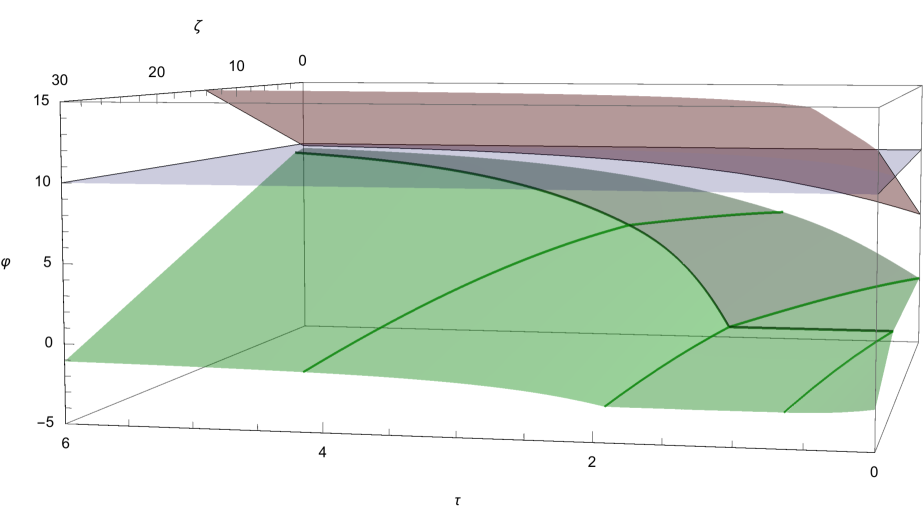
Figure 1 shows the three-dimensional state space with time to maturity , spread and number of shares . The blue plane represents the constant optimal frictionless Merton position at level , henceforth referred to as Merton plane. The upper red surface is the free boundary of the selling region as characterized in Theorem 4.12, i.e.,
with defined in (66). The lower green surface depicts the free boundary of the buying region , that is,
with defined in (90) – (94). Observe that actually decomposes into seven parts (cf. Section 5.3.1 for more details). As expected by the formulation of the optimization problem in Proposition 4.2 as an optimal trading problem towards the constant Merton portfolio, one can observe in Figure 1 that the green boundary of the buying region is always below the Merton plane. Moreover, at least for large maturities and large initial spread values , the red boundary of the selling region is above the Merton position. However, notice that it falls below the latter for small maturities and small spread values . That is, even though the position in the risky asset is below the target portfolio , the short time horizon forces the optimizer to start liquidating the share holdings right away. Recall from Remark 4.3 2.) that this results from the fact that liquidation is costly. Hence, the optimal control also has to take into account unwinding the accrued position when terminal time comes close. The same interpretation also applies for the “plateau” of the buying boundary at level for small maturities and small spread values. In other words, starting with a short position in the risky asset and facing a short time horizon, it is optimal to simply clear out the short position even before the time horizon is reached. Mathematically, the presence of this plateau is due to the dependence of the subgradients in (17) and (18) on in case where the optimal terminal position is equal to zero (again cf. Section 5.3.1 for the details).
Figure 2 depicts the evolutions of some optimal share holdings for different problem data as functions in time to maturity with . The corresponding spread dynamics are presented in Figure 3. The trajectories of the associated optimally controlled state processes embedded in the three-dimensional state space are illustrated in Figure 4.
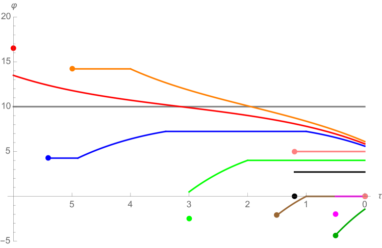
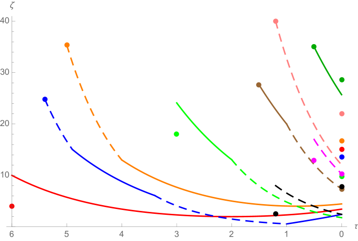
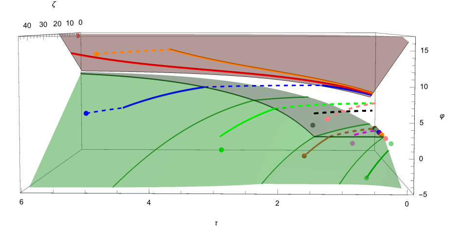
The red policy is similar to the optimal liquidation strategies computed in Obizhaeva and Wang [26] for a risk-averse investor, though with a non-zero but small initial spread (recall Remark 4.15). Observe that the trajectory starts in the selling region with an initial position in the risky asset above the Merton portfolio. Thus, as described in Remark 4.13 1.), the policy jumps with an initial block sell order to the boundary of the selling region and then continues steadily trading towards the Merton level by selling the risky asset as described in Corollary 4.14. In particular, note that the strategy steadily sells until maturity even after reaching the targeted Merton level . As characterized in (37) (recall also Remark 4.17), the optimally controlled trajectory evolves along the boundary . At the end, following our convention from Remark 4.11 2.), the remaining shares are liquidated with a single block sell order. Similarly to the red policy, the orange policy also has an initial position above Merton but it comes along with a large initial spread. As a consequence, the corresponding problem data belongs to the waiting region . In this case it is optimal to exploit the resilience effect first and to be inactive until the value of the spread is sufficiently small so that it becomes optimal to trade towards . This happens when the trajectory hits the boundary of the selling region as described in Remark 4.13 2.). The blue policy is an optimal strategy which decomposes into a waiting-, buying-, waiting- and selling part. The initial share holdings are below the desired Merton position but similar to the orange policy the initial spread value is too large to intervene immediately. Again the optimal strategy is inactive until the spread is sufficiently small so that it becomes optimal to trade towards and to buy shares according to the description in Corollary 4.16 2.), once the trajectory hits the boundary of the buying region . Note that the optimizer is exploiting the resilience effect also while it is purchasing the risky asset since the value of the spread continues to decrease; see Figure 3. Thereafter, when the position in the risky asset is close enough to Merton with respect to the remaining time, the optimizer becomes inactive again. During this waiting period the spread continues to decay until the trajectory hits the boundary of the selling region as characterized in (46). The optimal control then starts to continuously unwind its accrued position until terminal time. The black policy is of buy-and-hold type with initial and final block trades, remarkably similar to the frictionless optimizer. This is due to the fact that the time horizon is very small together with a small initial spread which makes it optimal to execute a single initial block buy order from to towards the Merton position but without reaching it. Thereafter, the optimizer follows the characterization in Corollary 4.16 3.) where (46) does not occur. The pink policy does not trade at all and unwinds at the end. The brown policy starts with a short position in the risky asset. Again, since time horizon is relatively short, it merely clears out its short position in the risky asset as described in Corollary 4.16 2.) even before the end and then remains at level until the time horizon is reached. Similarly for the magenta policy but instead with a single initial block buy order. The dark green policy continuously liquidates an initial short position until the end and correspond to the case described in Corollary 4.16 1.).
To sum up, the numerical example illustrates how the optimal strategies which maximize expected utility from terminal liquidation wealth in our illiquid Bachelier model exhibit for different time horizons , initial spread values and initial endowments a rich phenomenology of possible trajectories.
5 Proofs
5.1 Proofs for Sections 2 and 3
We start with the computation of the dynamics of the liquidation wealth process defined in (4) and the associated liquidity costs stated in Lemma 2.1.
Proof of Lemma 2.1. To alleviate the notation, let us introduce the mid-quote price process for all with initial value . Applying integration by parts in (4) as in, e.g., Jacod and Shiryaev [19], Definition I.4.45, yields
| (47) | ||||
where we used the fact that by virtue of [19], Theorem I.4.52. Moreover, note that Proposition I.4.49 a) in [19] implies for all , because is predictable and is of finite variation. Inserting this, the spread dynamics (2) as well as the dynamics of the mid-quote in (47) above yields
| (48) |
This motivates to define the liquidation cost functional as
| (49) |
with . Using once more the spread dynamics in (2) we can write . Inserting this expression in (49) gives us
| (50) |
Again, integration by parts as in [19], Definition I.4.45, allows us to write
| (51) | ||||
| (52) |
Plugging back (51) and (52) into (50), using the definition of as well as the fact that for all (cf. Proposition I.4.49 a) in [19]) finally yields
| (53) |
Next, by using the explicit representation of the spread in (3) and introducing the process for all we obtain
| (54) | ||||
Once more due to [19], Proposition I.4.49, observe that we have
| (55) |
In addition, it holds that for all . Thus, using this representation as well as (55) in (54), and plugging the resulting term back into (53) yields the desired form of the liquidity cost functional in (6). Finally, one can easily observe that the functional in (6) is convex in for each . Moreover, using the lower estimate for all , we obtain the lower bound of as claimed in (7). ∎
In order to apply Lemma 3.1 in our setting in the proof of Theorem 3.3, we need the following lemma.
Lemma 5.1.
For the level-set , is -bounded.
Proof.
First, observe that due to convexity of the liquidity cost functional in by virtue of Lemma 2.1 as well as concavity and monotonicity of the utility function , the level-set is a convex set. As a consequence, it holds that . Next, note that for any the liquidation wealth as given in (5) can be bounded from above by
| (56) |
with , where we used integration by parts, the fact that the semimartingale is continuous and the lower bound from Lemma 2.1 for some constant . Henceforth, to alleviate the presentation, let us assume without loss of generality that as well as . Due to the upper bound in (56), we obtain for all the estimate
Hence, together with the fact that is bounded from above, it must hold for the negative part that
Moreover, since is strictly concave and increasing which yields and thus for all , we obtain
| (57) |
Finally, observe that the -boundedness in (57) implies that the set is bounded in . ∎
The last ingredient for the proof of Theorem 3.3 is the continuity of the liquidation wealth in .
Proof of Lemma 3.2. We fix . By weak convergence of to on , we obtain that for and all such that ; cf. the representation of the spread in (3). In particular, it holds that -a.e. on because the number of jumps of , is countable. At the time is uniformly bounded in and since so is . Thus, by dominated convergence, we get for any that Moreover, we obviously have that . Hence, referring to the representation of the liquidity costs in (6), we can conclude that . Next, concerning the stochastic integral of with respect to the continuous semimartingale in the liquidation wealth in (5), we obtain, after applying integration by parts, the expression
where we again used weak convergence of on for all and the continuity of . In summary, we obtain pointwise for all as desired. ∎
5.2 Proofs of Lemma 4.5 and Lemma 4.8
Next, let us compute the infinite-dimensional subgradients in (17) and (18) of the convex cost functional on given in (13).
Proof of Lemma 4.5. Let us define the deviation functional
| (58) |
on . Then the convex cost functional in (13) can be written as . We will proceed in three steps.
Step 1: Let us start with the computation of the subgradients of the liquidity cost functional given in (6). Observe that for any with and any we obtain
| (59) | ||||
Note that we have the lower bound and , where we denote by the subgradient of the function with ; cf. Remark 4.4. Plugging back these lower bounds into (59) and passing to the limit yields
| (60) | ||||
Next, let us express every term in (60) as an integral with respect to either or . Using (3) for the spreads and as well as Fubini’s Theorem, we can rewrite the first term in (60) as
Moreover, using that as well as allows us to finally write (60) as
| (61) | ||||
where we set
Step 2: Let us now compute the subgradients of the deviation functional defined in (58). Again, for any with and any we obtain
and hence, together with Fubini’s Theorem, we arrive at
Consequently, we can write
| (62) |
where we set
| (63) |
5.3 Proofs of Section 4.3
In this section we prove our main Theorem 4.12 together with Corollaries 4.14 and 4.16. We start with introducing the two key objects, that is, the free boundary functions and on the domain .
5.3.1 The free boundary functions
Introducing the function is straightforward. Recall that and . We set
| (64) |
and denote
| (65) |
On the domain , the free boundary function will then be defined as
| (66) |
Let us note the following property which can be easily checked:
Lemma 5.2.
We have for all , , since and for all . ∎
Remark 5.3.
By a slight abuse of the definition of the function in (66) which is only confined to the positive half-plane , we will also use for the notation with the obvious meaning .
In contrast to in (66), introducing the free boundary function on the domain is much more intricate and necessitates several auxiliary constants and functions. First, let denote the unique strictly positive solution to the equation
| (67) |
and let denote the unique solution to the equation
| (68) |
Next, we introduce the mapping for all via
| (69) |
with
| (70) | ||||
| (71) |
and
| (72) |
where
| (73) |
We further set
| (74) |
Let us mention that since satisfies (67) it holds in (70) that
| (75) |
Moreover, direct computations reveal that
| (76) |
as well as
| (77) |
It will turn out that specifies a curve which is embedded in the free boundary in the state space . The next lemma collects some useful properties concerning the maps introduced in (70), (71), (74), respectively, as well as this curve. We also refer to the graphical illustration in Figure 5 below in this context.
Lemma 5.4.
-
1.
We have and . Moreover, on the interval , the map is strictly increasing. In particular, it holds that on .
-
2.
We have and as well as . Moreover, on the interval , the map is strictly increasing and the map is stricly decreasing. In particular, it holds that on .
-
3.
The map , , is continuous, flat on , and strictly decreasing on with . In particular, we have for all .
-
4.
The map , , is continuous, flat on , and strictly increasing on with . In particular, we have for all .
Proof.
Next, let us introduce for all , and the mappings
| (78) | ||||
| (79) | ||||
as well as
| (80) | ||||
| (81) |
where
| (82) |
In fact, simple computations reveal the identities
| (83) |
for all as well as
| (84) |
for all and . Moreover, the following lemma can be easily verified by elementary calculus which we omit for the sake of brevity.
Lemma 5.5 (Monotonicity properties).
-
1.
For any , the function , , is continuous and strictly increasing with . Moreover, for any two , the functions do not intersect on .
-
2.
For any , the function , , is continuous and strictly increasing.
-
3.
For any , the function , , is continuous and strictly decreasing with .
-
4.
For any , , the function on is continuous and strictly decreasing with .
-
5.
For any , , the function on is continuous and strictly increasing with . ∎
As it will turn out below, for a given problem data belonging to or , the optimal share holdings as well as the optimally controlled spread dynamics of the optimal policy will be given in terms of the mappings introduced in (78) to (81). Two further important ingredients are provided by the following two lemmas.
Lemma 5.6 (Buying duration).
For a given pair such that , we define as the unique solution in to the equation
| (85) |
In particular, it holds that
| (86) |
which implies and . We further set
| (87) |
so that is defined for all with values in .
Proof.
Lemma 5.7 (Waiting duration).
For a given pair such that either and , or and , we define as the unique solution in to the equation
| (88) |
In particular, in case we have and in case we have . We further set
| (89) |
so that is defined for all with values in .
Proof.
Consider for any arbitrary but fixed the continuous function with . An elementary computation shows that is strictly increasing on with . Moreover, in case it holds that due to the definition in (69), and in case it holds that . Consequently, when equation (88) admits for every a unique solution . Similarly, when equation (88) admits for every a unique solution . ∎
We are now ready to introduce the second free boundary function on the domain . For given , , we distinguish the following cases:
- 1.
- 2.
- 3.
Notice that together with the properties of the functions collected in Lemma 5.4 1.) and 2.), the above cases from (90) to (94) fully determine a map on the domain ; cf. Figure 5 for the corresponding partition of the -half-plane.
Proof.
Appealing to the continuity of the functions , , and , we merely need to check continuity of along the boundaries of the partition of described by . First, observe in (93) with that due to Lemma 5.7 and thus holds true by continuity of in (72) as argued in Lemma 5.4 4.). In (94), if , we have by definition of in (73) and in (74). Next, let in (91). Since due to Lemma 5.6, a simple computation shows that , cf. (90). For and we have and by virtue of Lemmas 5.7 and 5.6. Consequently, in (92) it holds that by definition of in (72) and property (83). Similarly, for and we obtain once more due to the identities and (again by definition in (72) and property (83)). In particular, note that for all in (91). ∎
5.3.2 Proof of Theorem 4.12 and Corollaries 4.14 and 4.16
We are now ready to prove our main Theorem 4.12 together with Corollaries 4.14 and 4.16. The outline of our reasoning is as follows: First, we show that
| (95) | ||||
| (96) | ||||
| (97) | ||||
| (98) |
hold true. Then we prove the inequality in (26), i.e., on and argue that
| (99) |
In fact, since for all the two surfaces and separate the state space into three disjoint regions, we can then readily deduce that equality must hold in all relations from (95) to (99) and that as claimed in Theorem 4.12.
Step 1: We start with the boundary of the selling region and the claim in (95). Showing that this relation holds true comes along with the verification of the claims in Corollary 4.14 which describe the corresponding optimal strategies for triplets in . Therefore, let such that with as introduced in (66). We have to argue that belongs to as defined in (24). To justify this, we claim that the corresponding optimal strategy associated to the problem data is given by
| (100) |
with as defined in (81). First, observe that (100) immediately yields due to (84). Moreover, it follows from Lemma 5.5 4.) that in (100) is strictly increasing and thus . Obviously, the corresponding share holdings of strategy are given by
| (101) |
Inserting (100) into the spread dynamics in (3) yields, after some elementary computations, the representation
| (102) |
with as defined in (80). In particular, the identities in (84) imply and as desired. Given the explicit expression of the share holdings in (101), it can be easily checked that the second order ODE in (38) with initial conditions (39) is satisfied. Moreover, using the representation of the corresponding controlled spread dynamics in (102), a straightforward computation shows that the desired relation in (37) also holds true. As a consequence, appealing to Lemma 5.2, we can deduce that the final position in the risky asset is strictly positiv, i.e., . Concerning the claimed optimality of the strategy in (100) a simple but tedious computation (which we omit for the sake of brevity) yields that satisfies for all . Note that the subgradient does not depend on here. Consequently, by virtue of the first order optimality conditions in Proposition 4.6 together with Lemma 4.8, we obtain that in (100) is optimal. In particular, since and , we can conclude that belongs to as defined in (24) with Corollary 4.14 holding true for these triplets.
Step 2: Let us continue with the claim in (96) concerning the selling-region . We argue that for any with the corresponding optimal strategy is given by
| (103) |
where is defined as
| (104) |
Indeed, note that (104) implies and thus we have due to Step 1 with corresponding optimal strategy as described in (100) above. Recall that this implies . Hence, by construction in (103), it holds that . Moreover, appealing to the definition of the subgradients in (17) and (18), we have
because and for all . But this allows us to deduce that the strategy in (103) is optimal by virtue of the first order optimality conditions in Proposition 4.6 and the fact that these are satisfied by the strategy as shown in Step 1. Specifically, we have and for all (observe that the subgradients do not depend on here as in Step 1). Together with in (103) we obtain that belongs to as defined in (23).
Step 3: Now, we address the boundary of the buying region and the claim in (97). Therefore, let be such that holds true with as introduced in (90) to (94). Since the definition of rests upon a partition of the domain , we have to consider each of these cases separately; cf. also Figure 5. We will verify this together with the claims in Corollary 4.16 1.), 2.), and 3.), respectively, which describe the corresponding optimal strategies.
Case 1 (part I in Fig. 5): First, let . In this case, we have in view of (90). In order to show that belongs to as defined in (22), we claim that the corresponding optimal strategy is given by
| (105) |
with associated share holdings and spread dynamics and , respectively, for all . In fact, very similar computations as in Step 1 above allow us to verify that the strategy in (105) is optimal and that all assertions stated in Corollary 4.16 1.) hold true for the triplet . As in Step 1, an elementary but lengthy computation reveals that for all . Note that the subgradient does not depend on here because based on (40) and the fact that . Since in (105) due to (84), we can conclude that belongs to as defined in (22).
Case 2: Next, let us consider the case and let as defined in Lemma 5.6, equation (85). To ease notation, we set
| (106) |
In view of the definition of in (91) we thus have
| (107) |
To show that belongs to as defined in (22), we will explicitly state the corresponding optimal strategy in . This will be carried out by distinguishing further sub-cases with respect to the initial data and (cf. Figure 5).
Case 2.1 (part II.1 in Fig. 5): If and , it follows from Lemma 5.5 1.) and 2.) that and thus . This implies due to Lemma 5.4 4.). We claim that the corresponding optimal strategy is given as follows: The cumulative purchases of the risky asset are
| (108) |
with as defined in (79). Observe that due to assumption (107) as well as by virtue of Lemma 5.5 3.). In particular, . The cumulative sells of the risky asset are
| (109) |
Notice that
| (110) |
due to Step 1 because by the definition of in (72) and the fact that . In other words, denotes the optimal cumulative sells on as given in (100) in Step 1 for the triplet . In particular, it holds that . The associated share holdings and spread dynamics of strategy prescribed in (108) and (109) can be easily computed and are given by
| (111) |
and
| (112) |
Observe that , , , and by virtue of (83), (84). Hence, recalling (110), it holds that
| (113) |
In other words, referring to (45) and (46) in Corollary 4.16, we have with (see also the definition in (89)). Next, it can be easily checked that the second order ODE in (41) with desired terminal conditions (44) is satisfied by on as stated in (111). Moreover, the relation in (43) also holds true. Indeed, for all it holds that as well as due to Lemma 5.5 1.) and (86), respectively. Thus, by the definition of in (91) we obtain for all as desired. It is left to argue that the strategy specified in (108) and (109) satisfies the first order optimality conditions in Proposition 4.6 and is thus optimal. Due to the dynamic programming principle from Remark 4.9 this can be done via a backward reasoning in time. First of all, optimality of the strategy on the time interval follows by construction of from (113) and Step 1. Next, we have to check the sell- and buy-subgradients on . Observe that, again by construction of on this interval and due to the fact that
| (114) |
we obtain with Lemma 5.9 1.) for all the expressions
| (115) | ||||
where we used the fact that
Notice that (114) implies . Moreover, it can be easily checked that . Consequently, due to strict convexity of on , we can deduce that on . Similarly, concerning the buy-subgradient, (114) implies due to Lemma 4.8. In addition, simple algebraic manipulations show that the identity (by using the representation in (76)) actually implies that and . Hence, utilizing the fact that is strictly convex on , we can deduce that for all . To complete the verification of optimality of strategy , we need to check that for all . Indeed, once more simple but tedious algebraic manipulations show that this holds true. To sum up, it follows from the first order optimality conditions in Proposition 4.6 that in (108) and (109) is optimal. Hence, we can conclude that with in (107) belongs to as defined in (22) with Corollary 4.16 2.) holding true for these triplets.
Case 2.2 (part II.2 in Fig. 5): Let us next consider one of the two cases where either and or and . Recall that we are still given from (106) as well as the identity in (107). Notice, though, that in view of Lemma 5.5 1.) and 2.). In each of both considered cases, we claim that the optimal strategy is given as follows: The cumulative purchases of the risky asset are still prescribed as in (108) above with and . In contrast, the cumulative sells of the risky asset are now given by on . As a consequence, compared to (111) and (112), the corresponding induced share holdings and spread dynamics simplify to
| (116) |
and
| (117) |
Notice that (cf. Lemma 5.4 4.)) and by virtue of (83). Moreover, following the definition in (89), we have in the current setting. Hence, in (45) in Corollary 4.16 which is in line with the fact that on . All other assertions in Corollary 4.16 2.) can be easily checked as in Step 2.1. Next, very similar arguments as in Step 2.1 above allow us to verify via the first order conditions in Proposition 4.6 that the strategy with given in (108) is optimal. First, we check the sell- and buy-subgradients on . Due to the construction of , we can again refer to Lemma 5.9 1.) (which is applicable here in light of our convention in Remark 4.11 1.)) and obtain for all the expressions
| (118) | ||||
with . Using the monotonicity properties from Lemma 5.4 3.) and 4.), it holds that
which implies and hence for . Concerning the buy-subgradient, we have . In addition, using the fact that as in (77) and as in (71), one can verify that as well as . But this implies for all because is strictly convex on . To complete the verification of optimality of strategy , one sees as in Step 2.1 that for all . Hence, we can conclude that belongs to as defined in (22).
Case 2.3 (part II.3 in Fig. 5): Consider next one of the two cases where either and , or and . Due to Lemma 5.5 1.) and 2.), we now have which implies and in (106) (recall the definitions in (69) and (72)). In each of these cases, we claim that the optimal strategy is prescribed as in Case 2.2 with controlled dynamics (116) and (117). As a consequence, all assertions in Corollary 4.16 2.) still hold true in the current setting and we again have in (45). Optimality can once more be verified via the first order conditions in Proposition 4.6 with similar arguments as in Steps 2.1 and 2.2. Notice, though, that , that is, the first order conditions need to be checked with a proper choice of subgradients depending on . Therefore, we set . Observe that since (recall that satisfies (68)). Then, it follows by construction of and Lemma 5.9 2.) that the buy- and sell-subgradients on are given by
| (119) | ||||
Obviously, on . Moreover, it holds that and , which implies on due to strict convexity of the mapping on . Concerning the interval , one can check as in Step 2.1 and 2.2 that the buy-gradient vanishes. Hence, is optimal and we can conclude that belongs to as defined in (22).
Case 3: In order to finalize Step 3 concerning the boundary of the buying region and the claim in (97), we have to address the case . This will be proved together with the assertion in Corollary 4.16 3.). Regarding the definition of in (92), (93), and (94), we have to carry out once more a refined analysis.
Case 3.1 (part III.1 in Fig. 5): Let either and , or and . In view of the definitions in (92) and (93), we have
| (120) |
with as defined in (88). In particular, recall that this implies . In both cases, we claim that the optimal strategy is given by
| (121) | ||||
Note that (120) immediately yields
| (122) |
due to Step 1. That is, denotes the optimal cumulative sells on as given in (100) for the triplet in (122). Hence, the associated share holdings and spread dynamics for strategy are given by
| (123) |
and
| (124) |
Observe that (120) also implies and by virtue of (83), (84). Moreover, due to the definition of in (87), we have in the current setup. Thus, refering to (45) and (46) in Corollary 4.16, we obtain , which is in line with (122), (123) and (124) above. Next, optimality of strategy on follows by Step 1. Moreover, since , we obtain analogously to (115) for the sell- and buy-subgradients on the expressions
In fact, by similar convexity arguments as in Step 2.1 we have on the interval as well as on . Indeed, since and , one can compute and . Consequently, by virtue of the first order conditions in Proposition 4.6, it follows that is optimal. In particular, we can conclude that with given in (120) belongs to as defined in (22) with Corollary 4.16 3.) holding true for these triplets.
Case 3.2 (part III.2 in Fig. 5): In case and , or and , we now have
| (125) |
due to the definitions in (93), (94), (73) and the monotonicity properties of . In both above cases, we claim that the optimal strategy is given by for all . Hence, the corresponding dynamics for the share holdings and the spread simplify to and , . Notice that and due to the definitions in (87) and (89) which yields in (45). Concerning the proof of optimality via Proposition 4.6, we obtain for the buy- and sell-subgradients on similar to (118) the representations
By utilizing the identity in (125) and similar convexity arguments as in Step 2.2, it holds that on as well as on with . Therefore, we can conclude that with given in (125) belongs to as defined in (22) with Corollary 4.16 3.) holding true for these triplets.
Case 3.3 (part III.3 in Fig. 5): Finally, in case and , we have due to (94). As in Case 3.2 above, we claim that the optimal strategy is again given by for all with in (45). Optimality can be checked via Proposition 4.6 similar to Step 2.3 above. Indeed, since , we set . Notice that in the current setup. Next, analog to (119), we obtain for the buy- and sell-subgradients on the representations . Obviously, it holds that on . Moreover, we have and . But this implies on . As a consequence, we obtain that is optimal and that belongs to as defined in (22) with Corollary 4.16 3.) holding true for these triplets. This finishes Step 3 and the proof of the claim in (97).
Step 4: Concerning the claim in (98) for the buying-region , the reasoning follows along the same lines as in Step 2 for the selling-region . That is, for any with the corresponding optimal strategy is in fact given by
| (126) |
for all , where denotes the unique solution to the equation
| (127) |
Notice that (127) implies by virtue of Step 3. Therefore, denotes the corresponding optimal strategy as prescribed in one of the different cases presented in Step 3 above. Optimality of the strategy in (126) then follows as in Step 2 by virtue of the first order optimality conditions in Proposition 4.6 and the fact that they are satisfied by . In particular, it holds that and which implies that belongs to as defined in (21).
Step 5: We now argue that inequality (26) holds true, i.e., on . Observe that this actually follows from the fact that on (recall Lemma 5.2) but, e.g., for all together with (95) and (97) as well as (cf. Lemma 4.8).
Step 6: It is left to prove (99). We will only sketch the argument. For this, let be such that . It is easy to observe that the continuous mapping is decreasing on . In addition, one can also check that the continuous mapping is increasing for those such that , that is, when is either given as in (90) or (91). Otherwise, if , it holds that the mapping is non-increasing on . This is the case when is given as in (92), (93) or (94). Now, the following cases can arise.
Case 6.1: Let . In case there exists a smallest such that either or holds true, we claim that the corresponding optimal strategy satisfies on and is then given by on as characterized in Step 1 or 3 above (i.e., Corollary 4.14 or Corollary 4.16). Otherwise, we obtain that on . Indeed, by exploiting similar convexity arguments as above one can deduce that on and , respectively. This implies optimality of via the dynamic programming principle from Remark 4.9 and the first order conditions from Proposition 4.6. Moreover, if it must necessarily hold that (i.e., is either given by (90) or (91)) due to the monotonicity properties of mentioned above.
Case 6.2: Let . If , there exists a smallest such that holds true. Analogously to Case 6.1, one can verify that the corresponding optimal strategy satisfies on and is then given by on as characterized in Step 1. Otherwise, we have on .
In both, Case 6.1 and Case 6.2, we obtain that as defined in (25). This finishes the proof of Theorem 4.12, Corollary 4.14 and 4.16. ∎
The following lemma summarizes some simple results which are used in the proofs of Theorem 4.12 and Corollary 4.16.
Lemma 5.9.
Let , , , with corresponding optimal strategy . For any consider the problem data and the strategy
| (128) |
in such that , .
-
1.
Assume that . Then we have
(129) The maps are continuous and strictly convex on .
-
2.
Assume that . Then we have
(130) The maps are continuous and strictly convex on .
Proof.
1.): We only compute the mapping in (129). The computation of is very similar and thus omitted. Hence, let with associated optimal strategy . We have to compute the buy-subgradient of strategy in (128) at 0, i.e., . For notational convenience, we will henceforth write for the strategy and denote by , the corresponding stock holdings and spread dynamics on . By definition of the buy-subgradient in (17) we obtain
| (131) | ||||
In addition, it holds that which gives us the identity
| (132) | ||||
Inserting (132) back into (131) and using the fact that on yields
| (133) | ||||
Next, applying the spread dynamics
| (134) |
and Fubini’s Theorem, we finally obtain in (133) the representation
Observing that and
yields the desired result in (129). Obviously, the map is continuous in . Moreover, it can be easily verified that the second dervative of with respect to is strictly positive which implies that is strictly convex.
References
- Alfonsi et al. [2010] Aurélien Alfonsi, Antje Fruth, and Alexander Schied. Optimal execution strategies in limit order books with general shape functions. Quantitative Finance, 10(2):143–157, 2010. doi: 10.1080/14697680802595700. URL http://dx.doi.org/10.1080/14697680802595700.
- Almgren and Chriss [2001] Robert Almgren and Neil Chriss. Optimal execution of portfolio transactions. J. Risk, 3:5–39, 2001.
- Bank and Voß [2018] Peter Bank and Moritz Voß. Linear quadratic stochastic control problems with stochastic terminal constraint. SIAM Journal on Control and Optimization, 56(2):672–699, 2018. doi: 10.1137/16M1104597. URL https://doi.org/10.1137/16M1104597.
- Bank et al. [2017] Peter Bank, H. Mete Soner, and Moritz Voß. Hedging with temporary price impact. Mathematics and Financial Economics, 11(2):215–239, 2017. ISSN 1862-9660. doi: 10.1007/s11579-016-0178-4. URL http://dx.doi.org/10.1007/s11579-016-0178-4.
- Cayé et al. [2017] Thomas Cayé, Martin Herdegen, and Johannes Muhle-Karbe. Trading with small nonlinear price impact. Preprint, November 2017.
- Çetin et al. [2004] Umut Çetin, Robert A. Jarrow, and Philip Protter. Liquidity risk and arbitrage pricing theory. Finance Stoch., 8(3):311–341, 2004. ISSN 0949-2984.
- Chandra and Papanicolaou [2017] Shiva Chandra and Andrew Papanicolaou. Singular perturbation expansion for utility maximization with order- linear price impact. Preprint, October 2017.
- Davis and Norman [1990] M.H.A. Davis and A. Norman. Portfolio selection with transaction costs. Math. Oper. Res., 15:676–713, 1990.
- Ekren and Muhle-Karbe [2018] Ibrahim Ekren and Johannes Muhle-Karbe. Portfolio choice with small temporary and transient price impact. Preprint, March 2018.
- Forde et al. [2016] Martin Forde, Marko Weber, and Hongzhong Zhang. Portfolio optimization with transient linear and non-linear price impact under exponential utility. Preprint, January 2016.
- Gârleanu and Pedersen [2013] Nicolae Gârleanu and Lasse Heje Pedersen. Dynamic trading with predictable returns and transaction costs. The Journal of Finance, 68(6):2309–2340, 2013. ISSN 1540-6261. doi: 10.1111/jofi.12080. URL http://dx.doi.org/10.1111/jofi.12080.
- Gârleanu and Pedersen [2016] Nicolae Gârleanu and Lasse Heje Pedersen. Dynamic portfolio choice with frictions. Journal of Economic Theory, 165:487 – 516, 2016. ISSN 0022-0531. doi: 10.1016/j.jet.2016.06.001. URL http://www.sciencedirect.com/science/article/pii/S0022053116300382.
- Gatheral and Schied [2013] Jim Gatheral and Alexander Schied. Dynamical models of market impact and algorithms for order execution. In J.P. Fouque and J. Langsam, editors, Handbook on Systemic Risk, pages 579–602. Cambridge University Press, Cambridge, 2013.
- Gökay et al. [2011] Selim Gökay, Alexandre F. Roch, and H. Mete Soner. Liquidity models in continuous and discrete time. In Giulia Di Nunno and Bernt Øksendal, editors, Advanced Mathematical Methods for Finance, pages 333–365. Springer Berlin Heidelberg, 2011. ISBN 978-3-642-18412-3. URL http://dx.doi.org/10.1007/978-3-642-18412-3_13.
- Guasoni [2002] Paolo Guasoni. Optimal investment with transaction costs and without semimartingales. The Annals of Applied Probability, 12(4):1227–1246, 11 2002. doi: 10.1214/aoap/1037125861. URL http://dx.doi.org/10.1214/aoap/1037125861.
- Guasoni and Weber [2015] Paolo Guasoni and Marko Weber. Nonlinear price impact and portfolio choice. Preprint, June 2015.
- Guasoni and Weber [2016] Paolo Guasoni and Marko Weber. Rebalancing multiple assets with mutual price impact. Preprint, December 2016.
- Guasoni and Weber [2017] Paolo Guasoni and Marko Weber. Dynamic trading volume. Mathematical Finance, 27(2):313–349, 2017. ISSN 1467-9965. doi: 10.1111/mafi.12099. URL http://dx.doi.org/10.1111/mafi.12099.
- Jacod and Shiryaev [2003] Jean Jacod and Albert N. Shiryaev. Limit theorems for stochastic processes, volume 288 of Grundlehren der Mathematischen Wissenschaften [Fundamental Principles of Mathematical Sciences]. Springer-Verlag, Berlin, second edition, 2003. ISBN 3-540-43932-3.
- Kallsen and Muhle-Karbe [2014] Jan Kallsen and Johannes Muhle-Karbe. High-resilience limits of block-shaped order books. Preprint, September 2014.
- Kyle [1985] Albert S. Kyle. Continuous auctions and insider trading. Econometrica, 53:1315–1335, 1985.
- Merton [1969] Robert C. Merton. Lifetime portfolio selection under uncertainty: the continuous-time case. Rev. Econom. Statist., pages 247–257, 1969.
- Merton [1971] Robert C. Merton. Optimum consumption and portfolio rules in a continuous-time model. J. Econom. Theory, 3(4):373–413, 1971. ISSN 0022-0531.
- Moreau et al. [2017] Ludovic Moreau, Johannes Muhle-Karbe, and H. Mete Soner. Trading with small price impact. Mathematical Finance, 27:350–400, 2017. ISSN 1467-9965. URL http://dx.doi.org/10.1111/mafi.12098.
- Muhle-Karbe et al. [2017] Johannes Muhle-Karbe, Max Reppen, and H. Mete Soner. A primer on portfolio choice with small transaction costs. Annual Review of Financial Economics, 9(1):301–331, 2017. doi: 10.1146/annurev-financial-110716-032445. URL https://doi.org/10.1146/annurev-financial-110716-032445.
- Obizhaeva and Wang [2013] Anna A. Obizhaeva and Jiang Wang. Optimal trading strategy and supply/demand dynamics. Journal of Financial Markets, 16(1):1–32, 2013. ISSN 1386-4181. doi: 10.1016/j.finmar.2012.09.001. URL http://www.sciencedirect.com/science/article/pii/S1386418112000328.
- Predoiu et al. [2011] Silviu Predoiu, Gennady Shaikhet, and Steven Shreve. Optimal execution in a general one-sided limit-order book. SIAM Journal on Financial Mathematics, 2(1):183–212, 2011. doi: 10.1137/10078534X. URL http://dx.doi.org/10.113710078534X.
- Roch and Soner [2013] Alexandre Roch and H. Mete Soner. Resilient price impact pf trading and the cost of illiquidity. International Journal of Theoretical and Applied Finance, 16(06):1350037, 2013. doi: 10.1142/S0219024913500374. URL http://www.worldscientific.com/doi/abs/10.1142/S0219024913500374.
- Schied et al. [2010] Alexander Schied, Torsten Schöneborn, and Michael Tehranchi. Optimal basket liquidation for CARA investors is deterministic. Applied Mathematical Finance, 17(6):471–489, 2010. doi: 10.1080/13504860903565050. URL http://dx.doi.org/10.1080/13504860903565050.
- Soner and Vukelja [2016] H. Mete Soner and Mirjana Vukelja. Utility maximization in an illiquid market in continuous time. Mathematical Methods of Operations Research, 84(2):285–321, 2016. ISSN 1432-5217. doi: 10.1007/s00186-016-0544-2. URL http://dx.doi.org/10.1007/s00186-016-0544-2.