Optimal Pricing to Manage Electric Vehicles in
Coupled Power and Transportation Networks
Abstract
We study the system-level effects of the introduction of large populations of Electric Vehicles on the power and transportation networks. We assume that each EV owner solves a decision problem to pick a cost-minimizing charge and travel plan. This individual decision takes into account traffic congestion in the transportation network, affecting travel times, as well as as congestion in the power grid, resulting in spatial variations in electricity prices for battery charging. We show that this decision problem is equivalent to finding the shortest path on an “extended” transportation graph, with virtual arcs that represent charging options. Using this extended graph, we study the collective effects of a large number of EV owners individually solving this path planning problem. We propose a scheme in which independent power and transportation system operators can collaborate to manage each network towards a socially optimum operating point while keeping the operational data of each system private. We further study the optimal reserve capacity requirements for pricing in the absence of such collaboration. We showcase numerically that a lack of attention to interdependencies between the two infrastructures can have adverse operational effects.
I Introduction: a tale of two networks
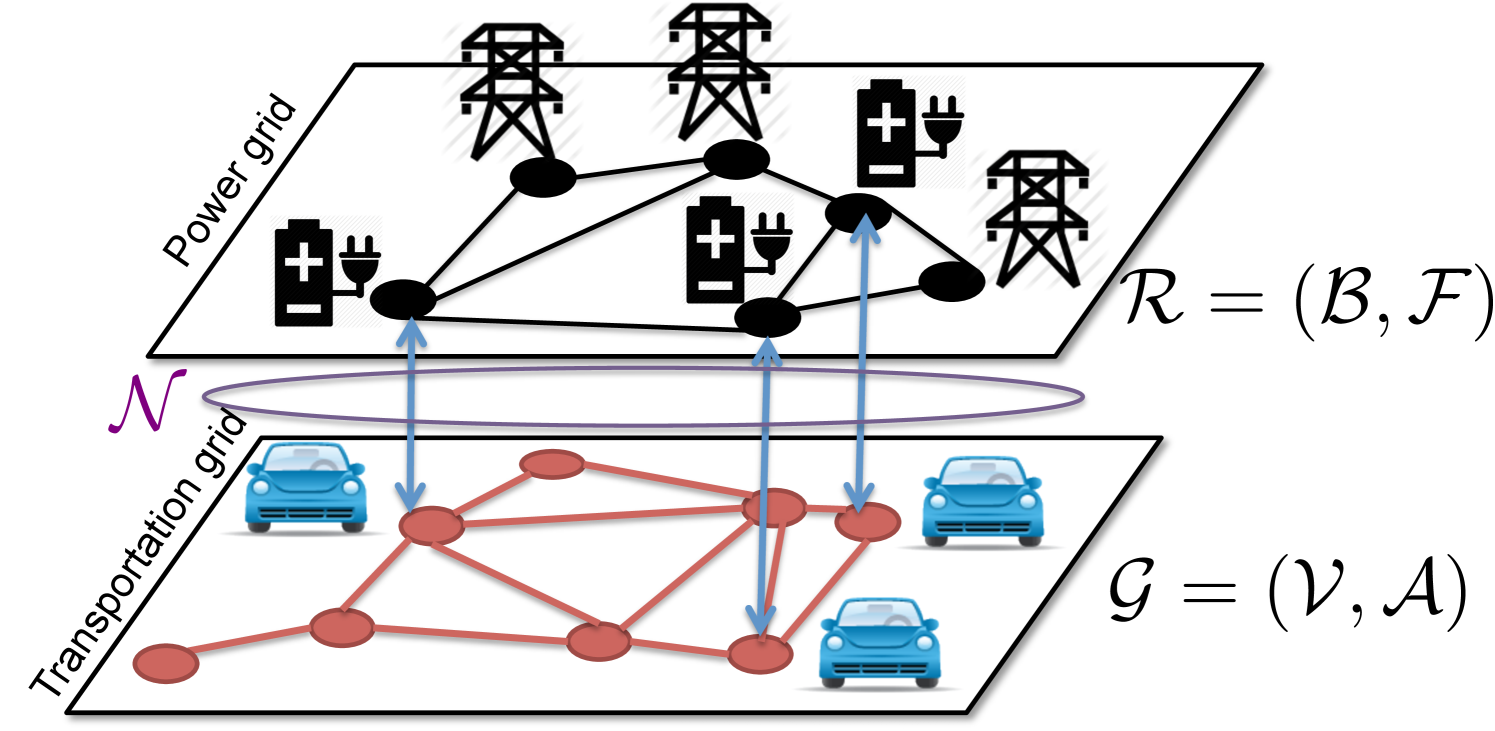
Large-scale adaptation of Electric Vehicles (EV) will affect the operation of two cyber-physical networks: power and transportation systems [1]. Each of these systems has been the subject of decades of engineering research. However, in this work, we argue that the introduction of EVs will couple the operation of these two critical infrastructures. We show that ignoring this interconnection and assuming that the location of EV plug-in events follows an independent process that does not get affected by electricity prices can lead to instabilities in electricity pricing mechanisms, power delivery, and traffic distribution. Hence, we propose control schemes that acknowledge this interconnection and move both infrastructures towards optimal and reliable operation.
To achieve this goal, we show that an individual driver’s joint charge and path decision problem can be modeled as a shortest path problem on an extended transportation graph with virtual arcs. We use this extended graph to study the collective result of all drivers making cost-minimizing charge and path decisions on power and transportation systems. We then show that two non-profit entities referred to as the independent power system operator (IPSO) and independent transportation system operator (ITSO) can collaborate to find jointly optimal electricity prices, charging station mark-ups, and road tolls, while keeping the data of each system private. We show that this collaboration is necessary for correct price design. We further study the generation reserve requirements to operate the grid in the absence of such collaboration.
Prior Art
The study of mechanisms for coping with demand stochasticity and grid congestion is at the core of power systems research. In particular, EVs are acknowledged to be one of the primary focuses of demand response (DR) programs. DR enables electricity demand to become a control asset for the IPSO. For example, the authors in [2, 3, 4, 5, 6, 7, 8, 9, 10, 11, 12, 13, 14, 15, 16, 17, 18], and many others, have proposed control schemes to manipulate EV charging load using various tools, e.g., heuristic or optimal control, and towards different objectives, e.g., ancillary service provision, peak shaving, load following. However, a common feature in [2, 3, 4, 5, 6, 7, 8, 9, 10, 11, 12, 13, 14, 15, 16, 17, 18] is that the location and time of plug in for each request is considered an exogenous process and is not explicitly modeled. Very few works have considered the fact that, unlike all other electric loads, EVs are mobile, and hence may choose to receive charge at different nodes of the grid following economic preferences and travel constraints. This capability was considered in [19, 20] in the problem of routing EV drivers to the optimal nearby charging station after they announce their need to charge. The authors in [21] consider the case where the operator tracks the mobility of large fleets of EVs and their energy consumption and designs optimal multi-period Vehicle-to-Grid strategies. Here we do not consider the case of fleets and look at a large population of heterogeneous privately-owned EVs.
Traffic engineering studies mechanisms for coping with road congestion in the transportation network. At the individual user level, travel paths are planned to avoid congestion as much as possible, naturally leading to shortest path problems [22, 23]. When studying the collective actions of users, the so-called Traffic Assignment Problem is concerned with the effect of individuals’ selection of routes on the society’s welfare, and studies control strategies to guide the selfish user equilibrium towards a social optimum, e.g., [24], [25].
Recently, a line of research has emerged to study the effect of EVs on transportation systems. For example, [26, 27, 28] look at the individual path planning problem by minimizing the energy consumption of EVs, leading to a constrained shortest path problem. However, the interactions with the power grid are not modeled. At the system-level, [29, 30] study efficient solutions for characterizing the redistribution of traffic due to the charge requirements of EVs (paths are forbidden if not enough charge is received to travel them). In contrast to our work, in [29, 30], electricity prices are respectively not considered and taken as given. Accordingly, these works are complementary to ours and do not address the electricity price design aspect that we are interested in (more details in Remark III.3). To the best of our knowledge, the only work that considers price design is [31]. In [31], charge is wirelessly delivered to EVs while traveling. Hence, EVs can never run out of charge. The authors show that if a government agency controls the operations of both the transportation and power networks or can design tolls as a decentralized control measure, the effect of EVs on the grid can be optimized by affecting the drivers’ choice of route. In spite of a somewhat similar set up, [31] and our work have major differences: 1) Our model is different in that we assume EVs make stops at charging stations and the amount of charge received is a choice made by the driver, leading to a different pricing structure, based on the concept of virtual charging arcs; 2) We consider the IPSO and ITSO as two separate entities and look at how they can design prices if they collaborate together with minimal data exchange using the principles of dual decomposition. We also study the adverse effects of the lack of such collaboration; 3) We study how the IPSO can set prices in the absence of such collaboration through procuring generation reserves.
Remark I.1.
To be able to derive analytical results, we have chosen to remain in a static setting. This means that the customers’ travel demand, the baseload, and generation costs are all time-invariant. Our preliminary work published as a conference paper [32] models this problem under a dynamic setting. The main contribution of [32] is proposing the general model of the ESPP and the extended transportation graph. However, the dynamic model studied in [32] in its full generality was not amenable to an analytical characterization of the aggregate control problem and hence could not provide design insights. In contrast, the present work introduces significant simplifications by considering a static setting. The static formulation removes the non-convexity of the problem and allows for a novel analytical treatment.
II Overview
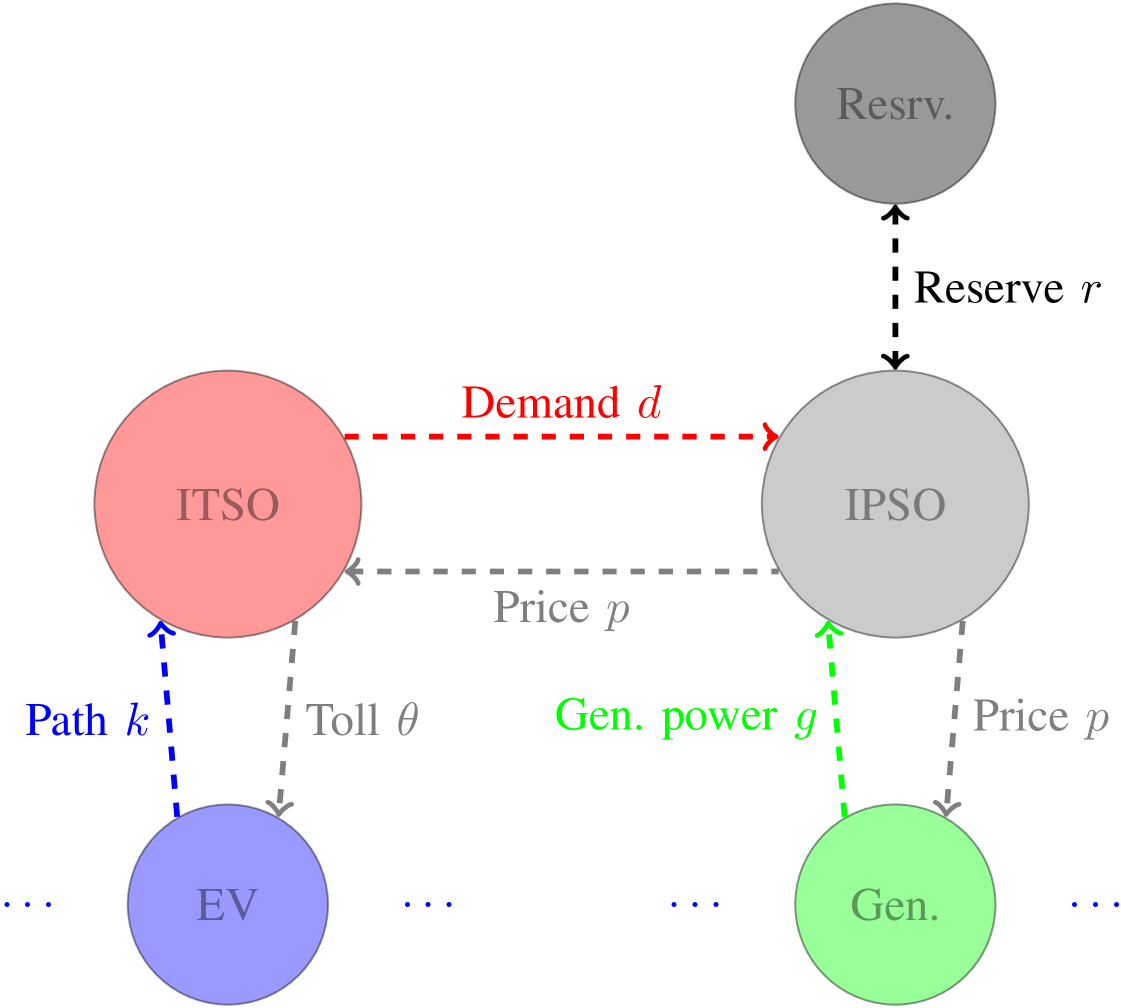
We study a large network of EV and Internal Combustion Engine Vehicles (ICEV) owners that optimize their daily trip costs, including the path they take to complete a trip as well as refueling strategies. A short model of the decision making process by individual EV drivers is first presented in Section III, mainly to introduce the extended transportation graph, a novel concept we use in this paper to integrate individual decisions into system-level control strategies for coupled infrastructures. The extended graph construct captures the fact that EVs’ route and charge decisions are affected by the state of two networks, namely the power and the transportation networks. The transportation network is managed by a non-profit ITSO (red circle in Fig. 2), who knows about the trip patterns of the population and can impose tolls on public roads to affect the individuals’ routing decisions. The power network is managed by a non-profit IPSO (light gray circle), who controls electricity generation costs (green circle) and is in charge of pricing electricity that affect individual EV’s charging decisions. Ideally, we would like to minimize the total transportation delay and electricity generation cost that the society incurs. However, as the IPSO and the ITSO are two separate entities, we study whether they can achieve this goal with or without direct collaboration under various schemes presented in Section IV (and in Fig 5). We numerically study these schemes in Section VI.
III The Individual Driver’s Model
Let us first focus on the decision making process of an individual EV driver (the blue circle in Fig 2). In order to complete a trip, the driver needs to decide on 1) which path to take to get from his origin to the destination; and 2) the locations at which he/she should charge the EV battery and the amount of charge to be received at each location. We model the cost structure associated with these decisions next.
Notation
We use bold lower case to indicate vectors and bold upper case to indicates matrices. The notation indicates that the elements that comprise a column vector or a matrix each correspond to a member of a set . The symbols and denote element-wise and inequalities in vectors. The transpose of a column vector is denoted by . The all one and all zero row vectors of size are denoted by and respectively.
| Set of nodes in the transportation network | ||
| Set of arcs in the transportation network | ||
| Set of nodes with charging facilities | ||
| The transportation graph | ||
| Set of energy-feasible paths that connect the origin and destination for an individual user | ||
| Length of path | ||
| Flow on arc of transportation graph | ||
| Flow into charging station located at node | ||
| Price of electricity at node | ||
| Energy received at node | ||
| Set of possible charging amounts at | ||
| Plug-in fee at node | ||
| Charging rate at node | ||
| Latency function of traveling on arc | ||
| Wait time to be plugged in at node | ||
| Value of time to users | ||
| Cost each user incurs for traveling on arc | ||
| Cost to receive charge of at node | ||
| Energy required to travel arc | ||
| The extended transportation graph | ||
| Set of nodes in | ||
| Set of arcs in | ||
| Set of virtual charging arcs for charging station at node | ||
| Set of all virtual charging station entrance and bypass arcs | ||
| The electricity bill to charge for virtual arc | ||
| Set of different origin-destination clusters | ||
| Set of feasible paths on for cluster | ||
| Rate of EVs in cluster | ||
| rate of cluster EVs that choose path | ||
| Arc-path incidence matrix for cluster | ||
| Vector of generation outputs at all network nodes | ||
| Vector of network generation costs | ||
| Vector of inelastic non-EV demand at all network nodes | ||
| Vector of EV charging demand at all network nodes | ||
| The power transfer distribution matrix | ||
| Line flow limits | ||
| Matrix that maps virtual link flow to power system load | ||
| Auxilary cost function for arc (see (18)) | ||
| Reserve capacity prices at all network nodes | ||
| Reserve capacity prices at all network nodes |
III-A Congestion Costs
We model the transportation network through a connected directional graph , where and respectively denote the set of nodes and arcs of the graph.
Traveling on the transportation network is associated with a cost for the user since he/she values the time spent en route. The time to travel between an origin and a destination node is comprised of the time spent on arcs that connect these two nodes on . Here we adopt the popular Beckmann model for the cost of traveling an arc, i.e., a road section [33]. Accordingly, we assume that the travel time for each arc only depends on the rate of EVs per time unit that travel on the arc, which we refer to as the arc flow and denote by . The time it takes to travel arc is then represented by a latency function , which is convex, continuous, non-negative, and increasing in . The congestion cost that a user incurs for traveling arc is given by:
| (1) |
where is the cost of one unit of time spent en route. Hence, the cost to travel link is:
| (2) |
where corresponds to any tolls that the driver should pay to the ITSO, if any such toll is enforced for link .
Moreover, traveling each arc requires a certain amount of energy (see Fig. 2). Energy needs to be received from the power grid and stored in the EV battery. The cost that the user incurs to receive battery charge is modeled next.
III-B Charging Costs
A subset of nodes on the transportation network are equipped with battery charging facilities and, hence, the EV drivers have the choice of charging their batteries at these locations. Naturally, to be able to provide charging services, the nodes are also a subset of the nodes that constitute the power grid graph . Each node has an associated price for electricity . Consequently, if the EV driver chooses to charge at location , he/she will pay:
| (3) |
where is the battery charge amount received at chosen from a finite set , and corresponds to a one-time plug-in fee for the charging station at . Moreover, if is not the origin of the trip, the driver needs to spend some extra time en route in order to receive charge at . This is due to any congestion at the fast charging stations (FCS) plus the time it takes to receive charge. Hence, an extra inconvenience cost is incurred. If the charging rate at FCS is , and the rate of EVs being plugged in for charge at this location is denoted by , this cost is equal to:
| (4) |
where denotes the wait time due to congestion, and is a soft cost model to capture limited station capacity.
III-C The Extended Transportation Graph with Virtual Arcs
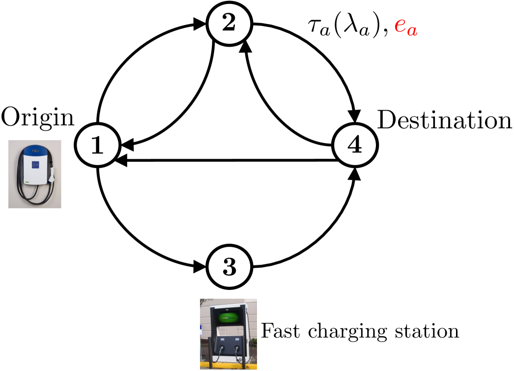
The EV driver’s goal would be to find the least cost path that connects the origin and the destination on the transportation graph while making sure that the EV battery never runs out of charge111Note that with the cost structure we have defined, the EV driver will reach the destination with minimum-possible leftover charge. An extension of the analytical framework to include the value of leftover charge at the destination in the optimization is trivial and has been removed for brevity of notation. We refer the reader to our conference paper [32] for this extension..
Here we show that we can recast the EV driver’s route and charge problem as a resource-constrained shortest path problem on a new extended transportation multigraph . This definition will help us study and control the aggregate effect of individual EVs on power and transportation systems.
Definition III.1.
A travel path on the graph is characterized by an ordered sequence of arc indices where the head node of is identical to the tail node of for all . The length of path is . Alternatively, if is simple, path can be written as an ordered sequence of node indices (excluding the destination node). We further denote a vector of previously defined quantities associated with the arcs using subscripts, e.g., and respectively denote the vectors of charge amounts and travel time required to travel each arc on path .
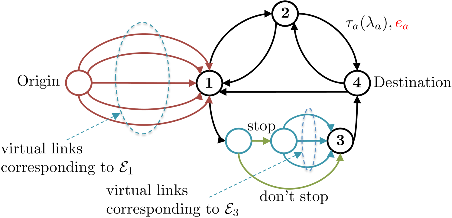
To complete a trip, the driver incurs two forms of costs: the cost associated with arcs and the cost associated with the charging decisions taken at nodes. However, we can observe charging is very similar in nature to traveling: 1) it takes a certain amount of time (due to both charging rate limitations and congestion); 2) it has a cost; and 3) it changes the energy level of the battery. Acknowledging this similarity, we transform the EV driver’s decision problem to a shortest path problem by associating charging decisions made at the nodes of the transportation graph to a set of new virtual arcs to be added at each node where charging is possible. At each origin and destination node where charging is possible, the following transformation would capture all decisions:
-
•
The decision of how much to charge: a set of virtual arcs added at node are each associated with a specific choice of how much to charge, i.e., . Hence, the energy gained by traveling each new virtual arc is set to be one such member of (red arcs in Fig. 4). Equivalently, we can say that the energy required to travel the virtual arc is negative. Travel time is .
At the FCS, these transformations capture all decisions:
-
•
The decision to stop or skip stopping at a charge station en route: the driver can either take a charging station entrance arc (labeled “stop” in Fig 3) and plug in their EV at the station, or skip stopping at the station via a bypass arc with zero travel time and energy requirements (green arcs in Fig. 3). Charging station entrance arcs can be congested;
-
•
The decision of how much to charge if stopping at : the charging station entrance arc is connected in series to a set of virtual arcs capturing the choice of amount of charge (blue arcs in Fig. 3).
The flow on the charging station entrance arc will capture the wait time to be plugged in at the station. The set of all entrance and bypass arcs for all charging stations is . The new extended transportation graph with these virtual arcs would then have the following set of arcs:
Consequently, the transformed problem seeks a shortest path on this extended graph from the origin to the destination, with the cost of traveling each arc being the sum of its travel time cost and all monetary charges such as the electricity bill or tolls. The travel time costs on is given by:
| (5) |
All other monetary costs can be captured as:
| (6) |
and hence, each driver selfishly optimizes their trip plan by solving the Energy-aware Shortest Path Problem (ESPP):
| (7) |
where is now the set of energy-feasible paths that connect the origin and the destination on the extended graph . Energy-feasibility of a path ensures that the battery will never run out of charge en route. Next, we define energy-feasibility mathematically.
Definition III.2.
A path is energy-feasible on iff :
These two constraints ensure that the EV never runs out of charge en route if taking path , and that the battery charge state never exceeds battery capacity. A vector of dimension zero is simply empty. Note that with this definition, we can determine whether a path is energy-feasible independently of the network congestion mirrored through . Hence, for system-level control of , the set of energy-feasible paths can be calculated offline.
Remark III.3.
The ESPP (7) can be solved using Dynamic Programming (DP) algorithms with pseudo-polynomial complexity [34]. Polynomial-time Dijkstra-like algorithms for solving the shortest path problem cannot be applied due to the existence of the energy-feasibility constraint (see [26, 35]). This is mainly because the cost of a path is no longer just the sum of its arc costs (as energy constraints cannot be attributed to individual arcs but a sum over multiple arcs). Proposing efficient solution methods for the ESPP is beyond the scope of this paper. Instead, our focus is to use the extended graph to study aggregate control strategies. We refer the reader to recent papers studying efficient solutions and search heuristics for variations of ESPP, e.g., [30, 36, 37, 38]. For our small numerical experiment, we use a brute force approach to enumerate all loop-free energy-feasible paths for all origin-destination pairs on the extended transportation graph, as often done in the transportation literature. While for our small experiment the complexity of this approach does not pose a computational challenge, in more realistic models this is an issue that needs to be properly addressed to allow scalability. We will consider this issue as part of our future work.
Now, imagine that every EV owner in the society solved (7) to plan their trips. These users share two infrastructures: the transportation network, and the power grid. Hence, collectively, EVs give rise to a traffic and load pattern, determining which roads and grid buses are congested and hence, will have longer travel times and higher electricity prices. Through this interaction, individuals affect each other’s cost, leading to the system-level problem that we are interested in.
IV System Level Model
At the system level, the extended transportation graph helps us study the collective effect of individual drivers on traffic and energy loads as a network flow problem. Here virtual arcs are added at all potential origins and FCSs.
At the aggregate level, the system variables, i.e., the flow rate of vehicles on arcs , the price of electricity , and the tolls can no longer be considered as variables imposed upon the system but rather as variables to be jointly optimized by system operators.
If a single entity was in charge of monitoring the state of both networks and controlling all EVs’ charge and route decisions, they can maximize the social welfare by solving for the optimum route and charge plan for each individual such the the total transportation congestion and generation costs that the society incurs is minimized. In doing so, this entity needs to ensure that the constraints of the transportation and power systems are not violated. The power system’s constraints ensure the balance of supply and demand in the grid and that the physical limits of transmission lines are not violated. The transportation system constraints ensure that every driver will be able to finish their travel.
In reality, power and transportation systems are operated by the IPSO and the ITSO respectively, and their operational data is not shared. The IPSO is in charge of optimizing generation costs subject to power system constraints, and the ITSO is in charge of optimizing transportation costs subject to transportation system constraints. Also, individuals’ route and charge decisions can only be affected through prices. We first study the ITSO and IPSO strategies separately in Subsections IV-A and IV-B and their optimal pricing. Then we look at how they interact (and possibly achieve the socially optimal outcome) in Section V.
IV-A The ITSO’s Charge and Traffic Assignment Problem
We assume that drivers belong to a finite number of classes . Vehicles in the same class share the same origin and destination. Vehicles could include both EVs as well as ICEVs. A given class q would contain either EVs or ICEVs but not both. Drivers of the same class are represented by a set of feasible paths , each of which allows them to to finish their trip on the extended graph. For EVs, this is equivalent to the set of energy-feasible paths given in Definition II.2 and can be enumerated offline for each class. For ICEVs, we can assume these paths simply include transportation arcs in that connect the origin and destination, and do not enter charging stations. Clearly, any other path selection method that considers more realistic constraints can also be applied. We leave the study of optimal clustering mechanisms that assign heterogeneous users to a finite of number of classes to future work.
Each customer directly affects the flow of the arcs that constitute his/her path. To model this effect, we define:
-
•
as the travel demand rate (flow) of EVs in cluster . This demand is taken as deterministic and given;
-
•
as the rate of cluster EVs that choose path . We define .
Naturally, since every driver has to pick one path, the following conservation rule holds:
| (8) |
Given the path decisions of all EV drivers, i.e., the ’s, the flow of EVs on arc is given by , where is an arc-path incidence indicator (1 if arc is on path and 0 otherwise). This is written in matrix form as:
| (9) |
where denotes the vector of network flows and is a matrix such that .
The flow on the virtual arcs of the extended graph leads to a power load. We denote the charging demand at each node of the grid as a vector , given by:
| (10) |
where is a matrix given by:
| (11) |
Let . If an ITSO is in charge of determining the optimal path and charge schedule for each EV such that the aggregate cost is minimized, it can solve a modified version of the classic static traffic assignment problem [39] on the extended graph, which we refer to as the charge and traffic assignment problem (CTAP):
| (12) | ||||
where .
IV-B The IPSO’s Economic Dispatch Problem
To serve the charging demand of EVs, a set of generators are located at different nodes of the power network . For brevity, let us assume that a single merged generator is located at each node of the grid. Assuming that the generation at each node is denoted by a vector and the baseload (any load that does not serve EVs) by a vector , there are three constraints that define a feasible generation mix in the power grid. First of all, must be within the capacity range of the generator at node , i.e., . Second, the demand/supply balance requirement of the power grid should be met, i.e.,
| (13) |
Third and last, the transmission line flow constraints of the grid under the DC approximation [40] translate into:
| (14) |
where the matrix is the power transfer distribution matrix of the grid, explicitly defined in [40], and is a vector containing arc (line) flow limits (in both directions).
In most power grids, one such feasible generation mix is picked by an IPSO to serve demand. We assume that at least one feasible generation mix always exists for every possible load profile. The IPSO’s objective is to pick the cheapest feasible generation mix. Let us denote the cost of generating units of energy at node as a strongly convex and continuous function , and the vector of generation costs as . Given a demand from EVs, the IPSO solves an economic dispatch problem to decide the optimal generation dispatch [41]:
| (15) | ||||
Note that the optimal traffic and generation schedules determined through (12) and (15) minimize the total cost to society. However, they do not necessarily minimize the cost of each individual entity that is involved, e.g., the EV drivers or the generators. Hence, one cannot merely ask these selfish users to stick to the socially optimal schedule. An economic mechanism is necessary to align selfish behavior with socially optimal resource consumption behavior. The use of pricing mechanisms is a way of achieving this goal in a distributed and incentive-compatible fashion. We highlight pricing mechanisms that can be used for (12) and (15) next.
IV-C Pricing Mechanism for Electric Power
To incentivize profit-maximizing generators to produce at an output level , we apply the principle of marginal cost pricing. The principle states that the electricity price at node , i.e., , must satisfy:
| (16) |
Let us introduce Lagrange multipliers and respectively for the balance and line flow constraints in (15). Writing the KKT stationarity condition for (15) then leads to:
| (17) |
commonly referred to as Locational Marginal Prices (LMP) in the power system literature. The reader should note that this is the same price vector that is fed into the ITSO optimization (12) and would affect the charging demand at different nodes of the grid, i.e., in (15), which would in turn affect the price again. This feedback loop highlights the coupling between smart power and transportation systems that we are interested in, further studied in Section V.
IV-D Tolls to Align Selfish User Behavior with Social Optimum
In the transportation network, if every user solves an ESPP given in (7) and no tolls are imposed by the ITSO (), the aggregate flow would be determined based on a state of user-equilibrium. This user equilibrium flow is most likely not equivalent to the social optimal flow in (12). To mathematically characterize this equilibrium, define an auxilary modified cost function for the extended transportation graph’s arcs as:
| (18) |
with and given by (5) and (11). Moreover, let . Then, according to the well-known Wardrop’s first principle [42], the user equilibrium flow would be the solution of the optimization problem:
| (19) | ||||
| s.t.Constraints in (12) |
So how can the ITSO get the individual drivers to follow the socially optimal flow calculated in (12)? We present the answer in Theorem IV.1.
Theorem IV.1.
(Marginal congestion pricing) The aggregate effect of individual route and charge decisions made by EV drivers, i.e., the solution of (19), will be equivalent to the optimal social charge and route decision in (12) iff the ITSO imposes a toll at each arc of the extended graph equal to the externality introduced by each user that travels the arc on the other users’ costs, i.e.,
| (20) |
Proof.
Remark IV.2.
(Congestion Mark-up at Charging Stations) The arc toll on the virtual charging station entrance arcs would correspond to a congestion mark-up (plug-in fee) for all EVs stopping at each station. This captures the user externality introduced by limited charging station capacity. The spots at FCSs located at busy streets and highways or ones that allow a user to take less congested routes are coveted by many drivers and thus have higher plug-in fees.
V Interactive Network Operation
For scalability reasons, the IPSO cannot be expected to consider detailed models of the transportation system demand flexibility when calculating the prices . However, we next show that completely ignoring the interconnection between the two infrastructures (the status-quo) can have adverse effects on both infrastructures. This motivates us to introduce a collaborative pricing scheme using dual decomposition. The schemes we study for interactions between the IPSO and ITSO towards network operation are highlighted in Fig. 5.
V-A Greedy pricing
Let us look at the scenario that would happen if no corrective action is taken in regards to how the grid is operated today and hence, smart transportation and energy systems are operated separately. In this disjoint model, the IPSO ignores the fact that the load due to EV charge requests can move from one grid bus to another in response to posted prices. Instead, LMPs are designed assuming that charge events will happen exactly as in the last period (this could be the previous day, the average of the previous month, etc.). On the other hand, the ITSO ignores the effect of EV charge requests on electricity prices, and takes electricity prices as a given when designing road and FCS congestion tolls.
Claim: Under this greedy pricing scheme, the congestion and electricity prices and could oscillate indefinitely.
We substantiate this claim through a numerical example in Section VI. This, along with the loss of welfare experienced when our infrastructure is operated at a suboptimal state, motivates us to look into schemes which can allow the ITSO and IPSO to operate their networks optimally and reliably.
V-B Collaborative pricing
Proposition V.1.
An efficient market clearing LMP can be posted through a ex-ante collaboration between the IPSO and ITSO following a dual decomposition algorithm.
Proof.
A market clearing price is efficient (maximizes social welfare) if the flow and generation values and are the solution of:
| (22) |

The last two constraints contain both decision variables and couple the IPSO and ITSO optimization problems. Let us introduce Lagrange multipliers and respectively for the balance and line flow constraints. The partial Lagrangian of (22) considering only the coupling constraints is:
| (23) |
with . Since is separable, we can minimize over and in two separate subproblems, allowing us to use standard dual decomposition with projected subgradient methods to find the optimal price. Consider a sequence and of Lagrange multipliers generated by the iterative decomposition scheme. Then, at the -th iteration, the ITSO solves for the optimal extended graph flow through a subproblem that has the same structure as (12), with electricity prices at iteration , , set as:
| (24) |
On the other hand, the subproblem solved by the IPSO is:
| (25) | ||||
The IPSO then updates the balance and congestion components of the LMP, i.e., and , through:
| (26) |
V-C Optimal reserve capacity for trial-and-error pricing
In theory, the above algorithm can eliminate the need for the existence of an ex-ante222The term ex-ante refers to actions that are adjusted as a result of forecasting user behavior and not actual observations, while ex-post refers to actions that are based on actual observations rather than forecasts. ITSO collaboration for calculating electricity prices. Instead, imagine that the IPSO can actually post electricity prices according to (26) and gradually find the optimal market clearing LMP by observing the charging demand of the actual transportation system333Note that this is only possible if the time-scale at which the network flow reaches its new equilibrium in response to new posted prices and tolls is much smaller that the time-scale at which electricity costs or travel demands change.. When dealing with unknown demand functions in commodity pricing, this is referred to as the trial-and-error approach, see, e.g., [44], for prior use of such approaches in toll design.
Implementing this approach has two requirements:
1) The IPSO should be willing to move away from the greedy pricing scheme in order to eventually maximize societal welfare (even though the extra welfare generated might not be easily quantifiable and the operating point might not correspond to minimum generation costs);
2) More importantly, primal feasibility is most likely violated when using Lagrangian relaxation to handle coupling constraints in (22). This means that when posting prices according to (26), the IPSO should expect the balance and flow constraints to be violated in order for the algorithm to converge, and plan accordingly. In power grids, any unpredictable violation of reliable system operation is referred to as a contingency (a threat to the security of the system) and is handled through generation reserves.
Definition V.2.
(Reserves) In power grids, a generation reserve capacity of allows the IPSO to compensate for any demand-supply imbalances after market clearing as long as , or equivalently . This is typically done by adjusting the output of an already online generator either upward or downward. Given a reserve capacity of , the balance equation will become:
| (27) |
where can be chosen at the IPSO’s discretion after observing the demand . The reserve capacity should be procured in advance.
Note that the dispatched reserve generation affects the line flows and hence the flow constraint becomes:
| (28) |
Here we will use bounds on primal infeasibility to determine the reserve capacity that needs to be procured by the IPSO in this type of ex-post LMP adjustment. For simplicity, we consider a constant step size rule such that for all . Note that in this scheme, after each price adjustment iteration , the approximate primal solutions, which are the last iterate and , are actually implemented. Assume that the IPSO knows that during the -th iteration,
| (29) |
where . For dual first order algorithms such as dual gradient and dual fast gradient methods (any of which can be employed by the IPSO for price update), such bounds were recently provided by [45]. For example, for dual gradient methods, one possible bound is given by:
| (30) |
where and is the Lipschitz constant for the dual problem of (22). We now need to show that the bound in (30) is well-defined.
Lemma V.3.
The dual problem of (22) has finite Lipschitz constant and bounded optimal dual variables, i.e., and .
Proof.
The finiteness of is a consequence of the strong convexity of the objective function444Recall that is non-negative, convex and increasing (cf. (1)), therefore the product is strongly convex. of (22) [45]. Furthermore, we see that (22) is a convex problem with linear inequality constraints and its optimal objective value is finite (as we have assumed that at least one feasible generation mix exists for every possible load profile). Consequently, strong duality holds for (22) and there exists a set of bounded optimal dual variables. ∎
To calculate (30), the IPSO has to access to the set of potentially optimal energy and congestion prices and . Without access to travel patterns, an estimate of the upper bound to can be evaluated using many methods. For example, we can calculate these bounds by a) performing Monte-Carlo simulations by setting to different values between its upper and lower bounds given the limited capacity of charging stations (charging stations operating anywhere until full capacity) [46]; b) studying critical load levels as suggested in [47]; c) solving a Mathematical Program with Equilibrium Constraints (MPEC) [48]. We chose to solve an MPEC to find this bound; see Appendix A.
Given (29), the IPSO needs to ensure that (27) and (28) hold by appropriately choosing a reserve capacity to be procured for each future to ensure system security.
Proposition V.4.
(Security-Constrained Ex-post Price Adjustments) Given unit reserve capacity prices at each node of the power grid for iteration , the optimal reserve capacity to be procured at different grid buses for iteration of the price adjustment algorithm is given by:
| (31) | ||||
where the constraint is a piecewise-linear function of , and the numbers are given.
Proof.
The optimal reserve capacity is equal to the cheapest possible nodal reserve capacity combination that can restore the network balance and flow constraints under any possible amount of feasibility violation specified in (29), i.e., we have the following robust optimization problem:
| (32) | |||
where and
where and denotes the minimum/maximum possible . Problem (32) is equivalent to:
| (33) | ||||
where
| (34) | ||||
| s.t. | ||||
If is feasible, its dual problem is bounded and the dual optimum will be 0. Thus, we can write (33) as:
| (35) | ||||
where
| (36) | ||||
Since , this is equivalent to:
| (37) | ||||
Note that is neither convex nor concave in and (bilinear). The constraint set is a polyhedron and hence, the optimal solution of is one of the extreme points of the polyhedrons and . This shows that the constraint is a convex piecewise linear function in . ∎
Remark V.5.
In general, we have no knowledge of the extreme points of and , and computing is non-trivial. Hence, proper approximation algorithms need to be studied for solving (31). However, this is out of the scope of this paper. See [49] for the treatment of a somewhat similar problem, where the use of an outer approximation algorithm is proposed. Instead, in our numerical results, we resort to a sample/scenario-approximation method [50, Chapter 2.6]. For example, we replace the set by a finite set . In this case, (37) will be turned into a convex program with a finite number of linear inequalities.
VI Numerical Examples
This section investigates the need for the joint EV management scheme we propose through numerical analysis of system performance. We focus on the system level optimization. We assume that charging stations are publicly owned infrastructure for the sake of simplicity. This means that we assume electricity is sold at wholesale prices to EV drivers555In reality, EV drivers may purchase flat rate charging services from for-profit entities that trade with the wholesale market and can use appropriate economic incentives (similar to the tolls discussed in this paper) and recommendation systems to guide the customers towards optimal stations. This is beyond the scope of this work..
The transportation network is shown in Fig. 6. For each arc (road section), we define the latency function as:
| (38) |
where is the minimum time required to travel through arc . We set for the cost spent en route. Note that this might seem like a rather low number but it would be scaled up by a factor of 10 if electricity is traded at retail prices instead of wholesale. The power network is modeled using the line and generation cost parameters of the IEEE 9-bus test case, except that several more buses are modeled as load buses where EVs can charge; also see Fig. 6.
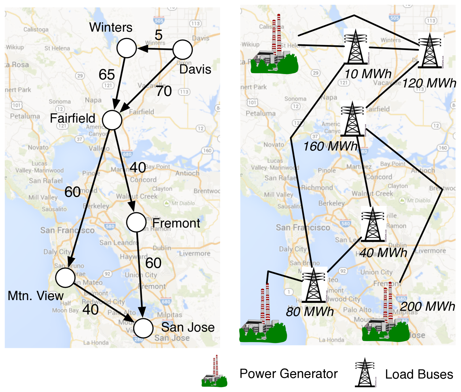
The intermediate nodes, i.e., Winters, Fairfield, Mountain View and Fremont, are equipped with an FCS. Each FCS is capable of supplying 1 kWh to an EV every 5 minutes, and the available charging options are kWh (the same charging options hold for the origin). It is assumed that each EV consumes 1 kWh of energy to travel 25 miles, and the battery capacity is 6 kWh for all EVs. There are two O-D pairs considered in the network. Specifically, of the drivers are traveling from Davis, CA to Mountain View, CA; and of the drivers are traveling from Davis to San Jose, CA. At the origin, i.e., Davis, the EVs have an initial charge of 4 kWh. As such, there are classes of users.
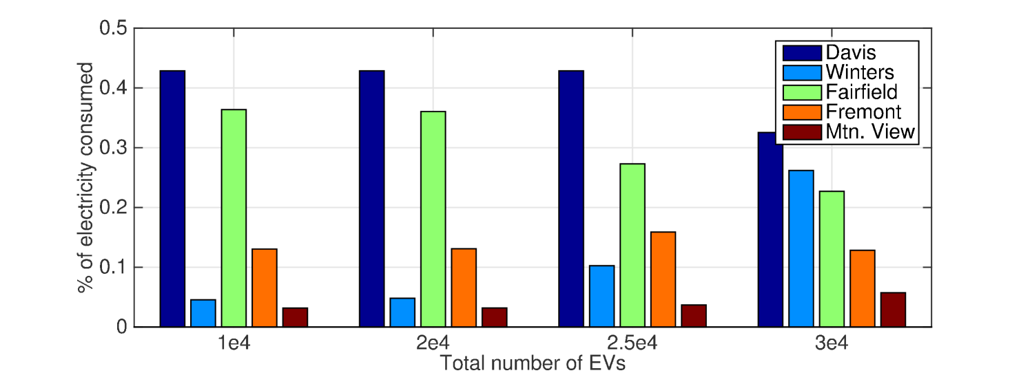
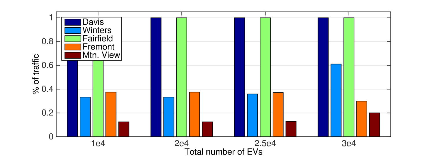
In the first numerical example, we study how the total number of EVs can affect the IPSO/ITSO’s decision. We assume full IPSO/ITSO cooperation such that the social optimal problem (22) can be exactly solved. As seen in Fig. 7, the traffic pattern changes as we gradually increase the total number of EVs per epoch. For instance, more EVs are routed through Winters, instead of going to Fairfield from Davis directly; similar observations are also made for the Fairfield-Mountain View-San Jose path. This is due to the fact that the power/transportation network has become more congested, leading to a different traffic pattern.
Our next step is to study the scenario with ex-ante IPSO/ITSO cooperation. We compare the myopic pricing scheme to the dual decomposition approach. The first task is to investigate the behavior of the system under the myopic pricing scheme. The total number of EVs is fixed at per epoch. In this case, we initialize the electricity price at each site at per MWh to solve (12). The traffic pattern against iteration number of this disjoint optimization is shown in Table II. We observe that the system oscillates between two traffic patterns, one having the lower average traveling time and the other one with a lower electricity cost. As described in Section V-A, this oscillation behavior is due to the lack of cooperation between the IPSO and ITSO. We see that at iteration , the electricity prices are the same across the charging stations, therefore the ITSO assigns the traffic by simply minimizing the travel time. This decision, however, leads to an uneven distribution in energy consumption across the power network . At iteration , the IPSO lowers the electricity price at Winters; and increases the price at Fairfield, Fremont and Mountain View. This motivates the ITSO to re-assign the traffic pattern.
An interesting point to note is that the disjoint optimization may even lead to an infeasible IPSO decision when the total number of EVs considered is large. This is an extreme case of the example considered in Table I. In this case, the inability of the greedy pricing method to correctly model the response of the EV population to posted prices would result in an unsafe increase of load at locations where the grid is congested and hence the load needs to be shed to keep transmission lines as well as transformers safe.
| SO | DO () | DO () | |
|---|---|---|---|
| Davis | 67.80 MWh | 67.80 MWh | 67.80 MWh |
| @$57.38/MWh | @$57.38/MWh | @$58.04/MWh | |
| Winters | 12.56 MWh | 7.227 MWh | 15.87 MWh |
| @$57.38/MWh | @$57.38/MWh | @$54.50/MWh | |
| Fairfield | 49.88 MWh | 57.32 MWh | 43.52 MWh |
| @$57.38/MWh | @$57.38/MWh | @$66.59/MWh | |
| Fremont | 22.56 MWh | 20.83 MWh | 25.23 MWh |
| @$57.38/MWh | @$57.38/MWh | @$65.09/MWh | |
| Mtn. View | 5.392 MWh | 5.031 MWh | 5,781 MWh |
| @$57.38/MWh | @$57.38/MWh | @$61.73/MWh | |
| Fr. Winters | 7,533 | 7,534 | 7,936 |
| Fr. Fremont | 8,475 | 8,409 | 9,375 |
| Fr. Mtn View | 2,825 | 2,825 | 3,125 |
| Travel time | 188.36 min. | 188.36 min. | 188.39 min. |
| Objective | $30,332.55 | $30,364.61 | $30,333.06 |
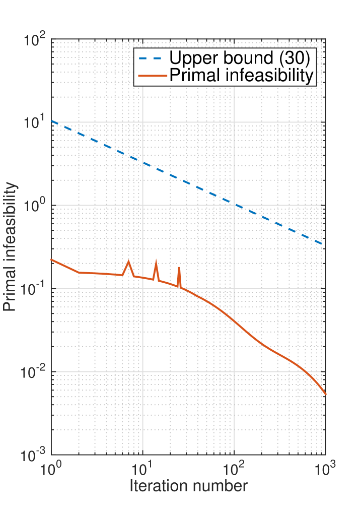
The above example demonstrates that applying myopic pricing may result in an unstable system. Next, we investigate the performance of the dual decomposition algorithm (cf. Proposition V.1), which describes a systematic method for cooperation between the IPSO and ITSO. Here, the total number of EVs is fixed at per epoch. The dual decomposition is initialized by setting and . As the dual decomposition algorithm is known to converge to the social optimum, we are interested in studying its convergence speed with the violation in infeasibility. We set the step size as for all and apply the algorithm on the same scenario as before. For the constant in (30), we upper bound it by solving an MPEC using an approach similar to [48].
We compare both infeasibility measures against the iteration number in Fig. 8 (Left). We can see that the dual decomposition algorithm converges in approximately iterations, and it returns a solution that is approximately feasible. We observe a decaying trend with the actual infeasibility.
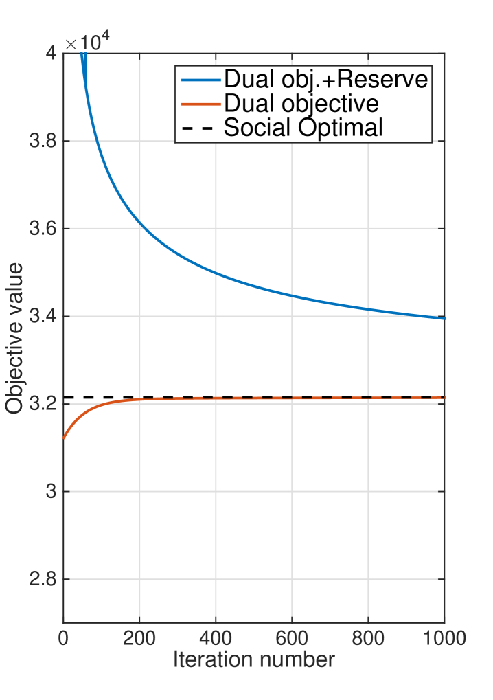
Lastly, we study the effects of ex-post IPSO price adjustment based on the estimated in (30). The reserve procurement problem (31) is approximated using a sample-approximation method, where the candidate points for are selected randomly within the bound . We assume that the reserve capacity is purchased at a price of per MWh at all sites. Here, an interesting comparison is the overall cost needed to purchase such reserve capacity and the cost to operate the system under (the estimated) infeasibility, i.e., the dual objective value. The overall cost is shown in Fig. 8 (Right) as ‘Dual obj.+Reserve Cost’. We observe that such cost is always higher than the social optimum cost due to a possible mismatch between the electricity cost per unit in purchasing the reserve capacity; yet the difference decreases as the iteration number grows.
VII Conclusions and Future Work
The implications of large-scale integration of EVs on power and transportation networks, leading to an interdependency between the two infrastructures, were studied under a static setting. We saw that a collaboration between the IPSO and the ITSO can lead EVs towards a socially optimal traffic pattern and energy footprint, and highlighted the adverse effects of ignoring the interconnection between the two infrastructures. We further analyzed the reserve capacity requirements of operating the grid without a direct collaboration between the IPSO and ITSO. These results were obtained under an ideal static setting and in the absence of retail markets. Important issues remain to be studied in future work. For example, EV charging facilities are expected to be privately-owned, and hence pricing decisions would be left to profit-maximizing entities competing against each other to attract EV drivers to their station. This would affect the IPSO’s ability to impose taxes on many arcs in the extended transportation graph and would lower the IPSO’s ability to maximize social welfare. The impact of hourly dynamics of electricity prices and travel patterns is another important aspect that requires further analysis. In this case, non-convexities of the dynamic traffic assignment problem would extend to the IPSO’s price design problem.
Appendix A MPEC for finding in (30)
To compute the bound (30), we need an upper bound on . To calculate such a bound, we use an MPEC to enumerate all the possible EV demand valus and their corresponding optimal dual variables :
where are lower/upper bounds to the electricity demand requested by the EVs and is a regularization parameter for the power generation constraints. As seen in (17), the lower-level minimization problem finds the optimal dispatch and hence the optimal dual variables for each of the possible demand profiles .
References
- [1] M. Kezunovic, S. Waller, and I. Damnjanovic, “Framework for studying emerging policy issues associated with phevs in managing coupled power and transportation systems,” in 2010 IEEE Green Technologies Conference, April 2010, pp. 1–8.
- [2] A. Saber and G. Venayagamoorthy, “Efficient utilization of renewable energy sources by gridable vehicles in cyber-physical energy systems,” Systems Journal, IEEE, vol. 4, no. 3, pp. 285–294, 2010.
- [3] M. Erol-Kantarci and H. Mouftah, “Management of phev batteries in the smart grid: Towards a cyber-physical power infrastructure,” in 7th IWCMC, 2011, pp. 795–800.
- [4] Z. Ma, D. Callaway, and I. Hiskens, “Optimal charging control for plug-in electric vehicles,” in Control and Optimization Methods for Electric Smart Grids. Springer New York, 2012, vol. 3, pp. 259–273.
- [5] Y. Xu and F. Pan, “Scheduling for charging plug-in hybrid electric vehicles,” in Decision and Control (CDC), 2012 IEEE 51st Annual Conference on, Dec., pp. 2495–2501.
- [6] S. Chen, Y. Ji, and L. Tong, “Deadline scheduling for large scale charging of electric vehicles with renewable energy,” in Sensor Array and Multichannel Signal Processing Workshop (SAM), 2012 IEEE 7th, June, pp. 13–16.
- [7] S. Han, S. Han, and K. Sezaki, “Development of an optimal vehicle-to-grid aggregator for frequency regulation,” Smart Grid, IEEE Transactions on, vol. 1, no. 1, pp. 65–72, June.
- [8] S. Chen, T. Mount, and L. Tong, “Optimizing operations for large scale charging of electric vehicles,” 2013 46th Hawaii International Conference on System Sciences, vol. 0, pp. 2319–2326, 2013.
- [9] O. Sundstrom and C. Binding, “Planning electric-drive vehicle charging under constrained grid conditions,” in International Conference on Power System Technology (POWERCON), 2010, pp. 1–6.
- [10] M. Caramanis and J. M. Foster, “Management of electric vehicle charging to mitigate renewable generation intermittency and distribution network congestion,” in IEEE Conference on Decision and Control. Ieee, 2009, pp. 4717–4722.
- [11] K. Mets, T. Verschueren, W. Haerick, C. Develder, and F. De Turck, “Optimizing smart energy control strategies for plug-in hybrid electric vehicle charging,” in IEEE/IFIP Network Operations and Management Symposium Workshops, 2010, pp. 293–299.
- [12] S. Deilami, A. Masoum, P. Moses, and M. A. S. Masoum, “Real-time coordination of plug-in electric vehicle charging in smart grids to minimize power losses and improve voltage profile,” IEEE Trans. Smart Grid, vol. 2, no. 3, pp. 456–467, 2011.
- [13] D. Wu, D. Aliprantis, and L. Ying, “Load scheduling and dispatch for aggregators of plug-in electric vehicles,” IEEE Trans. Smart Grid, vol. 3, no. 1, pp. 368–376, 2012.
- [14] A. Subramanian, M. Garcia, A. Dominguez-Garcia, D. Callaway, K. Poolla, and P. Varaiya, “Real-time scheduling of deferrable electric loads,” in American Control Conference (ACC). IEEE, 2012, pp. 3643–3650.
- [15] G. Michailidis, “Power allocation to a network of charging stations based on network tomography monitoring,” in Digital Signal Processing (DSP), 2013 18th International Conference on, July 2013, pp. 1–6.
- [16] M. Kefayati and C. Caramanis, “Efficient energy delivery management for phevs,” in IEEE International Conference on Smart Grid Communications (SmartGridComm). IEEE, 2010, pp. 525–530.
- [17] Z. Ma, D. S. Callaway, and I. A. Hiskens, “Decentralized charging control of large populations of plug-in electric vehicles,” IEEE Trans. Control Syst. Technol., vol. 21, no. 1, pp. 67–78, 2013.
- [18] W. Tushar, W. Saad, H. V. Poor, and D. B. Smith, “Economics of electric vehicle charging: A game theoretic approach,” IEEE Trans. Smart Grid, vol. 3, no. 4, pp. 1767–1778, 2012.
- [19] I. Bayram, G. Michailidis, M. Devetsikiotis, and F. Granelli, “Electric power allocation in a network of fast charging stations,” IEEE J. Sel. Areas Commun., vol. 31, no. 7, pp. 1235–1246, July 2013.
- [20] I. S. Bayram, G. Michailidis, M. Devetsikiotis, F. Granelli, and S. Bhattacharya, “Smart vehicles in the smart grid: Challenges, trends, and application to the design of charging stations,” in Control and Optimization Methods for Electric Smart Grids. Springer New York, 2012, pp. 133–145.
- [21] M. Khodayar, L. Wu, and Z. Li, “Electric vehicle mobility in transmission-constrained hourly power generation scheduling,” IEEE Trans. Smart Grid, vol. 4, no. 2, pp. 779–788, June 2013.
- [22] S. E. Dreyfus, “An appraisal of some shortest-path algorithms,” Operations research, vol. 17, no. 3, pp. 395–412, 1969.
- [23] I. Chabini, “Discrete dynamic shortest path problems in transportation applications: Complexity and algorithms with optimal run time,” Transportation Research Record: Journal of the Transportation Research Board, vol. 1645, no. 1, pp. 170–175, 1998.
- [24] S. Peeta and A. K. Ziliaskopoulos, “Foundations of dynamic traffic assignment: The past, the present and the future,” Networks and Spatial Economics, vol. 1, no. 3-4, pp. 233–265, 2001.
- [25] J. G. Wardrop, “Road paper. some theoretical aspects of road traffic research.” in ICE Proceedings: Engineering Divisions, vol. 1, no. 3. Thomas Telford, 1952, pp. 325–362.
- [26] M. Sachenbacher, M. Leucker, A. Artmeier, and J. Haselmayr, “Efficient energy-optimal routing for electric vehicles.” in AAAI, 2011.
- [27] M. W. Fontana, “Optimal routes for electric vehicles facing uncertainty, congestion, and energy constraints,” Ph.D. dissertation, Massachusetts Institute of Technology, 2013.
- [28] A. Artmeier, J. Haselmayr, M. Leucker, and M. Sachenbacher, “The shortest path problem revisited: Optimal routing for electric vehicles,” in KI 2010: Advances in Artificial Intelligence. Springer, 2010, pp. 309–316.
- [29] F. He, Y. Yin, and S. Lawphongpanich, “Network equilibrium models with battery electric vehicles,” Transportation Research Part B: Methodological, vol. 67, pp. 306–319, 2014.
- [30] S. Pourazarm, C. Cassandras, and A. Malikopoulos, “Optimal routing of electric vehicles in networks with charging nodes: A dynamic programming approach,” in 2014 IEEE International Electric Vehicle Conference (IEVC), Dec 2014, pp. 1–7.
- [31] F. He, Y. Yin, and J. Zhou, “Integrated pricing of roads and electricity enabled by wireless power transfer,” Transportation Research Part C: Emerging Technologies, vol. 34, no. 0, pp. 1 – 15, 2013. [Online]. Available: http://www.sciencedirect.com/science/article/pii/S0968090X1300106X
- [32] M. Alizadeh, H.-T. Wai, A. Scaglione, A. Goldsmith, Y. Fan, and T. Javidi, “Optimized path planning for electric vehicle routing and charging,” in Allerton Conference, 2014.
- [33] M. Beckmann, C. McGuire, and C. B. Winsten, “Studies in the economics of transportation,” Tech. Rep., 1956.
- [34] X. Cai, T. Kloks, and C. Wong, “Time-varying shortest path problems with constraints,” Networks, vol. 29, no. 3, pp. 141–150, 1997.
- [35] M. Dror, “Note on the complexity of the shortest path models for column generation in vrptw,” Operations Research, vol. 42, no. 5, pp. 977–978, 1994.
- [36] M. Schneider, A. Stenger, and D. Goeke, “The electric vehicle-routing problem with time windows and recharging stations,” Transportation Science, vol. 48, no. 4, pp. 500–520, 2014.
- [37] T. Sweda and D. Klabjan, “Finding minimum-cost paths for electric vehicles,” in 2012 IEEE International Electric Vehicle Conference (IEVC), March 2012, pp. 1–4.
- [38] S. Storandt, “Quick and energy-efficient routes: computing constrained shortest paths for electric vehicles,” in Proceedings of the 5th ACM SIGSPATIAL International Workshop on Computational Transportation Science. ACM, 2012, pp. 20–25.
- [39] S. C. Dafermos and F. T. Sparrow, “The traffic assignment problem for a general network,” Journal of Research of the National Bureau of Standards, Series B, vol. 73, no. 2, pp. 91–118, 1969.
- [40] A. Verma, “Power grid security analysis: An optimization approach,” Ph.D. dissertation, Columbia University, 2009.
- [41] J. D. Glover, M. Sarma, and T. Overbye, Power System Analysis & Design. Cengage Learning, 2011.
- [42] M. B. Yildirim, “Congestion toll pricing models and methods for variable demand networks,” Ph.D. dissertation, University of Florida, 2001.
- [43] N. Z. Shor, K. C. Kiwiel, and A. Ruszcayǹski, Minimization methods for non-differentiable functions. Springer-Verlag New York, Inc., 1985.
- [44] H. Yang, W. Xu, B.-s. He, and Q. Meng, “Road pricing for congestion control with unknown demand and cost functions,” Transportation Research Part C: Emerging Technologies, vol. 18, no. 2, pp. 157–175, 2010.
- [45] I. Necoara and A. Patrascu, “Iteration complexity analysis of dual first order methods for convex programming,” J. Optimization Theory and Applications, Submitted, 2014.
- [46] J. H. Roh, M. Shahidehpour, and L. Wu, “Market-based generation and transmission planning with uncertainties,” IEEE Trans. Power Syst., vol. 24, no. 3, pp. 1587–1598, Aug 2009.
- [47] F. Li and R. Bo, “Congestion and price prediction under load variation,” IEEE Trans. Power Syst., vol. 24, no. 2, pp. 911–922, 2009.
- [48] X. Fang, Y. Wei, and F. Li, “Evaluation of lmp intervals considering wind uncertainty,” IEEE Trans. Power Syst., 2015.
- [49] D. Bertsimas, E. Litvinov, X. A. Sun, J. Zhao, and T. Zheng, “Adaptive robust optimization for the security constrained unit commitment problem,” IEEE Trans. Power Syst., vol. 28, no. 1, pp. 52–63, 2013.
- [50] A. Ben-Tal, L. El Ghaoui, and A. Nemirovski, Robust Optimization, ser. Princeton Series in Applied Mathematics. Princeton University Press, October 2009.