Optimal single-shot discrimination of optical modes
Abstract
Retrieving classical information encoded in optical modes is at the heart of many quantum information processing tasks, especially in the field of quantum communication and sensing. Yet, despite its importance, the fundamental limits of optical mode discrimination have been studied only in few specific examples. Here we present a toolbox to find the optimal discrimination of any set of optical modes. The toolbox uses linear and semi-definite programming techniques, which provide rigorous (not heuristic) bounds, and which can be efficiently solved on standard computers. We study both probabilistic and unambiguous single-shot discrimination in two scenarios: the “channel-discrimination scenario”, typical of metrology, in which the verifier holds the light source and can set up a reference frame for the phase; and the “source-discrimination scenario”, more frequent in cryptography, in which the verifier only sees states that are diagonal in the photon-number basis. Our techniques are illustrated with several examples. Among the results, we find that, for many sets of modes, the optimal state for mode discrimination is a superposition or mixture of at most two number states; but this is not general, and we also exhibit counter-examples.
I Introduction
In quantum optical systems, information can be encoded in the quantum state, in the optical mode, or in both Fabre and Treps (2019). In this paper, we consider situations in which classical information is encoded in optical modes and address the problem of the ultimate limits in discriminating such modes (i.e. in retrieving the classical information). Consider a set of modes associated to the annihilation operators and characterized by their commutation relations
| (1) |
As any set of modes become distinguishable in the high intensity limit, we are interested in the single-shot discrimination of modes under an energy constraint that fixes the average number of photons .
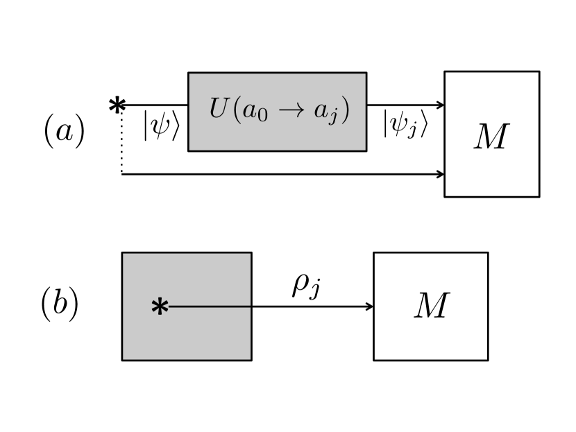
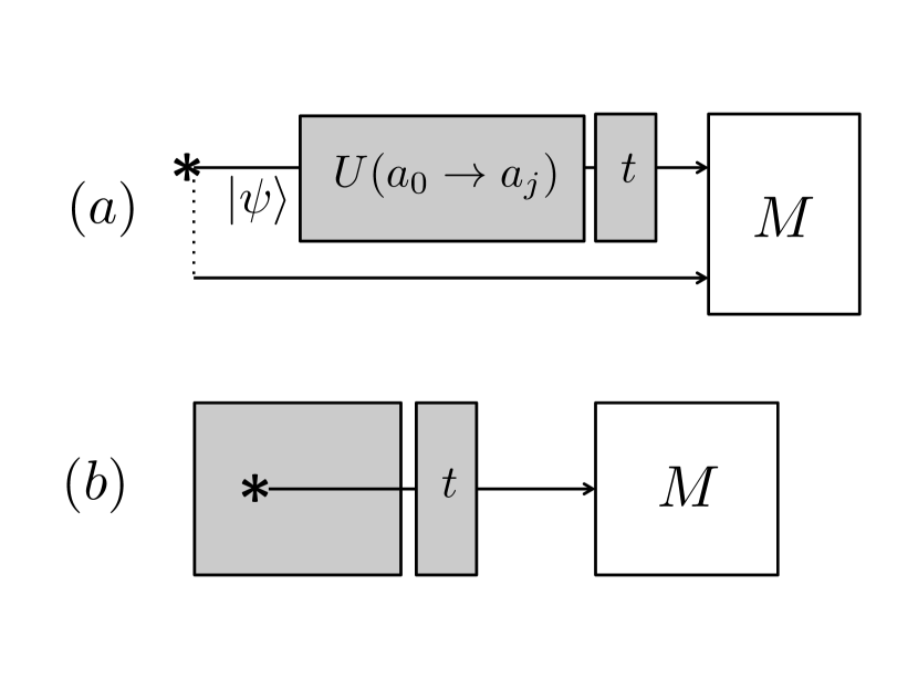
Mode discrimination takes different forms, depending on the experimental scenario that is considered. We shall consider two scenarios in this paper. The channel-discrimination scenario [Figure 1 (a)], the mode is created by the unitary channel that maps a default mode onto one of the . The source of light is in the hands of the verifiers, who can therefore avail themselves of a reference beam (“idler”) in addition to the beam that will be sent through the channel (“signal”). Then, the phase of the mode signal relative to the idler is defined: for instance it becomes possible to discriminate from . If the reference is classical (i.e. an intense coherent state), as we shall assume here, the phase can be perfectly defined and the state in the channel can be taken to be pure; this choice is optimal for discrimination. The channel-discrimination scenario has a clearly metrological flavor: besides the obvious case of phase discrimination Demkowicz-Dobrzanski et al. (2009); Nair et al. (2012), it can be seen as a special case of quantum reading Pirandola (2011); Nair (2011); Bisio et al. (2011); Dall’Arno et al. (2012), in which the devices to be discriminated are the unitary channels mentioned above. We refer to Ref. Pirandola et al. (2018) for a review of such metrological schemes.
The situation is different in the source-discrimination scenario, in which the source of light is inside the same black box that performs the encoding of the mode, as sketched in panel (b) of Figure 1. From the point of view of the verifier, the phase of the signal mode is global and thus inaccessible. The state as seen from the verifier is the mixture over all possible values of the mode’s phase, which is diagonal in the Fock basis Mølmer (1997) 111This statement should not be misread as contradicting the known facts that successive pulses in a laser may have relative coherence Van Enk and Fuchs (2002), and that such coherence may affect the unconditional security of cryptographic protocols, even if the encoding of classical information ignores those phases Lo and Preskill (2007). For one, here the modes to be discriminated may include relative phases between physical “pulses” (see e.g. Section IV.4). Once these modes are decided, we are studying single-shot discrimination, a task for which possible phases between successive instances of the modes indeed will not matter. In other words, we do not need to request the source to perform active phase randomization, for the state to be Fock-diagonal.. The flavor of the source-discrimination scenario is more cryptographic. Information is encoded in the modes in all the discrete-variable (e.g. BB84 Bennett and Brassard (1984)) and distributed-phase-reference (e.g. DPS Inoue et al. (2002), COW Stucki et al. (2005)) protocols for quantum key distribution (QKD); and also in protocols other than QKD, for instance quantum fingerprinting Arrazola and Lütkenhaus (2014); Jachura et al. (2017). For all these protocols, Eve ultimately wants to learn the mode in which the signals were encoded. Of course, the analysis of a cryptographic protocol goes beyond single-shot mode discrimination Scarani et al. (2009); Xu et al. (2020); Pirandola et al. (2020). This may be the reason why, to the best of our knowledge, the latter has not been previously studied in the source-discrimination scenario.
In this paper, we provide recipes to compute upper bounds for single-shot discrimination (both probabilistic and unambiguous) of any set of modes i.e. for arbitrary commutation relations (1). Specifically, we show that those optimizations can be cast a semidefinite programming (SDP) relaxation based on the work of Ref. Wang et al. (2019). We present the recipes for the channel-discrimination scenario in Section II, and that for the source-discrimination scenario in Section III. In Section IV we illustrate our method with several case studies: two modes (IV.1), phase discrimination (IV.2), a family of modes and its Fourier-dual family (IV.3), and the modes that appear in the DPS QKD protocol (IV.4). Finally, in Section V we discuss the extension of our study when losses are present between the device that encodes the modes and the measurement.
II Channel-discrimination scenario
Let us first consider the channel-discrimination scenario. Suppose there are different optical modes , with commutation relations given by Eq. (1). As mentioned previously, in the presence of reference beam, the phase of the signal mode could be defined relative to the the phase of the reference beam. Hence, the receiver’s task is to discriminate between pure states where
| (2) |
where is an arbitrary complex number such that is the probability of the source emitting photons. We also introduced the shorthand denoting the -photon state in the mode . The inner-product of the states associated to different modes can be computed easily
| (3) |
Note that the inner-product depends only on the photon number distribution and the commutation relations between different mode defined in Eq. (1).
II.1 Probabilistic mode discrimination
We first consider the setting for probabilistic discrimination. For uniform priors (our method can be easily generalised to any fixed priors), the optimal guessing probability is given by
| (4) |
where is the POVM element associated with the outcome and is the coefficient of the state when written in the photon number basis. In other words, we have to optimize both the state and the measurements that maximize the guessing probability, subject to the energy constraint. Let us now cast this optimization into a SDP by adapting the techniques of Wang et al. (2019). Before getting to it, we notice that Wang et al. (2019); Navascués et al. (2007, 2008) considers a hierarchy of semidefinite relaxations, which in general only yield upper bounds on the guessing probability. However, since we only consider a single receiver with no classical inputs, going into the second level of the hierarchy will satisfy the rank loop condition Navascués et al. (2008) and hence the first level of the hierarchy is actually tight.
Here comes the construction. Consider the set . As discussed in Wang et al. (2019); Navascués et al. (2007, 2008), the can be taken as projective measurements without any loss of generality. Denoting the elements of , one can define a set of vectors . Since all Gram matrices are positive semidefinite (PSD), so is the Gram matrix associated to the set . Hence we have
| (5) |
where the last relation is Eq. (3) and determines the entries of associated with .
However, this is an optimization problem with infinitely many variables and hence is computationally intractable. We then relax it by truncating the number of photons to (i.e. we’ll have variables ). We do it in such a way as to obtain an upper bound on the mode discrimination probabilities: that is, we derive some necessary (but not sufficient) conditions on the photon number distribution, and as a result the feasible region may be larger than the one allowed by quantum theory. Clearly, the relaxation can be made arbitrarily tight by increasing the photon number cut-off; and we expect when .
We then define the truncated state
| (6) |
that is sub-normalised:
| (7) |
The inner-product of the truncated states is
| (8) |
and its difference with the inner product of the full states can be bounded as
| (9) |
where the first inequality is a consequence of triangle inequality and the second inequality is due to the fact that . The constraint on the mean photon number can be relaxed to
| (10) |
All in all, we have with
| (11) |
where the last constraint uses the expressions (8) and (9). That constraint is linear in the when is real; when is complex, we can re-write it as
| (12) |
which is a matrix inequality linear in the , hence a valid SDP constraint.
II.2 Unambiguous mode discrimination
The same technique can be adapted to find the maximum success probability for unambiguous mode discrimination. For unambiguous discrimination, one must allow for the inconclusive outcome, which we associate to the POVM element . The Gram matrix will correspondingly increase in size to . Then we must add the constraint that the probability of error is zero
| (13) |
In the study of unambiguous discrimination, the aim is to minimize the probability of the inconclusive outcome or, equivalently, to maximize the success probability. Assuming uniform priors, the success probability is given by
| (14) |
Note that both the success probability and the error probability are linear functions of the Gram matrix . Hence, putting everything together, we have with
| (15) |
Recall that unambiguous state discrimination is possible if and only if the states to be discriminated are linearly independent. But unambiguous mode discrimination is possible even for linearly dependent modes, as the linear independence of the states is provided by the multiphoton components. In fact, the families studied in subsections IV.2, IV.3 and IV.4 will be linearly dependent.
III Source-discrimination scenario
In the source-discrimination scenario, the task is to discriminate between states that are diagonal in the Fock basis, subject to the energy constraint. Indeed, even assuming that the source produces a pure state
| (16) |
(this is Eq. (2) with explicit mention of the global phase of the signal mode), in the absence of a reference beam, the information available to the receiver is the phase-randomized state
| (17) |
Since the states to be discriminated are diagonal in the Fock basis, nothing is lost if the receiver starts by measuring the number of photons, then uses the best discrimination strategy for the given value of . This will manifest itself in the possibility of splitting the optimization in two steps.
III.1 Probabilistic mode discrimination
For probabilistic mode discrimination, the guessing probability is given by
| (18) |
where
| (19) |
is the optimal guessing probability for photons. Therefore, as expected, we can split the optimization into two steps. In the first step, we solve (19) for each value of . This can be done using the SDP technique of Ref. Wang et al. (2019). Similar to what we have done in the channel-discrimination scenario, consider the set which are Fock state from the set of modes . We define the set of vectors . Now, denote the Gram matrix associated to by . The SDP to bound is
| (20) |
which we have to solve for each photon number . In the second step, having for each photon number , we just need to enforce the energy constraint. This remaining step is linear programming (LP):
| (21) |
Like in the channel-discrimination scenario, we have infinitely many variables , so we need a cutoff that relaxes the original LP. With the same arguments as above, the resulting relaxation is given by
| (22) |
Notice that this relaxation is equivalent to assuming that the modes are perfectly distinguishable for . This is a good approximation when we pick sufficiently high photon number cutoff .
III.2 Unambiguous mode discrimination
Also for unambiguous state discrimination the optimal success probability is of the form
| (23) |
and can be bounded in two steps. In the first step, is computed from the SDP
| (24) |
where the last constraint captures the unambiguous discrimination condition
| (25) |
which is indeed satisfied if and only if for all whenever , . In the second step, the energy constraint is enforced in a LP, which we write down directly for the relaxation with a photon-number cutoff:
| (26) |
III.3 Towards an analytical solution of the LP
We have just seen that the final step of the optimization for the source-discrimination scenario is a LP of the form
| (27) |
where for probabilistic discrimination and for unambiguous discrimination. For a given , this LP can be solved analytically. We are going to show how this can be done, and highlight a condition on under which the solution can be easily spelled out.
The LP (27) is written in the so-called primal form. One could also consider its dual form given by Boyd and Vandenberghe (2004)
| (28) |
Due to the strong duality of LP, we know that and hence it is sufficient to solve the dual problem.
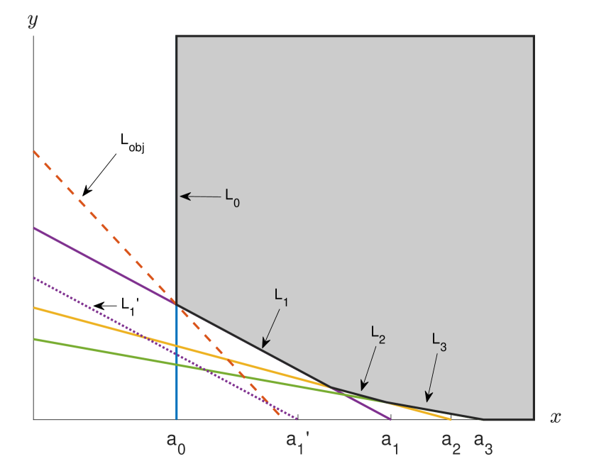
Whereas the primal problem is an optimization over infinitely many variables with a few equality constraints, the dual problem is an optimization over two variables with infinitely many constraints, which define the feasible region. The way to solve the dual problem is easily understood geometrically (Fig. 2). One traslates the lines with fixed gradient , till finding the lowest one that has at least one point in the feasible region. But the boundary of the feasible region is given by segments of straight lines of gradient . So the limiting line may touch the boundary of the feasible set either in a single point (the intersection of two , as illustrated in the figure) or in a whole segment. The latter can only happen if , but this is not the only condition: it is further necessary that contributes to the boundary of the feasible region. This may not always be the case, as illustrated in Fig. 2. By this recipe, one can always find the solution, given the .
It is worth describing in detail the case where all the constraints in (28), i.e. all the , contribute to the boundary of the feasible region in a non-trivial way. Given that the gradient of is , a necessary and sufficient condition for the boundary to be as described is that where are the coordinates of the intersection of with . From one immediately finds . Thus, will be the case if and only if
| (29) |
If this condition is satisfied, then the optimal discrimination takes up a very clear form. Indeed, for a boundary as described:
-
(i)
If , the intersection that defines will be with a single point, namely the intersection of and . The optimal state is then a mixture of two Fock states with these numbers, and the suitable weights.
-
(ii)
If , the intersection that defines will be the whole segment of gradient , and the optimal state with be the Fock state .
In other words, the solution of the LP will be , with
| (30) |
Thus, in many cases we can expect the optimal state for discrimination to consist of the Fock state if , and of the suitable mixture of the Fock states and if . However, condition (29) does not always hold: in subsection IV.3 we shall see an example where it is not met for , and indeed the Fock state will not be optimal for .
IV Case studies
We have derived efficient relaxations for estimating the parameters of mode discrimination, both probabilistic and unambiguous, in both the channel-discrimination and the source-discrimination scenario. In this Section, we discuss some case studies.
IV.1 Two modes
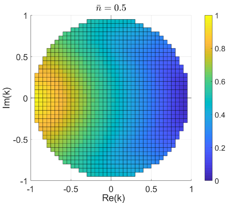
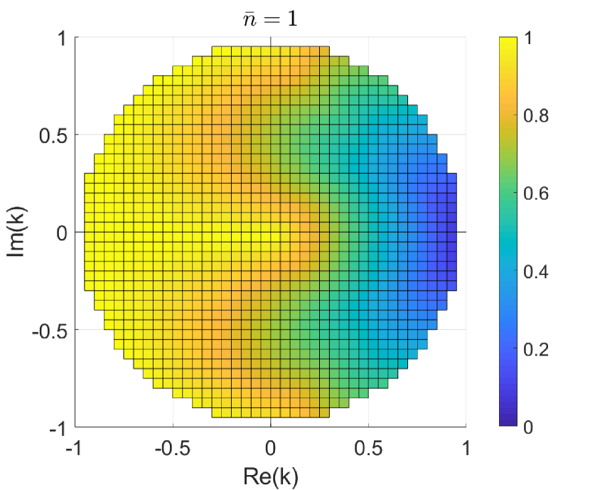
The discrimination between two modes is determined by a single parameter
| (31) |
When , the two modes are identical and therefore indistinguishable. When , the two modes are orthogonal and can be perfectly distinguished when .
Besides using our numerical tools, we are going to derive analytical solutions, exploiting the fact that the discrimination of two equally probable pure states has been solved long ago for both probabilistic Helstrom (1969) and unambiguous discrimination Ivanovic (1987); Dieks (1988); Peres (1988):
| (32) |
With this, single-shot discrimination of two modes in the source-discrimination scenario can be fully solved analytically. Indeed, there is no need to solve the SDPs (20) and (24) since we know from (32) that and (notice that everything depends on .). Moving to the LP, it is immediate to verify that both expressions satisfy condition (29). So we can import from subsection III.3 that the solution is
| (33) |
with the given in (30).
In the channel-discrimination scenario, we know from (32) that and with
| (34) |
where we used the expression (3) of the scalar product. Instead of the SDPs, we could try and solve (34).
For , it is a LP of the form (28) with (notice that here we are minimizing, whence the sign). Condition (29) reads and is therefore satisfied: so we know that the solution is
| (35) |
with the given in (30). The corresponding optimal state is for any . This value of shows that is larger than in the source-discrimination scenario (33), since ; while the value of is identical in the two scenarios.
For , the optimization (34) is also LP; but whether the absolute value adds a minus sign or not (i.e. whether or ) is not known a priori. One would therefore have to solve the two LPs, then compare the solutions. In either case, condition (29) would be satisfied only for alternate , and so the solution is not expected to involve only and . As for , the optimization (34) is quadratic, and there is no guarantee that an analytical solution can be found.
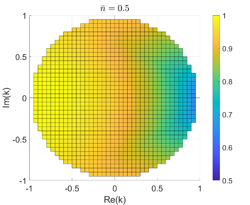
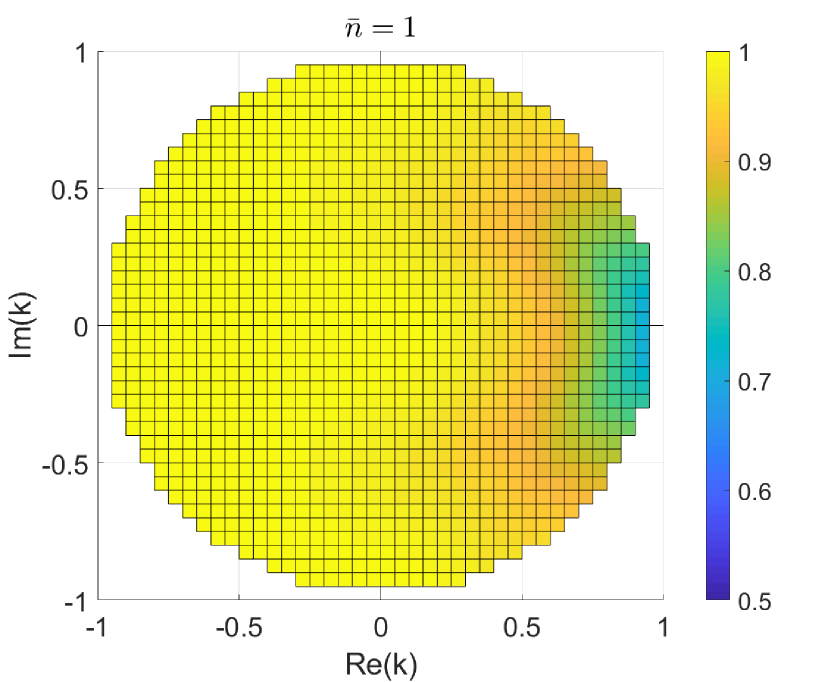
We thus turn to our SDPs (11) and (15). The results are shown in Fig. 3 for probabilistic discrimination, and in Fig. 4 for unambiguous discrimination. As expected, the modes are harder to distinguish when . More remarkable is the fact that distinguishability improves significantly in the region of negative phases. For instance, while it is known and rather obvious that perfect discrimination for becomes possible for , we see that when the modes can already be perfectly distinguished for (more in Section IV.2).
IV.2 Phase discrimination
Next we consider the problem of phase discrimination. Since the phase of an optical mode is not defined unless a reference beam is provided, this case study is restricted to the channel-discrimination scenario. The receiver’s task is to guess one of a set of unitary channels where is the number operator in the signal mode. In other words, the receiver can use pure states to distinguish modes of the form
| (36) |
where is the initial signal mode prior to the phase-shift.
Our formalism can be applied to any set of phases to be discriminated. For the numerical case study, we choose the symmetric set , whose probabilistic discrimination has been studied in the context of quantum sensing Nair et al. (2012). The commutation relations are then given by
| (37) |
For probabilistic discrimination (see Fig. 5(a)), our SDP (11) recovers the same bound as Theorem 3 of Ref. Nair et al. (2012). The study of unambiguous discrimination is novel: the result is plotted in Fig. 5(b). Also notice that, for , the modes in this family are linearly dependent; but, as discussed, unambiguous discrimination is possible because one can create linearly independent states.
The case corresponds to in Section IV.1. As we notice there and see again here, perfect discrimination becomes possible at . This is because the pure states with are orthogonal. Indeed, , while . Since distinguishability cannot decrease when increasing , one expects to find two orthogonal states for any . Indeed, these are with and . In general these are superpositions of three Fock states, reducing to two only when (). Thus, as anticipated, the optimal state does not obey (30).
IV.3 Computational and Fourier transform basis modes
As our next example, we consider a family made of two sets of orthogonal modes. The first set are called computational basis modes. The second set are called Fourier transform basis modes and are defined as
| (38) |
where is the -th root of unity. This family of modes have appeared in quantum cryptography: the classical information is encoded into these modes in the famous BB84 protocol Bennett and Brassard (1984) for , and the case defines one of its possible generalizations to higher alphabets Sheridan and Scarani (2010). However, in those QKD protocols the classical information is encoded in the mode’s index: one wants to determine , whether from or . By contrast, here we stay with the task of mode discrimination, and study both probabilistic and unambiguous discrimination from the set .
For given , the commutation relations are
| (39) |
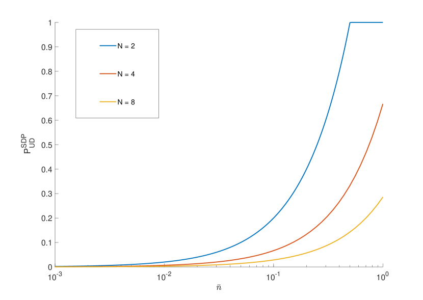
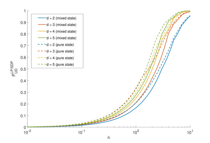
We set and solve the SDP and/or LP for varying from to 10, and for . The results for probabilistic discrimination are shown in Fig. 6(a); those for unambiguous discrimination in 6(b); both figures contain information about the channel-discrimination scenario (dashed) and the source-discrimination scenario (solid).
Channel discrimination is more powerful than source discrimination: while more marked for probabilistic discrimination, the difference is also present in unambiguous discrimination, contrary to what was the case for two modes (Section IV.1). Another feature present in both figures, again more marked for probabilistic discrimination, is a crossover of behavior as a function of : for , the discrimination is better for smaller ; whereas for , the discrimination is better for higher . This can be understood qualitatively. In the limit , guessing the mode is hardly more than a random pick from a uniform distribution, so the guessing probability is close to and decreases with . In the limit of large , decreases with and therefore the distinguishability increases.
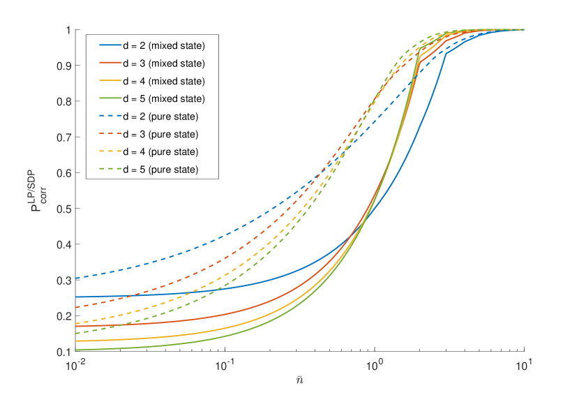
In the source-discrimination scenario, we find that condition (29) is generally not satisfied for , either for probabilistic or unambiguous discrimination.
For unambiguous discrimination, the reason is clear: the single-photon states are linearly dependent and hence unambiguous discrimination is not possible. In order for unambiguous discrimination to be possible, the state must contain some multi-photon component.
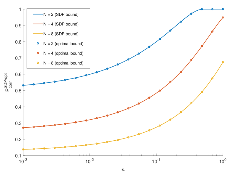
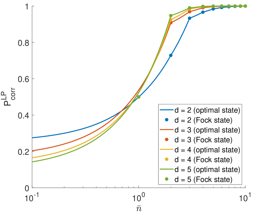
For probabilistic discrimination, we find that the condition (29) is violated for . To see that, we compare with that of Fock states in Fig. 7. For , the single-photon bound is . This corresponds to a simple strategy: betting on one of the bases and measure in it.
IV.4 Differential-phase-shift modes
Lastly, we consider a family of modes inspired by the differential-phase-shift (DPS) QKD protocol Inoue et al. (2002). In the protocol, the information is encoded in the relative phase between subsequent temporal modes. Abstractly, to any -bit strings , a mode is associated according to
| (40) |
where the are orthogonal modes (temporal ones in the original setting) and where
| (41) |
with the -th bit of the string (by convention, we set the phase of the reference mode for all ). For a given , there are different modes, only linearly-many of which are orthogonal among the ones. The commutation relation for the modes associated to string and can be computed recursively using the relation (41) and is given by
| (42) |
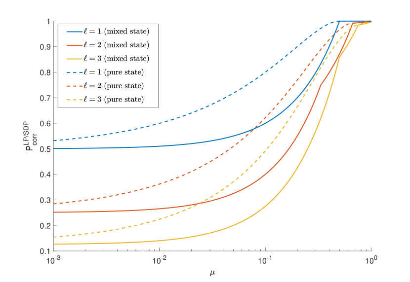
Since the SDP scales badly with , in this paper we present the results only for . When , the two modes to be distinguished are orthogonal, and so this is a special case of what we studied in Section IV.1. For , the four modes are all non-orthogonal. The eight modes for form two sets of four orthogonal modes.
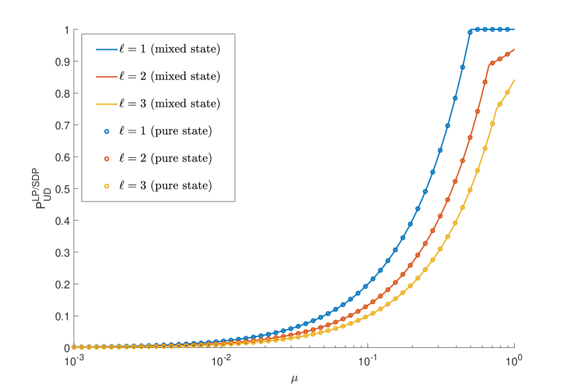
The results of our numerical method are shown in Fig. 8(a) for probabilistic discrimination, and in Fig. 8(b) for unambiguous discrimination. Since the family given by is constructed from orthogonal modes (“pulses”), we found it more appropriate to compare the families for a given value of the energy per pulse , rather than of the total energy . Even with this scaling, it proves more difficult to distinguish within a set with higher , since the receiver has to discriminate more modes.
Comparing the mixed state encoding to the pure state encoding, we find that the pure state encoding is more distinguishable only in the probabilistic discrimination setting. Remarkably, we find that the mixed state bounds coincide with that of the pure state encoding for the unambiguous discrimination setting.
V Coda: on losses
In this last Section, we review how the ultimate limits of mode discrimination are modified when there are mode-independent losses between the device to be tested and the measurement, as sketched in Fig. 9. This is modelled as a beam splitter transformation where and can be taken as real and positive and . The state that arrives at the measurement station is now the partial state associated with the transmitted output.
The study of the source-discrimination scenario remains practically unchanged. Indeed, losses do not introduce any coherence between photon number states. So, if the state before the losses is given by Eq. (17), the state after the losses will still be a number mixture with
| (43) |
If still represents the energy constraint for the input state, one solves the LP under the energy constraints to get the . The to be prepared are then obtained by inverting the linear system of equations (43). The only practical worries may come from numerical cutoffs in this inversion when is large.
On the contrary, the optimizations in the channel-discrimination scenario can no longer be cast as SDPs. Indeed, the initially pure state becomes mixed with losses. Thus, on the one hand, we cannot build Gram matrices as we did in Section II. But on the other hand, the basis in which the mixed state is diagonal is not fixed, and is definitely not the Fock basis: so we cannot adapt the approach of Section III either.
In some simple cases, a heuristic optimization may still be trustful. For instance, let us look at the probabilistic discrimination of two modes with . We know Helstrom (1969) that the probability of discriminating correctly between two equally probable mixed states is given by . One can then write the algorithm that, given a in the form (2), computes the obtained after losses; then heuristically maximizes the trace distance over the complex parameters under the energy constraint for the initial states. We implemented this procedure using the function fmincon of MATLAB. Inspection of the numerical solutions we obtained indicates that the relevant parameter in the input state are the , while the arguments of the (relative phases) do not seem to matter, just as in the lossless case (34).
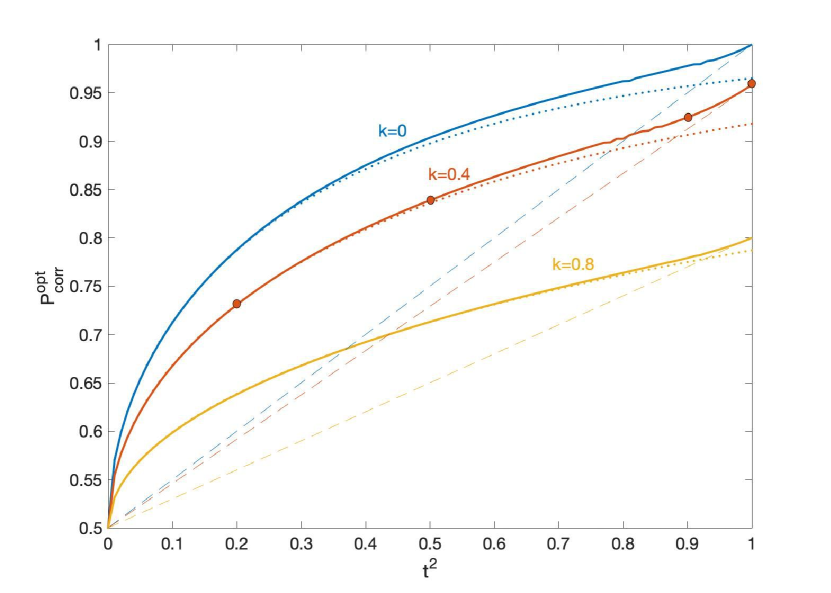
An example is given in Fig. 10. The constraint is set at : thus, in the absence of losses, the optimal state is the Fock state . When losses increase, this state becomes quickly sub-optimal, while the probability of guessing correctly approaches the value corresponding to choosing a coherent state as input state (see also Table 1). Based on this observation, whenever integer, for the sake of estimates one could use
| (44) |
because the two probabilities on the r.h.s. can be given analytically. Indeed, on a beam-splitter, a coherent state splits as ; so the states in the transmitted mode are pure, and a standard calculation gives , and finally . For a -photon Fock state, the transmitted state reads with . Because it’s diagonal in the number basis, the optimal measurement to discriminate between the modes can be seen as: first, measure the photon number and thus project in a Fock state; then distinguish between the two Fock states. Thus .
| 1 (Fock) | 0 | 1 | 0 | 0 | 0 | 0 |
|---|---|---|---|---|---|---|
| 0.9 | 0.1458 | 0.7088 | 0.1454 | 0.0000 | 0.0000 | 0.0000 |
| 0.5 | 0.3075 | 0.4363 | 0.2092 | 0.0430 | 0.0039 | 0.0001 |
| 0.2 | 0.3450 | 0.3914 | 0.1952 | 0.0567 | 0.0105 | 0.0012 |
| coh | 0.3679 | 0.3679 | 0.1839 | 0.0613 | 0.0153 | 0.0031 |
VI Conclusion
In this paper, we have presented efficient methods to compute the ultimate limits for single-shot discrimination of optical modes. The methods, based on linear and semi-definite programming, apply to any set of modes with any prior distribution (we wrote the paper for the uniform prior not to introduce further notation, but the modifications are obvious). The bounds that are obtained can be used as fundamental benchmark for the performance of realistic devices or measurement schemes.
We pointed out the importance of stating whether the verifier has the possibility of defining a reference frame for the modes’ phase. Depending on the family of modes that is considered, the difference in discrimination is found to be significant; and of course, some tasks like phase discrimination make only sense if the reference is available. Note that we assumed that one the reference beam is classical and hence its phase relative to the receiver’s reference frame could be determined with arbitrary precision. We leave the study of the channel-discrimination scenario with a weak reference beam as an open problem.
Let us finish by pointing out two related topics that we have not dealt with in the current work. First: throughout the paper, the characterization of the optical modes has been taken as known and perfect. It is known that this could be relaxed in some situations. Indeed, randomness of quantum origin can be certified from the measurement of uncharacterized optical modes, based only on an energy constraint Van Himbeeck et al. (2017). Second: we have considered single-shot discrimination. For the discrimination of unitaries, it is known that perfect discrimination is always possible if one has enough many copies Acín (2001), and a similar result for energy-constrained discrimination has been described recently Becker et al. (2020).
Acknowledgments
We thank Chee Wei Soh for help in the first part of this project, and Konrad Banaszek, Alessandro Bisio, Michele Dall’Arno, Claude Fabre, Charles Lim, Norbert Lütkenhaus, Matteo Paris and Stefano Pirandola for comments and suggestions. This research is supported by the National Research Foundation and the Ministry of Education, Singapore, under the Research Centres of Excellence programme.
References
- Fabre and Treps (2019) C. Fabre and N. Treps, “Modes and states in quantum optics,” (2019), preprint arXiv:1912.09321.
- Demkowicz-Dobrzanski et al. (2009) R. Demkowicz-Dobrzanski, U. Dorner, B. J. Smith, J. S. Lundeen, W. Wasilewski, K. Banaszek, and I. A. Walmsley, Phys. Rev. A 80, 013825 (2009).
- Nair et al. (2012) R. Nair, B. J. Yen, S. Guha, J. H. Shapiro, and S. Pirandola, Phys. Rev. A 86, 022306 (2012).
- Pirandola (2011) S. Pirandola, Phys. Rev. Lett. 106, 090504 (2011).
- Nair (2011) R. Nair, Phys. Rev. A 84, 032312 (2011).
- Bisio et al. (2011) A. Bisio, M. Dall’Arno, and G. M. D’Ariano, Phys. Rev. A 84, 012310 (2011).
- Dall’Arno et al. (2012) M. Dall’Arno, A. Bisio, G. M. D’Ariano, M. Miková, M. Ježek, and M. Dušek, Phys. Rev. A 85, 012308 (2012).
- Pirandola et al. (2018) S. Pirandola, B. R. Bardhan, T. Gehring, C. Weedbrook, and S. Lloyd, Nature Photonics 12, 724 (2018).
- Mølmer (1997) K. Mølmer, Phys. Rev. A 55, 3195 (1997).
- Note (1) This statement should not be misread as contradicting the known facts that successive pulses in a laser may have relative coherence Van Enk and Fuchs (2002), and that such coherence may affect the unconditional security of cryptographic protocols, even if the encoding of classical information ignores those phases Lo and Preskill (2007). For one, here the modes to be discriminated may include relative phases between physical “pulses” (see e.g. Section IV.4). Once these modes are decided, we are studying single-shot discrimination, a task for which possible phases between successive instances of the modes indeed won’t matter. In other words, we don’t need to request the source to perform active phase randomization, for the state to be Fock-diagonal.
- Bennett and Brassard (1984) C. H. Bennett and G. Brassard, in Proc. of IEEE Int. Conf. on Comp., Syst. and Signal Proc., Bangalore, India, Dec. 10-12, 1984 (1984).
- Inoue et al. (2002) K. Inoue, E. Waks, and Y. Yamamoto, Physical review letters 89, 037902 (2002).
- Stucki et al. (2005) D. Stucki, N. Brunner, N. Gisin, V. Scarani, and H. Zbinden, Applied Physics Letters 87, 194108 (2005).
- Arrazola and Lütkenhaus (2014) J. M. Arrazola and N. Lütkenhaus, Phys. Rev. A 89, 062305 (2014).
- Jachura et al. (2017) M. Jachura, M. Lipka, M. Jarzyna, and K. Banaszek, Opt. Express 25, 27475 (2017).
- Scarani et al. (2009) V. Scarani, H. Bechmann-Pasquinucci, N. J. Cerf, M. Dušek, N. Lütkenhaus, and M. Peev, Rev. Mod. Phys. 81, 1301 (2009).
- Xu et al. (2020) F. Xu, X. Ma, Q. Zhang, H.-K. Lo, and J.-W. Pan, Reviews of Modern Physics 92, 025002 (2020).
- Pirandola et al. (2020) S. Pirandola, U. L. Andersen, L. Banchi, M. Berta, D. Bunandar, R. Colbeck, D. Englund, T. Gehring, C. Lupo, C. Ottaviani, J. L. Pereira, M. Razavi, J. S. Shaari, M. Tomamichel, V. C. Usenko, G. Vallone, P. Villoresi, and P. Wallden, Adv. Opt. Photon. 12, 1012 (2020).
- Wang et al. (2019) Y. Wang, I. W. Primaatmaja, E. Lavie, A. Varvitsiotis, and C. C. W. Lim, npj Quantum Information 5, 1 (2019).
- Navascués et al. (2007) M. Navascués, S. Pironio, and A. Acín, Physical Review Letters 98, 010401 (2007).
- Navascués et al. (2008) M. Navascués, S. Pironio, and A. Acín, New Journal of Physics 10, 073013 (2008).
- Boyd and Vandenberghe (2004) S. P. Boyd and L. Vandenberghe, Convex optimization (Cambridge university press, 2004).
- Helstrom (1969) C. W. Helstrom, Journal of Statistical Physics 1, 231 (1969).
- Ivanovic (1987) I. Ivanovic, Physics Letters A 123, 257 (1987).
- Dieks (1988) D. Dieks, Physics Letters A 126, 303 (1988).
- Peres (1988) A. Peres, Physics Letters A 128, 19 (1988).
- Sheridan and Scarani (2010) L. Sheridan and V. Scarani, Physical Review A 82, 030301 (2010).
- Van Himbeeck et al. (2017) T. Van Himbeeck, E. Woodhead, N. J. Cerf, R. García-Patrón, and s. Pironio, Quantum 1, 33 (2017).
- Acín (2001) A. Acín, Phys. Rev. Lett. 87, 177901 (2001).
- Becker et al. (2020) S. Becker, N. Datta, L. Lami, and C. Rouzé, “Energy-constrained discrimination of unitaries, quantum speed limits and a gaussian solovay-kitaev theorem,” (2020), preprint arXiv:2006.06659.
- Van Enk and Fuchs (2002) S. J. Van Enk and C. A. Fuchs, Quant. Inf. Comput. 2, 151 (2002).
- Lo and Preskill (2007) H.-K. Lo and J. Preskill, Quant. Inf. Comput. 7, 431 (2007).