Optimal Strategies for Graph-Structured Bandits

1 Introduction

The multi-armed bandit problem is a popular framework to formalize sequential decision making problems. It was first introduced in the context of medical trials (Thompson, 1933, 1935) and later formalized by Robbins (1952). In this paper, we consider a contextual and structured variant of the problem, specified by a set of distributions $\nu\!=\!(\nu_{a,b})_{a\in\mathcal{A},b\in\mathcal{B}}$ with means $(\mu_{a,b})_{a\in\mathcal{A},b\in\mathcal{B}}$ , where $\mathcal{A}$ is a finite set of arms and $\mathcal{B}$ is a finite set of users. Such $\nu$ is called a (bandit) configuration where each $\nu_{b}\!=\!(\nu_{a,b})_{a\in\mathcal{A}}$ can be seen as a classical multi-armed bandit problem. The streaming protocol is the following: at each time $t\!\geqslant\!1$ , the learner deals with a user $b_{t}\!\in\!\mathcal{B}$ and chooses an arm $a_{t}\!\in\!\mathcal{A}$ , based only on the past. We consider two scenarios: either the sequence of users is deterministic (uncontrolled scenario) or the learner has the possibility to choose the user (controlled scenario), see Section 1.1. The learner then receives and observes a reward $X_{t}$ sampled according to $\nu_{a_{t},b_{t}}$ conditionally independent from the past. We assume binary rewards: each $\nu_{a,b}$ is a Bernoulli distribution $\textnormal{Bern}(\mu_{a,b})$ with mean $\mu_{a,b}\!\in\!(0,1)$ and we denote by $\mathcal{D}$ the set of such configurations. The goal of the learner is then to maximize its expected cumulative reward over $T$ rounds, or equivalently minimize regret given by

R(\nu,T)=\mathbb{E}_{\nu}\!\left[\sum\limits_{t=1}^{T}\max\limits_{a\in\mathcal{A}}\mu_{a,b_{t}}-X_{t}\right]\,.

For this problem one can run, for example, a separate instance of a bandit algorithm for each user $b$ , but we would like to exploit a known structure among the users (which we detail below).

Unstructured bandits

The classical bandit problem (when $|\mathcal{B}|\!=\!1$ ) received increased attention in the middle of the $20^{\text{th}}$ century. The seminal paper Lai and Robbins (1985) established the first lower bounds on the cumulative regret, showing that designing a strategy that is optimal uniformly over a given set of configurations $\mathcal{D}$ comes with a price. The study of the lower performance bounds in multi-armed bandits successfully lead to the development of asymptotically optimal strategies for specific configuration sets, such as the KL-UCB strategy (Lai, 1987; Cappé et al., 2013; Maillard, 2018) for exponential families, or alternatively the DMED and IMED strategies from Honda and Takemura (2011, 2015). The lower bounds from Lai and Robbins (1985), later extended by Burnetas and Katehakis (1997) did not cover all possible configurations, and in particular structured configuration sets were not handled until Agrawal et al. (1989) and then Graves and Lai (1997) established generic lower bounds. Here, structure refers to the fact that pulling an arm may reveal information that enables to refine estimation of other arms. Unfortunately, designing efficient strategies that are provably optimal remains a challenge for many structures at the cost of a high computational complexity.

Structured configurations

Motivated by the growing popularity of bandits in a number of industrial and societal application domains, the study of structured configuration sets has received increasing attention over the last few years: The linear bandit problem is one typical illustration (Abbasi-Yadkori et al., 2011; Srinivas et al., 2010; Durand et al., 2017), for which the linear structure considerably modifies the achievable lower bound, see Lattimore and Szepesvari (2017). The study of a unimodal structure naturally appears in the context of wireless communications, and has been considered in Combes and Proutiere (2014) from a bandit perspective, providing an explicit lower bound together with a strategy exploiting this structure. Other structures include Lipschitz bandits (Magureanu et al., 2014), and we refer to the manuscript Magureanu (2018) for other examples, such as cascading bandits that are useful in the context of recommender systems. Combes et al. (2017) introduced a generic strategy called OSSB (Optimal Structured Stochastic Bandit), stepping the path towards generic multi-armed bandit strategies that are adaptive to a given structure.

Graph-structure

In this paper, we consider the following structure: For a given weight matrix $\omega\!=\!(\omega_{b,b^{\prime}})_{b,b^{\prime}\in\mathcal{B}}\in[0,1]^{\mathcal{B}\times\mathcal{B}}$ inducing a metric on $\mathcal{B}$ , we assume that for any two users $b,b^{\prime}\!\in\!\mathcal{B}$ , $\left|\left|\mu_{b}\!-\!\mu_{b^{\prime}}\right|\right|_{\infty}\!\coloneqq\!\max_{a\in\mathcal{A}}\left|\mu_{a,b}\!-\!\mu_{a,b^{\prime}}\right|\!\leqslant\!\omega_{b,b^{\prime}}$ . We see the matrix $\omega$ as an adjacency matrix of a fully connected weighted graph where each vertex represents a user and each weigh $\omega_{b,b^{\prime}}$ measures proximity between two users, hence we call this a “graph structure”. The motivation to study such a structure is two-fold. On the one hand, in view of paving the way to solving generic structured bandits, the graph structure yields nicely interpretable lower bounds that show how $\omega$ effectively modifies the achievable optimal regret and suggests a natural strategy, while being flexible enough to interpolate between a fully unstructured and a highly structured setup. On the other hand, multi-armed bandits have been extensively applied to recommender systems: In such systems it is natural to assume that users may not react arbitrarily differently from each other, but that two users that are "close" in some sense will also react similarly when presented with the same item (action). Now, the similarity between any two users may be loosely or accurately known (by studying for instance activities of users on various social networks and refining this knowledge once in a while): The weight matrix $\omega$ enables to summarize such imprecise knowledge. Indeed $\omega_{b,b^{\prime}}\!=\!0$ means that two users behave identically, while $\omega_{b,b^{\prime}}\!=\!1$ is not informative on the true similarity $\|\mu_{b}\!-\!\mu_{b^{\prime}}\|_{\infty}$ that can be anything from arbitrarily small to $1$ . Hence, studying this structure is both motivated by a theoretical challenge and more applied considerations. To our knowledge this is the first work on graph structure. Other structured problems such as Clustered bandits (Gentile et al., 2014), Latent bandits (Maillard and Mannor, 2014), or Spectral bandits (Valko et al., 2014) do not deal with this particular setting.

Goal

The primary goal of this paper is to build a provably optimal strategy for this flexible notion of structure. To do so, we derive lower bounds and use them to build intuition on how to handle structure, which enables us to establish a novel bandit strategy, that we prove to be optimal. Although specialized to this structure, the mechanisms leading to the strategy and introduced in the proof technique are novel and are of independent interest.

Outline and contributions

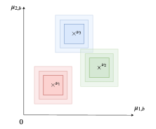
We formally introduce the graph-structure model in Section 1.2. Graph structure is simple enough while interpolating between a fully unstructured case and highly-structured settings such as clustered bandits (see Figure 1): This makes it a convenient setting to study structured multi-armed bandits. In Section 2, we first establish in Proposition 5 a lower bound on the asymptotic number of times a sub-optimal couple must be pulled by any consistent strategy (see Definition 3), together with its corresponding lower bound on the regret (see Corollary 8) involving an optimization problem. In Section 3, we revisit the Indexed Minimum Empirical Divergence (IMED) strategy from Honda and Takemura (2011) introduced for unstructured multi-armed bandits, and adapt it to the graph-structured setting, making use of the lower bounds of Section 2. The resulting strategy is called IMED-GS in the controlled scenario and IMED-GS₂ in the uncontrolled scenario. Our analysis reveals that in view of asymptotic optimality, these strategies may still not optimally exploit the graph-structure in order to trade-off information gathering and low regret. In order to address this difficulty, we introduce the modified IMED-GS^⋆ strategy for the controlled scenario (and IMED-GS ${}^{\star}_{2}$ in the uncontrolled one). We show in Theorem 11, which is the main result of this paper, that both IMED-GS^⋆ and IMED-GS ${}^{\star}_{2}$ are asymptotically optimal consistent strategies. Interestingly, IMED-GS^⋆ does not compute a solution to the optimization problem appearing in the lower bound at each time step, unlike for instance OSSB introduced for generic structures, but only about $\log(T)$ times after $T$ steps. Also, if forced exploration does not seem to be avoidable for this problem, IMED-GS^⋆ does not make use of an explicit forced exploration scheme but a more implicit one, based on local counters of empirical events. Up to our knowledge, IMED-GS^⋆ is the first strategy with such properties, in the context of a structure requiring to solve an optimization problem, that is provably asymptotically optimal. On a broader perspective, we believe the mechanism used in IMED-GS^⋆ as well as the proof techniques could be extended beyond the considered graph-structure, thus opening promising perspective in order to build structure-adaptive optimal strategies for generic structures. Last, we provide in Section 4 numerical illustrations on synthetic data. They show that IMED-GS^⋆ is also numerically efficient in practice, both in terms of regret minimization and computation time; this contrasts with some bandit strategies introduced for other structures (as in Combes et al. (2017), Lattimore and Szepesvari (2017)), that in practice suffer from a prohibitive burn-in phase.

1.1 Setting

Let us recall that the goal of the learner is to maximize its expected cumulative reward over $T$ rounds, or equivalently minimize regret given by

R(\nu,T)=\mathbb{E}_{\nu}\!\left[\sum\limits_{t=1}^{T}\max\limits_{a\in\mathcal{A}}\mu_{a,b_{t}}-X_{t}\right]\,.

As mentioned, for this problem one can run, for example, a separate instance of bandit algorithms for each user $b$ , but we would like to exploit the graph structure. We consider two typical scenarios.

Uncontrolled scenario

The sequence of users $(b_{t})_{t\geqslant 1}$ is assumed deterministic and does not depend on the strategy of the learner. At each time step $t\!\geqslant\!1$ , the user $b_{t}$ is revealed to the learner.

Controlled scenario

The sequence of users $(b_{t})_{t\geqslant 1}$ is strategy-dependent and at each time step $t\!\geqslant\!1$ , the learner has to choose a user $b_{t}$ to deal with, based only on the past.

Both scenarios are motivated by practical considerations: uncontrolled scenario is the most common setup for recommender systems, while controlled scenario is more natural in case the learner interacts actively with available users as in advertisement campaigns. In an uncontrolled scenario, the frequencies of user-arrivals are imposed and may be arbitrary, while in a controlled scenario all users are available and the learner has to deal with them with similar frequency (even if this means considering a subset of users). We formalize the notion of frequency in the following definition.

Definition 1 (Log-frequency of a user)

A sequence of user $(b_{t})_{t\geqslant 1}$ has log-frequencies $\beta\!\in\![0,1]^{\mathcal{B}}$ if, almost surely, the number of times the learner has dealt with user $b\!\in\!\mathcal{B}$ is $N_{b}(T)\!=\!\Theta\!\left(T^{\beta_{b}}\right)$ ¹¹1We say that $u_{T}=\Theta(v_{T})$ , if the two sequences $u_{T}$ and $v_{T}$ are equivalent.. In this case, almost surely we have

\forall b\in\mathcal{B},\ \lim\limits_{T\rightarrow\infty}\dfrac{\log\!\left(N_{b}(T)\right)}{\log(T)}=\beta_{b}\,.

In an uncontrolled scenario, we assume that the sequence of users $(b_{t})_{t\geqslant 1}$ has positive log-frequencies $\beta\!\in\!(0,1]^{\mathcal{B}}$ , with $\beta$ unknown to the learner. In a controlled scenario, we focus only on strategies that induce sequences of users with same log-frequencies, hence all equal to $1$ , independently on the considered configuration, that is strategies such that, almost surely, $N_{b}(T)\!=\!\Theta(T)$ for all user $b\!\in\!\mathcal{B}$ .

1.2 Graph Structure

In this section, we introduce the graph structure. We assume that all bandit configurations $\nu$ belong to a set of the form:

\overline{\mathcal{D}}_{\omega}\coloneqq\left\{\nu\in\mathcal{D}:\ \forall b,b^{\prime}\in\mathcal{B},\,\max\limits_{a\in\mathcal{A}}\left|\mu_{a,b}-\mu_{a,b^{\prime}}\right|\leqslant\omega_{b,b^{\prime}}\right\}\,,

where $\omega\!=\!(\omega_{b,b^{\prime}})_{b,b^{\prime}\in\mathcal{B}}\in[0,1]^{\mathcal{B}\times\mathcal{B}}$ is a weight matrix known to the learner. Intuitively, when the weights are close to $1$ , we expect no change to the agnostic situation. But, when the weights are close to $\|\mu_{b}\!-\!\mu_{b^{\prime}}\|_{\infty}\!\coloneqq\!\max_{a\in\mathcal{A}}\left|\mu_{a,b}\!-\!\mu_{a,b^{\prime}}\right|$ , we expect significantly lower achievable regret.

Remark 2

For the specific case where $\omega_{b,b^{\prime}}=0$ , $\overline{\mathcal{D}}_{\omega}$ corresponds to user $b$ and $b^{\prime}$ known to be perfectly clustered. The weight matrix given in Figure 1 models three smooth clusters of users. Each cluster is included in a ball of diameter $\alpha$ for the infinite norm $\|\cdot\|_{\infty}$ .

In the sequel we assume the following properties on the weights.

Assumption 1 (Metric weight property)

The weight matrix $\omega$ satisfies:

-

$\omega_{b,b}\!=\!0$ and $\omega_{b,b^{\prime}}\!>\!0$ for all $b\!\neq\!b^{\prime}\!\in\!\mathcal{B}$ ,
-

$\omega_{b,b^{\prime}}\!=\!\omega_{b^{\prime},b}$ and $\omega_{b,b^{\prime}}\!\leqslant\!\omega_{b,b^{\prime\prime}}\!+\!\omega_{b^{\prime\prime},b^{\prime}}$ for all $b,b^{\prime},b^{\prime\prime}\!\in\!\mathcal{B}$ .

This comes without loss of generality, since for the first property, if two users share exactly the same distribution we can see them as one unique user. For the second property, considering $\widetilde{\omega}_{b,b^{\prime}}\!=\!\sup_{a\in\mathcal{A},\nu\in\overline{\mathcal{D}}_{\omega}}{\left|\mu_{a,b}\!-\!\mu_{a,b^{\prime}}\right|}$ leads to the same set of configuration $\overline{\mathcal{D}}_{\omega}\!=\!\overline{\mathcal{D}}_{\widetilde{\omega}}$ and it holds $\widetilde{\omega}_{b,b^{\prime}}\!=\!\widetilde{\omega}_{b^{\prime},b}$ , $\widetilde{\omega}_{b,b^{\prime}}\!\leqslant\!\widetilde{\omega}_{b,b^{\prime\prime}}\!+\!\widetilde{\omega}_{b^{\prime\prime},b^{\prime}}$ . Such a weight matrix $\omega$ naturally induces a metric on $\mathcal{B}^{2}$ .

Refer to caption — Figure 1: A cluster structure. Left: weight matrix of three clusters. Right: range of two armed bandit problems included in clusters with center $(\nu_{1},\nu_{2},\nu_{3})$ for various $\alpha$ (the larger $\alpha$ the lighter and larger the box). The value $\alpha\!=\!0$ corresponds to perfect clusters.

1.3 Notations

Let $\mu_{b}^{\star}\!=\!\max_{a\in\mathcal{A}}{\mu_{a,b}}$ denote the optimal mean for user $b$ and $\mathcal{A}_{b}^{\star}\!=\!\mathop{\mathrm{argmax}}_{a\in\mathcal{A}}{\mu_{a,b}}$ the set of optimal arms for this user. We define for a couple $(a,b)\!\in\!\mathcal{A}\!\times\!\mathcal{B}$ its gap $\Delta_{a,b}\!=\!\mu^{\star}_{b}\!-\!\mu_{a,b}$ . Thus a couple is optimal if its gap is equal to zero and sub-optimal if it is positive. We denote by $\mathcal{O}^{\star}\!=\!\left\{(a,b)\!\in\!\mathcal{A}\!\times\!\mathcal{B}\!:\mu_{a,b}\!=\!\mu_{b}^{\star}\right\}$ the set of optimal couples. Thanks to the chain rule we can rewrite the regret as follows:

R(\nu,T)=\sum_{a,b\in\mathcal{A}\times\mathcal{B}}\Delta_{a,b}\,\mathbb{E}_{\nu}\big{[}N_{a,b}(T)\big{]}\,,\quad\text{where }N_{a,b}(t)=\sum_{s=1}^{t}\mathbb{I}_{\big{\{}(a_{s},b_{s})=(a,b)\big{\}}}

is the number of pulls of arm $a$ and user $b$ up to time $t$ .

2 Regret Lower bound

In this subsection, we establish lower bounds on the regret for the structure $\overline{\mathcal{D}}_{\omega}$ . In order to obtain non trivial lower bounds we consider, as in the classical bandit problem, strategies that are consistent (uniformly good) on $\overline{\mathcal{D}}_{\omega}$ .

Definition 3 (Consistent strategy)

A strategy is consistent on $\overline{\mathcal{D}}_{\omega}$ if for all configuration $\nu\!\in\!\overline{\mathcal{D}}_{\omega}$ , for all sub-optimal couple $(a,b)$ , for all $\alpha\!>\!0$ ,

\lim\limits_{T\rightarrow\infty}\mathbb{E}_{\nu}\!\left[\dfrac{N_{a,b}(T)}{N_{b}(T)^{\alpha}}\right]=0\,.

Remark 4

When $\mathcal{B}\!=\!\{b\}$ , $N_{b}(T)\!=\!T$ and we recover the usual notion of consistency (Lai and Robbins, 1985).

Before we provide below the lower bound on the cumulative regret, let us give some intuition: To that end, we fix a configuration $\nu\!\in\!\overline{\mathcal{D}}_{\omega}$ and a sub-optimal couple $(a,b)$ . One key observation is that if for all $b^{\prime}\!\in\!\mathcal{B}$ it holds $\mu_{b}^{\star}\!-\!\mu_{a,b^{\prime}}\!<\!\omega_{b,b^{\prime}}$ , this means we can form an environment $\widetilde{\nu}\!\in\!\overline{\mathcal{D}}_{\omega}$ such that $\widetilde{\mu}_{a^{\prime},b^{\prime}}\!=\!\mu_{a^{\prime},b^{\prime}}$ for all couples $(a^{\prime},b^{\prime})$ except $(a,b)$ , and such that $\widetilde{\mu}_{a,b}$ satisfies $\mu_{b}^{\star}\!<\!\widetilde{\mu}_{a,b}\!<\!\mu_{a,b^{\prime}}\!+\!\omega_{b,b^{\prime}}$ . Indeed, in this novel environment, $\widetilde{\mu}_{a,b}\!-\!\widetilde{\mu}_{a,b^{\prime}}\!<\!\omega_{b,b^{\prime}}$ still holds but $(a,b)$ is now optimal. Hence, we can transform the sub-optimal couple $(a,b)$ in an optimal one without moving the means of the other users. Thanks to this remarkable property, and introducing $\text{kl}(\mu|\mu^{\prime})$ to denote the Kullback-Leibler divergence between two Bernoulli distributions $\textnormal{Bern}(\mu)$ and $\textnormal{Bern}(\mu^{\prime})$ with the usual conventions, one can prove then that for all consistent strategy

\liminf\limits_{T\rightarrow\infty}\mathbb{E}_{\nu}\!\left[\dfrac{N_{a,b}(T)}{\log\!\left(N_{b}(T)\right)}\right]\geqslant\dfrac{1}{\text{kl}(\mu_{a,b}|\mu_{b}^{\star})}\,,

which is the lower bound that we get without graph structure. This suggests that only the users $b^{\prime}$ such that $\mu_{b}^{\star}\!-\!\mu_{a,b^{\prime}}\!>\!\omega_{b,b^{\prime}}$ provide information about the behavior of user $b$ . This justifies to introduce for each couple $(a,b)$ the fundamental set

\mathcal{B}_{a,b}\coloneqq\left\{b^{\prime}\in\mathcal{B}:\ \mu_{a,b^{\prime}}<\mu_{b}^{\star}-\omega_{b,b^{\prime}}\right\}\,.

It is also convenient to introduce its frontier, denoted $\partial\mathcal{B}_{a,b}\!\coloneqq\!\left\{b^{\prime}\!\in\!\mathcal{B}\!:\mu_{a,b^{\prime}}\!=\!\mu_{b}^{\star}\!-\!\omega_{b,b^{\prime}}\right\}$ . Now, in order to report the lower bounds while avoiding tedious technicalities, we slightly restrict the set $\overline{\mathcal{D}}_{\omega}$ . To this end, we introduce the set

\displaystyle\mathcal{D}_{\omega}\coloneqq\left\{\nu\in\overline{\mathcal{D}}_{\omega}:\ \forall(a,b)\in\mathcal{A}\times\mathcal{B},\,\partial\mathcal{B}_{a,b}=\emptyset\right\}\,.

This definition is justified since the closure of $\mathcal{D}_{\omega}$ is indeed $\overline{\mathcal{D}}_{\omega}$ (we only remove from $\overline{\mathcal{D}}_{\omega}$ sets of empty interior). We can now state the following proposition.

Proposition 5 (Graph-structured lower bounds on pulls)

Let us consider a consistent strategy. Then, for all configuration $\nu\!\in\!\mathcal{D}_{\omega}$ , almost surely it holds for all sub-optimal couple $(a,b)\!\notin\!\mathcal{O}^{\star}$ ,

\lim\limits_{T\rightarrow\infty}\!N_{b}(T)\!<\!+\infty\quad\textnormal{or}\quad\liminf\limits_{T\rightarrow\infty}{\frac{1}{\log\!\left(N_{b}(T)\right)}\sum\limits_{b^{\prime}\in\mathcal{B}_{a,b}}\!{\text{kl}\!\left(\mu_{a,b^{\prime}}\!\left|\mu_{b}^{\star}-\omega_{b,b^{\prime}}\right.\!\right)\!\,N_{a,b^{\prime}}(T)}}\geqslant 1\,.

(1)

We then introduce the notion of Pareto-optimality based on the lower bounds given in Proposition 5.

Definition 6 (Pareto-optimality)

A strategy is asymptotically Pareto-optimal if for all $\nu\!\in\!\mathcal{D}_{\omega}$ ,

\forall a\in\mathcal{A},\quad\limsup\limits_{T\rightarrow\infty}\min\limits_{b:\,(a,b)\notin\mathcal{O}^{\star}}\frac{1}{\log\!\left(N_{b}(T)\right)}\sum\limits_{b^{\prime}\in\mathcal{B}_{a,b}}\!\text{kl}\!\left(\mu_{a,b^{\prime}}\!\left|\mu_{b}^{\star}-\omega_{b,b^{\prime}}\right.\!\right)\!\,N_{a,b^{\prime}}(T)\leqslant 1\,,

with the convention $\min_{\emptyset}\!=\!-\infty$ .

Remark 7

This proposition reveals that the set $\mathcal{B}_{a,b}\!=\!\left\{b^{\prime}\!\in\!\mathcal{B}\!:\mu_{a,b^{\prime}}\!<\!\mu_{b}^{\star}\!-\!\omega_{b,b^{\prime}}\right\}$ plays a crucial role in the graph structure. The definition of $\mathcal{D}_{\omega}$ excludes specific situations when there exists $b,b^{\prime}\!\in\!\mathcal{B}$ , $a\!\in\!\mathcal{A}$ , $\omega_{b,b^{\prime}}\!=\!\mu_{b}^{\star}\!-\!\mu_{a,b^{\prime}}\!=\!\Delta_{a,b}\!+\!\mu_{a,b}\!-\!\mu_{a,b^{\prime}}$ , that belong to the close set $\overline{\mathcal{D}}_{\omega}$ . Extending the result to $\overline{\mathcal{D}}_{\omega}$ seems possible but at the price of clarity due to the need to handle degenerate cases.

In order to derive an asymptotic lower bound on the regret from these asymptotic lowers bounds, we have to characterize the growth of the counts $\left(N_{b}(\cdot)\right)_{b\in\mathcal{B}}$ .

Corollary 8 (Lower bounds on the regret)

Let us consider a consistent strategy and sequences of users with log-frequencies $\beta\!\in\!(0,1]^{\mathcal{B}}$ independently of the considered configuration in $\mathcal{D}_{\omega}$ . Then, for all configuration $\nu\!\in\!\mathcal{D}_{\omega}$

	$\displaystyle\liminf\limits_{T\rightarrow\infty}\dfrac{R(\nu,T)}{\log(T)}\geqslant C_{\omega}^{\star}(\beta,\nu):=$	$\displaystyle\min$	$\displaystyle\bigg{\{}\sum\limits_{a,b\notin\mathcal{O}^{\star}}\Delta_{a,b}\,n_{a,b}:\ n\in\mathbb{R}_{+}^{\mathcal{A}\times\mathcal{B}}$
		$\displaystyle s.t.$	$\displaystyle\forall(a,b)\notin\mathcal{O}^{\star},\quad\sum\limits_{b^{\prime}\in\mathcal{B}_{a,b}}\!\text{kl}\!\left(\mu_{a,b^{\prime}}\!\left\|\mu_{b}^{\star}-\omega_{b,b^{\prime}}\right.\!\right)\!\,n_{a,b^{\prime}}\geqslant\beta_{b}\,\bigg{\}}\,.$

Hence such a strategy is asymptotically optimal if for all $\nu\!\in\!\mathcal{D}_{\omega}$

\limsup\limits_{T\rightarrow\infty}\dfrac{R(\nu,T)}{\log(T)}\leqslant C_{\omega}^{\star}(\beta,\nu)\,.

Remark 9

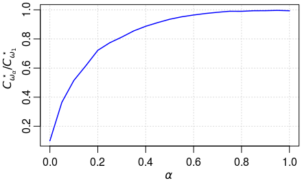
In the previous corollary, log-frequencies $\beta$ may be either strategy dependent or independent. In an uncontrolled scenario, $\beta$ is imposed by the setting and does not depend on the followed strategy, while in a controlled scenario we consider strategies that impose $\beta\!=\!1_{\mathcal{B}}\!\coloneqq\!(1)_{b\in\mathcal{B}}$ .

Like other structured bandit problems (as in Combes et al. (2017), Lattimore and Szepesvari (2017)) this lower bound is characterized by a problem-dependent constant $C_{\omega}^{\star}(\beta,\nu)$ solution to an optimization problem. In the agnostic case we recover the lower bound of the classical multi-armed bandit problem. Indeed, let us introduce for $\alpha\!\in\![0,1]$ the weight matrix $\omega_{\alpha}$ where all the weights are equal to $\alpha$ (except for the zero diagonal). $\omega_{\alpha}$ is the same weight matrix as in Figure 1 but only for one cluster. Then when there is no structure ( $\omega\!\equiv\!\omega_{1}$ ), we obtain the explicit constant

C_{\omega_{1}}^{\star}(\beta,\nu)=\sum_{b\in\mathcal{B}}\beta_{b}\!\!\sum_{a\in\mathcal{A}:\ (a,b)\notin\mathcal{O}^{\star}}\frac{\Delta_{a,b}}{\text{kl}(\mu_{a,b}|\mu_{b}^{\star})}\,,

(3)

that corresponds to solving $|\mathcal{B}|$ bandit problems in parallel (independently the ones from the others). Thus the graph structure allows to interpolate smoothly between $|\mathcal{B}|$ independent bandit problems and a unique one when all the users share the same distributions. In order to illustrate the gain of information due to the graph structure we plot in Figure 2 the expectation $\mathbb{E}_{\nu\sim\mathcal{U}(\mathcal{D}_{\omega_{\alpha}})}\!\left[C_{\omega_{\alpha}}^{\star}(1_{\mathcal{B}},\nu)/C_{\omega_{1}}^{\star}(1_{\mathcal{B}},\nu)\right]$ of the ratio between the constant in the structured case (8) and that in the agnostic case (3), where $\mathcal{U}(\mathcal{D}_{\omega_{\alpha}})$ denotes the uniform distribution over $\mathcal{D}_{\omega_{\alpha}}$ , $\alpha\!\in\![0,1]$ .

3 IMED type strategies for Graph-structured Bandits

In this section, we present for both the controlled and uncontrolled scenarios, two strategies: IMED-GS^⋆ that matches the asymptotic lower bound of Corollary 8 and IMED-GS with a lower computational complexity but weaker guaranty. Both are inspired by the Indexed Minimum Empirical Divergence (IMED) proposed by Honda and Takemura (2011). The general idea behind this algorithm is to enforce, via a well chosen index, the constraints (1) that appears in the optimization problem (8) of the asymptotic lower bound. These constraints intuitively serve as tests to assert whether or not a couple is optimal.

3.1 IMED type strategies for the controlled scenario

We consider the controlled scenario where the sequence of users $(b_{t})_{t\geqslant 1}$ is strategy-dependent and at each time step $t\!\geqslant\!1$ , the learner has to choose a user $b_{t}$ and an arm $a_{t}$ , based only on the past.

3.1.1 The IMED-GS strategy.

We denote by ${{\widehat{\mu}_{a,b}}}(t)\!=\!\frac{1}{N_{a,b}(t)}\sum\limits_{s=1}^{t}{\mathbb{I}_{\{(a_{s},b_{s})=(a,b)\}}X_{s}}$ if $N_{a,b}(t)\!>\!0$ , $0$ otherwise, the empirical mean of the rewards from couple $(a,b)$ . Guided by the lower bound (1) we generalize the IMED index to take into account the graph structure as follows. For a couple $(a,b)$ and at time $t$ we define

I_{a,b}(t)=\Bigg{\{}\begin{array}[]{ll}\log\!\left(N_{a,b}(t)\right)&\text{if }(a,b)\in\widehat{\mathcal{O}}^{\star}(t)\\ \sum\limits_{b^{\prime}\in\widehat{\mathcal{B}}_{a,b}(t)}\!\text{kl}\!\left({{\widehat{\mu}}}_{a,b^{\prime}}(t)\!\left|{{\widehat{\mu}}}_{b}^{\star}(t)-\omega_{b,b^{\prime}}\right.\!\right)\!\,N_{a,b^{\prime}}(t)+\log\!\left(N_{a,b^{\prime}}(t)\right)&\text{otherwise}\end{array}\,,

(4)

where ${{\widehat{\mu}}}_{b}^{\star}(t)\!=\!\max_{a\in\mathcal{A}}{{\widehat{\mu}_{a,b}}}(t)$ is the current best mean for user $b$ , the current set of optimal couple is

\widehat{\mathcal{O}}^{\star}(t)\coloneqq\bigg{\{}(a,b)\in\mathcal{A}\times\mathcal{B}:\ {{\widehat{\mu}_{a,b}}}(t)={{\widehat{\mu}}}_{b}^{\star}(t)\bigg{\}}

and the current set of informative users for an empirical sub-optimal couple $(a,b)$ is

\widehat{\mathcal{B}}_{a,b}(t)\coloneqq\bigg{\{}b^{\prime}\in\mathcal{B}:\ N_{a,b^{\prime}}(t)>0\text{\ \ and \ }{{\widehat{\mu}}}_{a,b^{\prime}}(t)<{{\widehat{\mu}}}_{b}^{\star}(t)-\omega_{b,b^{\prime}}\bigg{\}}\,.

This quantity can be seen as a transportation cost for “moving²²2This notion refers to the generic proof technique used to derive regret lower bounds. It involves a change-of-measure argument, from the initial configuration in which the couple is sub-optimal to another one chosen to make it optimal.” a sub-optimal couple to an optimal one, plus exploration terms (the logarithms of the numbers of pulls). When an optimal couple is considered, the transportation cost is null and only the exploration part remains. Note that, as stated in Honda and Takemura (2011), $I_{a,b}(t)$ is an index in the weaker sense since it is not determined only by samples from the couple $(a,b)$ but also uses empirical means of current optimal arms. We define IMED-GS (Indexed Minimum Empirical Divergence for Graph Structure) to be the strategy consisting of pulling a couple with minimum index in Algorithm 1. It works well in practice, see Section 4, and has a low computational complexity (proportional to the number of couples). However, it is known for other structures, see Lattimore and Szepesvari (2017), that such greedy strategy does not exploit optimally the structure of the problem. Indeed, at a high level, pulling an apparently sub-optimal couple $(a,b)$ allows to gather information not only about this particular couple but also about other couples due to the structure. In order to attain optimality one needs to find couples that provide the best trade-off between information and low regret. This is exactly what is done in the optimization problem (8).

3.1.2 The IMED-GS^⋆ strategy

In order to address this difficulty we first, thanks to the (weak) indexes, decide whether we need to exploit or explore. In the second case, in order to explore optimally according to the graph structure we solve the optimization problem (8) parametrized by the current estimates of the means and then track the optimal numbers of pulls given by the solution of this problem. More precisely at each round we choose but not immediately pull a couple with minimum index

(\underline{a}_{t},\underline{b}_{t})\in\mathop{\mathrm{argmin}}\limits_{(a,b)\in\mathcal{A}\times\mathcal{B}}I_{a,b}(t)\,.

Exploitation: If this couple is currently optimal, $(\underline{a}_{t},\underline{b}_{t})\!\in\!\widehat{\mathcal{O}}^{\star}(t)$ , we exploit, that is pull this couple.
Exploration: Else we explore arm $a_{t+1}\!=\!\underline{a}_{t}$ . To this end, let $n^{\textnormal{opt}}(t)$ be a solution of the empirical version of $\eqref{eq:lb_regret_structure}$ with $\beta=1_{\mathcal{B}}$ , that is

	$\displaystyle n^{\textnormal{opt}}(t)\in$	$\displaystyle\mathop{\mathrm{argmin}}\limits_{n\in\mathbb{R}_{+}^{\mathcal{A}\times\mathcal{B}}}$	$\displaystyle\bigg{\{}\sum\limits_{(a,b)\in\mathcal{A}\times\mathcal{B}}\big{(}{{\widehat{\mu}}}_{b}^{\star}(t)-{{\widehat{\mu}}}_{a,b}(t)\big{)}\,n_{a,b}$
		$\displaystyle s.t.$	$\displaystyle\forall(a,b)\notin\widehat{\mathcal{O}}^{\star}(t),\widehat{\mathcal{B}}_{a,b}(t)\neq\emptyset:\!\sum\limits_{b^{\prime}\in\widehat{\mathcal{B}}_{a,b}(t)}\text{kl}\!\left({{\widehat{\mu}}}_{a,b^{\prime}}(t)\!\left\|{{\widehat{\mu}}}_{b}^{\star}(t)-\omega_{b,b^{\prime}}\right.\!\right)\!\,n_{a,b^{\prime}}\geqslant 1\bigg{\}}.$

The current optimal numbers of pulls given by

N^{\textnormal{opt}}_{a,b}(t)=n^{\textnormal{opt}}_{a,b}(t)\min\limits_{b^{\prime}\in\mathcal{B}}I_{a,b^{\prime}}(t)\,.

(6)

We then track

b_{t+1}\in\mathop{\mathrm{argmax}}\limits_{b\in\widehat{\mathcal{B}}_{{\underline{a}_{t}},{\underline{b}_{t}}}(t)\cup\left\{\underline{b}_{t}\right\}}N^{\textnormal{opt}}_{\underline{a}_{t},b}(t)-N_{\underline{a}_{t},b}(t)\,.

(7)

Asymptotically, we expect that all the sub-optimal couples are pulled roughly $\log(T)$ times. Therefore, for all sub-optimal couple $(a,b)$ , the index $I_{a,b}(T)$ should be of order $\log(T)$ . Thus we asymptotically recover in the definition of $N^{\textnormal{opt}}_{a,b}(\cdot)$ the optimal number of pulls of couple $(a,b)$ , that is $n^{\nu}_{a,b}\log(T)$ as suggested in Corollary 8. Finally we pull the selected couple $(a_{t+1},b_{t+1})$ . In order to ensure optimality, however, such a direct tracking of the current optimal number of pulls is still a bit too aggressive and we need to force exploration in some exploration rounds. We proceed as follows: when we explore arm $\underline{a}_{t}$ we automatically pull a couple $(\underline{a}_{t},b)$ if its number of pulls $N_{\underline{a}(t),b}$ is lower than the logarithm of the number of time we decided to explore this arm. See Algorithm 2 for details. This does not hurt the asymptotic optimally because we expect to explore a sub-optimal arm not more than $\log(T)$ times. On the bright side, this is still different than the traditional forced exploration. Indeed, only few rounds are dedicated to exploration thanks to the first selection with the indexes and among them only a logarithmic number will consist of pure exploration: Thus, we expect an overall $\log\log(T)$ rounds of forced exploration. Note also that all the quantities involved in this forced exploration use empirical counters. Putting all together we end up with strategy IMED-GS^⋆ described in Algorithm 2.

Comparison with other strategies

IMED-GS^⋆ combines ideas from IMED introduced by Honda and Takemura (2011) and from OSSB by Combes et al. (2017). More precisely, it generalizes the index from IMED to the graph structure. From OSSB it borrows the tracking of the optimal counts given by the asymptotic lower bound (see also Lattimore and Szepesvari (2017)) and the way to force exploration sparingly. The main difference with OSSB is that IMED-GS^⋆ leverages the indexes to deal with the exploitation-exploration trade-off. In particular IMED-GS^⋆ does not need to solve at each round the optimization problem (8). This greatly improves the computational complexity. Also, note that OSSB requires choosing a tuning parameter that must be positive to ensure theoretical guarantees but that must be set equal to $0$ to work well in practice. This is not the case for IMED-GS^⋆ that requires no parameter tuning and that works well both in theory and in practice (see Section 4).

Algorithm 1 IMED-GS (controlled scenario) 0: Weight matrix $(\omega_{b,b^{\prime}})_{b,b^{\prime}\in\mathcal{B}}$ . for $t=1...T$ do Pull $(a_{t+1},b_{t+1})\!\in\!\mathop{\mathrm{argmin}}\limits_{(a,b)\in\mathcal{A}\times\mathcal{B}}\!I_{a,b}(t)$ end for Algorithm 2 IMED-GS^⋆ (controlled scenario) 0: Weight matrix $(\omega_{b,b^{\prime}})_{b,b^{\prime}\in\mathcal{B}}$ . $\forall a\in\mathcal{A},\quad c_{a},c_{a}^{+}\leftarrow 1$ for For $t=1...T$ do Choose $(\underline{a}_{t},\underline{b}_{t})\in\mathop{\mathrm{argmin}}\limits_{(a,b)\in\mathcal{A}\times\mathcal{B}}I_{a,b}(t)$ if $(\underline{a}_{t},\underline{b}_{t})\in\widehat{\mathcal{O}}^{\star}(t)$ then Choose $(a_{t+1},b_{t+1})=(\underline{a}_{t},\underline{b}_{t})$ else Set $a_{t+1}=\underline{a}_{t}$ if $c_{a_{t+1}}=c_{a_{t+1}}^{+}$ then $c_{a_{t+1}}^{+}\leftarrow 2c_{a_{t+1}}^{+}$ Choose $b_{t+1}\in\mathop{\mathrm{argmin}}\limits_{b\in\mathcal{B}}N_{a,b}(t)$ else Choose $b_{t+1}\!\!\in\!\!\!\!\!\mathop{\mathrm{argmax}}\limits_{b\in\widehat{\mathcal{B}}_{{\underline{a}_{t}},{\underline{b}_{t}}}(t)\cup\left\{\underline{b}_{t}\right\}}\!\!\!\!\!\!N^{\textnormal{opt}}_{a_{t+1},b}(t)\!-\!N_{a_{t+1},b}(t)$ end if $c_{a_{t+1}}\leftarrow c_{a_{t+1}}+1$ end if Pull $(a_{t+1},b_{t+1})$ end for

3.2 IMED type strategies for the uncontrolled scenario

In this section, an uncontrolled scenario is considered where the sequence of users $(b_{t})_{t\geqslant 1}$ is assumed deterministic and does not depend on the strategy of the learner. We adapt the two previous strategies IMED-GS and IMED-GS^⋆ to this scenario.

IMED-GS₂ strategy

At time step $t\!\geqslant\!1$ the choice of user $b_{t}$ is no longer strategy-dependent but is imposed by the sequence of users $(b_{t})_{t\geqslant 1}$ which is assumed to be deterministic in the uncontrolled scenario. The learner only chooses an arm to pull $a_{t}$ knowing user $b_{t}$ . We define IMED-GS₂ to be the strategy consisting of pulling an arm with minimum index in Algorithm 3 of Appendix C. IMED-GS₂ suffers the same advantages and shortcomings as IMED-GS. It does not exploit optimally the structure of the problem but it works well in practice, see Section 4, and has a low computational complexity.

IMED-GS ${}^{\star}_{2}$ strategy

In order to explore optimally according to the graph structure in the uncontrolled scenario, we also track the optimal numbers of pulls. $\beta$ may be at first glance different from $1_{\mathcal{B}}$ . This requires some normalizations. First, for all time step $t\!\geqslant\!1$ , $n^{\textnormal{opt}}(t)$ now denotes a solution of the empirical version of $\eqref{eq:lb_regret_structure}$ with $\beta\!=\!(\widehat{\beta}_{b}(t))_{b\in\mathcal{B}}$ where $\widehat{\beta}_{b}(t)\!=\!\!\log\!\left(N_{b}(t)\right)\!/\log(t)$ estimates log-frequency $\beta_{b}$ of user $b\!\in\!\mathcal{B}$ . Second, we have to consider normalized indexes $\widetilde{I}_{a,b}(t)\!=\!I_{a,b}(t)/\widehat{\beta}_{b}(t)$ for couples $(a,b)\!\in\!\mathcal{A}\!\times\!\mathcal{B}$ in order to have $\widetilde{I}_{a,b}(T)\!\sim\!\log(T)$ as in the controlled scenario. An additional difficulty is that at a given time step $t\!\geqslant\!1$ , while the indexes indicate to explore, the current tracked user (see Equation 7) given is likely to be different from user $b_{t}$ with whom the learner deals. This difficulty is easy to circumvent by postponing and prioritizing the exploration until the learner deals with the tracked user. Priority in exploration phases is given to first delayed forced-exploration and delayed exploration based on solving optimization problem (8), then exploration based on current indexes (see Algorithm 4 in Appendix C). IMED-GS ${}^{\star}_{2}$ corresponds essentially to IMED-GS^⋆ with some delays due to the fact that the tracked and the current users may be different. This has no impact on the optimality of IMED-GS ${}^{\star}_{2}$ since log-frequencies of users are enforced to be positive.

3.3 Asymptotic optimality of IMED type strategies

In order to prove the asymptotic optimality of IMED-GS^⋆ we introduce the following mild assumptions on the configuration considered.

Definition 10 (Non-peculiar configuration)

A configuration $\nu\!\in\!\mathcal{D}_{\omega}$ is non-peculiar if the optimization problem (8) admits a unique solution and each user $b$ admits a unique optimal arm $a_{b}^{\star}$ .

In Theorem 11 we state the main result of this paper, namely, the asymptotic optimality of IMED-GS^⋆ and IMED-GS ${}^{\star}_{2}$ . We prove this result for IMED-GS^⋆ in Appendix E and adapt this proof in Appendix G for IMED-GS ${}^{\star}_{2}$ . Please refer to Proposition 20 (Appendix D) for more refined finite-time upper bounds. As a byproduct of this analysis we deduce the Pareto-optimality of IMED-GS and IMED-GS₂ stated in Proposition 12 and proved in Appendix G.

Theorem 11 (Asymptotic optimality)

Both IMED-GS^⋆ and IMED-GS ${}^{\star}_{2}$ are consistent strategies. Further, they are asymptotically optimal on the set of non-peculiar configurations, that is, for all $\nu\in\mathcal{D}_{\omega}$ non-peculiar, under IMED-GS^⋆ the sequence of users has log-frequencies $1_{\mathcal{B}}$ and we have

\limsup\limits_{T\rightarrow\infty}\dfrac{R(\nu,T)}{\log(T)}\leqslant C_{\omega}^{\star}(1_{\mathcal{B}},\nu)\,,

and, under IMED-GS ${}^{\star}_{2}$ , assuming a sequence of users with log-frequencies $\beta\!\in\!(0,1]^{\mathcal{B}}$ , we have

\limsup\limits_{T\rightarrow\infty}\dfrac{R(\nu,T)}{\log(T)}\leqslant C_{\omega}^{\star}(\beta,\nu)\,.

Proposition 12 (Asymptotic Pareto-optimality)

Both IMED-GS and IMED-GS₂ are consistent strategies. Further, they are asymptotically Pareto-optimal on the set of non-peculiar configurations, that is, under IMED-GS or IMED-GS₂, for all $\nu\in\mathcal{D}_{\omega}$ non-peculiar,

\forall a\in\mathcal{A},\quad\limsup\limits_{T\rightarrow\infty}\min\limits_{b:\ (a,b)\notin\mathcal{O}^{\star}}\frac{1}{\log\!\left(N_{b}(T)\right)}\sum\limits_{b^{\prime}\in\mathcal{B}_{a,b}}\text{kl}(\mu_{a,b^{\prime}}|\mu_{b}^{\star}-\omega_{b,b^{\prime}})N_{a,b^{\prime}}(T)\leqslant 1\,.

Discussion

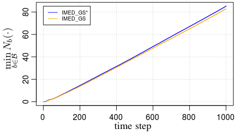
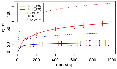
Removing forced exploration remains the most challenging task for structured bandit problems. In the context of this structure, forced exploration would have been to use criteria like "if $N_{a,b}(T)\!<\!\widehat{c}_{a,b}(T)\log(T)$ , then pull couple $(a,b)$ " for some constants $\widehat{c}_{a,b}(T)$ that depends on the minimization problem coming from the lower bound and where $\widehat{c}_{a,b}(T)\log(T)$ can be interpreted as an estimator of the theoretical asymptotic lower bound on the numbers of pulls of couple $(a,b)$ . In stark contrast, in IMED-GS^⋆ there is no forced exploration in choosing the arm to explore and, in choosing the user to explore, the used criteria is more intrinsic as it reads "if $N_{a,b}(T)\!<\!\widehat{c}_{a,b}(T)I_{a}(T)$ , then pull couple $(a,b)$ ", where $I_{a}(T)\!\sim\!\log(T)$ but really depends on $(N_{a,b}(T))_{(a,b)\notin\mathcal{C}^{\star}}$ . Thus, the used criteria are not asymptotic, and do not dependent on the time $t$ but on the current numbers of pull of sub-optimal arms. Since theoretical asymptotic lower bounds on the numbers of pulls are significantly larger than the current numbers of pulls in finite horizon (see Figure 3), IMED-GS^⋆ strategy is also expected to behave better than strategies based on usual (conservative) forced exploration. Although entirely removing forced exploration would be nicer, in IMED-GS^⋆, forced exploration is only done in a sparing way.

4 Numerical experiments

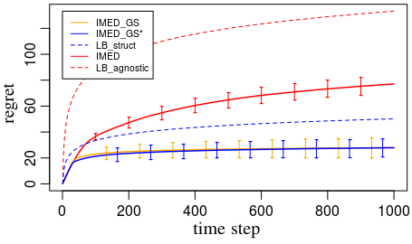
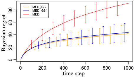
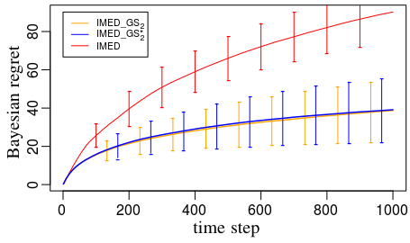
In this section, we compare empirically the following strategies introduced beforehand: IMED-GS and IMED-GS^⋆ described respectively in Algorithms 1, 2, IMED-GS₂ and IMED-GS ${}^{\star}_{2}$ described respectively in Algorithms 3, 4 and the baseline IMED by Honda and Takemura (2011) that does not exploit the structure. We compare these strategies on two setups, each with $|\mathcal{B}|\!=\!10$ users and $|\mathcal{A}|\!=\!5$ arms. For the uncontrolled scenario we consider the round-robin sequence of users. As expected the strategies leveraging the graph structure perform better than the baseline IMED that does not exploit it. Furthermore, the plots suggest that IMED-GS and IMED-GS^⋆ (respectively IMED-GS₂ and IMED-GS ${}^{\star}_{2}$ ) perform similarly in practice.

Fixed configuration

Figure 3: Left – For these experiments we investigate these strategies on a fixed configuration. The weight matrix $\omega$ and the configuration $\nu\!\in\!\mathcal{D}_{\omega}$ are given in Appendix I. This enables us to plot also the asymptotic lower bound on the regret for reference: We plot the unstructured lower bound (LB_agnostic) in dashed red line, and the structured lower bound (LB_struct) in dashed blue line.

Random configurations

Figure 3: Right – In these experiments we average regrets over random configurations. We proceed as follows: At each run we sample uniformly at random a weight matrix $\omega$ and then sample uniformly at random a configuration $\nu\!\in\!\mathcal{D}_{\omega}$ .

Additional experiments in Appendix I confirm that both IMED-GS and IMED-GS^⋆ induce sequences of users with log-frequencies all equal to $1$ .

Acknowledgments

This work was supported by CPER Nord-Pas de Calais/FEDER DATA Advanced data science and technologies 2015-2020, the French Ministry of Higher Education and Research, the French Agence Nationale de la Recherche (ANR) under grant ANR-16- CE40-0002 (project BADASS), and Inria Lille – Nord Europe.

A Notations and reminders

For $\nu\in\mathcal{D}_{\nu}$ , we define

\varepsilon_{\nu}\coloneqq\min\limits_{\begin{subarray}{c}(a,b)\notin\mathcal{O}^{\star},b^{\prime}\in\mathcal{B}\\ \mu_{a,b^{\prime}}-\mu_{b}^{\star}-\omega_{b,b^{\prime}}\neq 0\end{subarray}}\left\{\dfrac{\left|\mu_{a,b^{\prime}}-\mu_{b}^{\star}-\omega_{b,b^{\prime}}\right|}{4},\dfrac{\mu_{a,b}}{4},\dfrac{1-\mu_{b}^{\star}}{4}\right\}\,.

Then, there exists $\alpha_{\nu}:\mathbb{R}_{+}^{\star}\to\mathbb{R}_{+}^{\star}$ such that $\lim\limits_{\varepsilon\to 0}\alpha_{\nu}(\varepsilon)=0$ and such that for all $0<\varepsilon<\varepsilon_{\nu}$ , for all $(a,b)\notin\mathcal{O}^{\star}$ , for all $b^{\prime}\in\mathcal{B}$ ,

\mu_{a,b^{\prime}}\neq\mu_{b}^{\star}-\omega_{b,b^{\prime}}\quad\Rightarrow\quad\dfrac{\text{kl}(\mu_{a,b^{\prime}}|\mu_{b}^{\star}-\omega_{b,b^{\prime}})}{1+\alpha_{\nu}(\varepsilon)}\!\leqslant\!\text{kl}(\mu_{a,b^{\prime}}\pm\varepsilon|\mu_{b}^{\star}-\omega_{b,b^{\prime}}\pm\varepsilon)\!\leqslant\!(1+\alpha_{\nu}(\varepsilon))\text{kl}(\mu_{a,b^{\prime}}|\mu_{b}^{\star}-\omega_{b,b^{\prime}})\,.

We also introduce the following constant of interest

E_{\nu}\coloneqq 6e\,\max\limits_{a\in\mathcal{A},b\in\mathcal{B}}\left(1-\frac{\log(1-\mu_{a,b}-\varepsilon_{\nu})}{\log(1-\mu_{a,b})}\right)^{-1}\left(1-e^{-\!\left(1-\frac{\log(1-\mu_{a,b}-\varepsilon_{\nu})}{\log(1-\mu_{a,b})}\right)\text{kl}(\mu_{a,b}|\mu_{a,b}-\varepsilon_{\nu})}\right)^{-3}\,.

Lastly, for all couple $(a,b)\in\mathcal{A}\times\mathcal{B}$ , for all $n\geqslant 1$ , we consider the stopping times

\tau_{a,b}^{n}\coloneqq\inf{\left\{t\!\geqslant\!1\!:N_{a,b}(t)\!=\!n\right\}}

and define

{{\widehat{\mu}_{a,b}}}^{n}\!\coloneqq\!{{\widehat{\mu}_{a,b}}}(\tau_{a,b}^{n})\,.

B Proof related to the regret lower bound (Section 2)

In this section we regroup the proofs related to the lower bounds.

B.1 Almost sure asymptotic lower bounds under consistent strategies

In this section we prove Proposition 5.

Let us consider a consistent strategy on $\mathcal{D}_{\omega}$ . Let $\nu\in\mathcal{D}_{\omega}$ and let us consider $(a,b)\notin\mathcal{O}^{\star}$ . We show that almost surely $\lim\limits_{T\to\infty}N_{b}(T)=+\infty$ implies

\liminf\limits_{T\rightarrow\infty}\dfrac{1}{\log\!\left(N_{b}(T)\right)}\sum\limits_{b^{\prime}\in\mathcal{B}_{a,b}}N_{a,b^{\prime}}(T)\text{kl}(\mu_{a,b^{\prime}}|\mu_{b}^{\star}-\omega_{b,b^{\prime}})\geqslant 1\,

where $\mathcal{B}_{a,b}=\left\{b^{\prime}\in\mathcal{B}:\ (a,b^{\prime})\notin\mathcal{O}^{\star}\text{\ \ and \ }\mu_{a,b^{\prime}}<\mu_{b}^{\star}-\omega_{b,b^{\prime}}\right\}$ .

Proof Let us consider $\widetilde{\nu}\in\mathcal{D}_{\omega}$ , a maximal confusing distribution for the sub-optimal couple $(a,b)$ such that $a$ is the unique optimal arm of user $b$ for $\widetilde{\nu}$ , defined as follows:

-

$\forall a^{\prime}\neq a,\ b^{\prime}\in\mathcal{B},\quad\widetilde{\mu}_{a^{\prime},b^{\prime}}=\mu_{a^{\prime},b^{\prime}}$
-

$\forall b^{\prime\prime}\notin\mathcal{B}_{a,b},\quad\widetilde{\mu}_{a,b^{\prime\prime}}=\mu_{a,b^{\prime\prime}}$
-

$\forall b^{\prime}\in\mathcal{B}_{a,b},\quad\widetilde{\mu}_{a,b^{\prime}}=\mu_{b}^{\star}-\omega_{b,b^{\prime}}+\varepsilon$

where $0<\varepsilon<\varepsilon_{0}=\min\limits_{b^{\prime}\in\mathcal{B}}\left|\mu_{b}^{\star}-\omega_{b,b^{\prime}}-\mu_{a,b^{\prime}}\right|$ . Our assumption on $\mathcal{D}_{\omega}\subset\overline{\mathcal{D}}_{\omega}$ ensures that $\varepsilon_{0}>0$ . Note that $\varepsilon$ is chosen in such a way that for all $b^{\prime},b^{\prime\prime}\in\mathcal{B}$ , $\max\limits_{a\in\mathcal{A}}\left|\widetilde{\mu}_{a,b^{\prime}}-\widetilde{\mu}_{a,b^{\prime\prime}}\right|\leqslant\omega_{b^{\prime},b^{\prime\prime}}$ . Indeed we have:
- for $b^{\prime},b^{\prime\prime}\in\mathcal{B}_{a,b}:\quad\left|\widetilde{\mu}_{a,b^{\prime}}-\widetilde{\mu}_{a,b^{\prime\prime}}\right|=\left|\omega_{b,b^{\prime}}-\omega_{b,b^{\prime\prime}}\right|\leqslant\omega_{b^{\prime},b^{\prime\prime}}$
- for $b^{\prime},b^{\prime\prime}\notin\mathcal{B}_{a,b}:\quad\left|\widetilde{\mu}_{a,b^{\prime}}-\widetilde{\mu}_{a,b^{\prime\prime}}\right|=\left|\mu_{a,b^{\prime}}-\mu_{a,b^{\prime\prime}}\right|\leqslant\omega_{b^{\prime},b^{\prime\prime}}$
- for $b^{\prime}\in\mathcal{B}_{a,b}$ and $b^{\prime\prime}\notin\mathcal{B}_{a,b}$ , we have $\widetilde{\mu}_{a,b^{\prime}}-\widetilde{\mu}_{a,b^{\prime\prime}}=\mu_{b}^{\star}-\omega_{b,b^{\prime}}+\varepsilon-\mu_{a,b^{\prime\prime}}$ . Since in this case $b^{\prime}\in\mathcal{B}_{a,b}$ it implies $\mu_{a,b^{\prime}}\leqslant\mu_{b}^{\star}-\omega_{b,b^{\prime}}$ and since $b^{\prime\prime}\notin\mathcal{B}_{a,b}:\mu_{a,b^{\prime\prime}}\geqslant\mu_{b}^{\star}-\omega_{b,b^{\prime\prime}}+\varepsilon_{0}$ . Therefore on one hand we get

\mu_{b}^{\star}-\omega_{b,b^{\prime}}+\varepsilon-\mu_{a,b^{\prime\prime}}\geqslant\mu_{a,b^{\prime}}-\mu_{a,b^{\prime\prime}}\geqslant-\omega_{b^{\prime},b^{\prime\prime}}\,,

and on the other hand

\mu_{b}^{\star}-\omega_{b,b^{\prime}}+\varepsilon-\mu_{a,b^{\prime\prime}}\leqslant\mu_{b}^{\star}-\omega_{b,b^{\prime}}+\varepsilon-(\mu_{b}^{\star}-\omega_{b,b^{\prime\prime}}+\varepsilon_{0})=\varepsilon-\varepsilon_{0}+\omega_{b,b^{\prime\prime}}-\omega_{b,b^{\prime}}\leqslant\omega_{b^{\prime},b^{\prime\prime}}\,.

Actually, we can choose $0<\varepsilon<\varepsilon_{\nu}$ so that :

\forall b^{\prime}\in\mathcal{B}_{a,b},\ \text{kl}(\mu_{a,b^{\prime}}|\widetilde{\mu}_{a,b^{\prime}})\leqslant(1+\alpha_{\nu}(\varepsilon))\text{kl}(\mu_{a,b^{\prime}}|\mu_{b}^{\star}-\omega_{b,b^{\prime}}).

We refer to Appendix A for the definitions of $\varepsilon_{\nu}$ and $\alpha_{\nu}(\cdot)$ . Note that $\alpha_{\nu}(\cdot)$ is such that $\lim\limits_{\varepsilon\to 0}\alpha_{\nu}(\varepsilon)=0$ .

Let $0<c<1$ .We will show that almost surely $\lim\limits_{T\to\infty}N_{b}(T)=+\infty$ implies

\liminf\limits_{T\rightarrow\infty}\dfrac{1}{\log\!\left(N_{b}(T)\right)}\sum\limits_{b^{\prime}\in\mathcal{B}_{a,b}}N_{a,b^{\prime}}(T)\text{kl}(\mu_{a,b^{\prime}}|\widetilde{\mu}_{a,b^{\prime}})\geqslant c\,.

We start with the following inequality

	$\displaystyle\mathbb{P}_{\nu}\!\left(\liminf\limits_{T\rightarrow\infty}\dfrac{1}{\log\!\left(N_{b}(T)\right)}\sum\limits_{b^{\prime}\in\mathcal{B}_{a,b}}N_{a,b^{\prime}}(T)\text{kl}(\mu_{a,b^{\prime}}\|\widetilde{\mu}_{a,b^{\prime}})<c,\ \lim\limits_{T\rightarrow\infty}N_{b}(T)=\infty\right)$
			$\displaystyle\leqslant\liminf\limits_{T\rightarrow\infty}\mathbb{P}_{\nu}\!\left(\dfrac{1}{\log\!\left(N_{b}(T)\right)}\sum\limits_{b^{\prime}\in\mathcal{B}_{a,b}}N_{a,b^{\prime}}(T)\text{kl}(\mu_{a,b^{\prime}}\|\widetilde{\mu}_{a,b^{\prime}})<c,\ \lim\limits_{T\rightarrow\infty}N_{b}(T)=\infty\right)\,.$

Let us consider an horizon $T\geqslant 1$ and let us introduce the event

\Omega_{T}=\left\{\sum\limits_{b^{\prime}\in\mathcal{B}_{a,b}}N_{a,b^{\prime}}(T)\text{kl}(\mu_{a,b^{\prime}}|\widetilde{\mu}_{a,b^{\prime}})<c\log\!\left(N_{b}(T)\right),\ \lim\limits_{T\rightarrow\infty}N_{b}(T)=\infty\right\}.

We want to provide an upper bound on $\mathbb{P}_{\nu}(\Omega_{T})$ to ensure $\lim\limits_{T\rightarrow\infty}\!\mathbb{P}_{\nu}(\Omega_{T})=0$ . We start by taking advantage of the following lemma.

Lemma 13 (Change of measure)

For every event $\Omega$ and random variable $Z$ both measurable with respect to $\nu$ and $\widetilde{\nu}$ ,

\mathbb{P}_{\nu}(\Omega\cap E)=\mathbb{E}_{\widetilde{\nu}}\!\left[\dfrac{\textnormal{ d}\nu}{\textnormal{ d}\widetilde{\nu}}(\psi)\mathbb{I}_{\left\{\Omega\cap E\right\}}\right]\leqslant\mathbb{E}_{\widetilde{\nu}}\!\left[e^{Z}\mathbb{I}_{\left\{\Omega\right\}}\right]

where $E=\left\{\log\left(\dfrac{\textnormal{ d}\nu}{\textnormal{ d}\widetilde{\nu}}(\psi)\right)\leqslant Z\right\}$ and $\psi=((a_{t},b_{t}),X_{t})_{t=1..T}$ is the sequence of pulled couples and rewards.

Let $\alpha\in(0,1)$ and let us introduce the event

E_{T}=\left\{\log\left(\dfrac{\textnormal{ d}\nu}{\textnormal{ d}\widetilde{\nu}}(\psi)\right)\leqslant(1-\alpha)\log\!\left(N_{b}(T)\right)\right\}.

Then we can decompose the probability as follows

\mathbb{P}_{\nu}(\Omega_{T})=\mathbb{P}_{\nu}(\Omega_{T}\cap E_{T})+\mathbb{P}_{\nu}(\Omega_{T}\cap E_{T}^{c})\leqslant\mathbb{E}_{\widetilde{\nu}}\!\left[N_{b}(T)^{1-\alpha}\mathbb{I}_{\left\{\Omega_{T}\right\}}\right]+\mathbb{P}_{\nu}(\Omega_{T}\cap E_{T}^{c})

Now, we control successively $\mathbb{E}_{\widetilde{\nu}}\!\left[N_{b}(T)^{1-\alpha}\mathbb{I}_{\left\{\Omega_{T}\right\}}\right]$ and $\mathbb{P}_{\nu}(\Omega_{T}\cap E_{T}^{c})$ and show that they both tend to $0$ as $T$ tends to $\infty$ .

B.1.1 $\mathbb{E}_{\widetilde{\nu}}\!\left[N_{b}(T)^{1-\alpha}\mathbb{I}_{\left\{\Omega_{T}\right\}}\right]$ tends to $0$ when $T$ tends to infinity

We first provide an upper bound on $\mathbb{I}_{\left\{\Omega_{T}\right\}}$ as follows, denoting $c^{\prime}=c/\text{kl}(\mu_{a,b^{\prime}}|\widetilde{\mu}_{a,b^{\prime}})$ ,

	$\displaystyle\Omega_{T}$	$\displaystyle\subset$	$\displaystyle\left\{N_{a,b}(T)<c^{\prime}\log\!\left(N_{b}(T)\right),\ \lim\limits_{T\rightarrow\infty}N_{b}(T)=\infty\right\}$
		$\displaystyle=$	$\displaystyle\left\{N_{b}(T)<c^{\prime}\log\!\left(N_{b}(T)\right)+\sum\limits_{a^{\prime}\neq a}N_{a^{\prime},b}(T),\ \lim\limits_{T\rightarrow\infty}N_{b}(T)=\infty\right\}\,.$

Thus, we have

\mathbb{I}_{\left\{\Omega_{T}\right\}}\leqslant c^{\prime}\mathbb{I}_{\left\{N_{b}(T)\geqslant 1,\ N_{b}(T)\to\infty\right\}}\dfrac{\log\!\left(N_{b}(T)\right)}{N_{b}(T)}+\sum\limits_{a^{\prime}\neq a}\dfrac{N_{a^{\prime},b}(T)}{N_{b}(T)}

Considering $f_{\alpha}\!:x\!\geqslant\!1\!\mapsto\!\log(x)/x^{\alpha}$ , we have $f_{\alpha}\!\leqslant\!e^{-1}/\alpha$ . Then, the dominated convergence theorem ensures

\mathbb{E}_{\widetilde{\nu}}\!\left[\mathbb{I}_{\left\{N_{b}(T)\geqslant 1,\ N_{b}(T)\to\infty\right\}}\dfrac{\log\!\left(N_{b}(T)\right)}{N_{b}(T)^{\alpha}}\right]=o(1)\,.

Furthermore, since the considered strategy is assumed consistent we know that for $a^{\prime}\neq a$ , since $a^{\prime}$ is a sub-optimal arm for user $b$ and configuration $\widetilde{\nu}$ ,

\mathbb{E}_{\widetilde{\nu}}\!\left[\dfrac{N_{a,b^{\prime}}(T)}{N_{b}(T)^{\alpha}}\right]=o(1)\,,

therefore we get

\mathbb{E}_{\widetilde{\nu}}\!\left[N_{b}(T)^{1-\alpha}\mathbb{I}_{\left\{\Omega_{T}\right\}}\right]=o(1).

B.1.2 $\mathbb{P}_{\nu}(\Omega_{T}\cap E_{T}^{c})$ tends to $0$ when $T$ tends to infinity

For each time $t=1,\ldots,T$ , the reward $X_{t}$ is sampled independently from the past and according to $\nu_{a_{t},b_{t}}$ . Hence the likelihood ratio rewrites

\dfrac{\textnormal{ d}\nu}{\textnormal{ d}\widetilde{\nu}}(\psi)=\prod_{t=1}^{T}\dfrac{\textnormal{ d}\nu_{a_{t},b_{t}}}{\textnormal{ d}\widetilde{\nu}_{a_{t},b_{t}}}(X_{t})

where, for all $(a,b)\in\mathcal{A}\times\mathcal{B}$ and for all $x\in\left\{0,1\right\}$ , we have : $\dfrac{\textnormal{ d}\nu_{a,b}}{\textnormal{ d}\widetilde{\nu}_{a,b}}(x)=\dfrac{\mu_{a,b}^{x}(1-\mu_{a,b})^{1-x}}{\widetilde{\mu}_{a,b}^{x}(1-\widetilde{\mu}_{a,b})^{1-x}}$ .
Thus, since for all $b^{\prime}\notin\mathcal{B}_{a,b},\ \mu_{a,b}=\widetilde{\mu}_{a,b}$ , the log-likelihood ratio is

\log\left(\dfrac{\textnormal{ d}\nu}{\textnormal{ d}\widetilde{\nu}}(\psi)\right)=\sum\limits_{b^{\prime}\in\mathcal{B}_{a,b}}\sum_{t=1}^{T}\mathbb{I}_{\left\{(a_{t},b_{t})=(a,b^{\prime})\right\}}\log\left(\dfrac{\textnormal{ d}\nu_{a,b^{\prime}}}{\textnormal{ d}\widetilde{\nu}_{a,b^{\prime}}}(X_{t})\right)\,.

Let us introduce, for $(a,b)\in\mathcal{A}\times\mathcal{B}$ , $X_{a,b}^{n}=X_{\tau_{a,b}^{n}}$ where $\tau_{a,b}^{n}=\min\left\{t\geqslant 1\text{\ \ s.t. \ }N_{a,b}(t)=n\right\}$ . Note that the random variables $\tau_{a,b}^{n}$ are predictable stopping times, since $\left\{\tau_{a,b}^{n}=t\right\}$ is measurable with respect to the filtration generated by $((a_{1},b_{1}),X_{1},...,(a_{t-1},b_{t-1}),X_{t-1})$ . Hence we can rewrite the event $E_{T}$

E_{T}=\left\{\sum\limits_{b^{\prime}\in\mathcal{B}_{a,b}}\sum\limits_{t=1}^{T}\mathbb{I}_{\left\{(a_{t},b_{t})=(a,b)\right\}}\dfrac{\textnormal{ d}\nu_{a,b^{\prime}}}{\textnormal{ d}\widetilde{\nu}_{a,b^{\prime}}}(X_{t})\leqslant(1-\alpha)\log\!\left(N_{b}(T)\right)\right\}

and, since $\Omega_{T}=\left\{\sum\limits_{b^{\prime}\in\mathcal{B}_{a,b}}N_{a,b^{\prime}}(T)\text{kl}(\mu_{a,b^{\prime}}|\widetilde{\mu}_{a,b^{\prime}})<c\log\!\left(N_{b}(T)\right),\ \lim\limits_{T\rightarrow\infty}N_{b}(T)=\infty\right\}$ , we have

	$\displaystyle\Omega_{T}\cap E_{T}^{c}$	$\displaystyle\subset\bigg{\{}\exists(n_{b^{\prime}})_{b^{\prime}\in\mathcal{B}_{a,b}}:\ \sum\limits_{b^{\prime}\in\mathcal{B}_{a,b}}n_{b^{\prime}}\text{kl}(\mu_{a,b^{\prime}}\|\widetilde{\mu}_{a,b^{\prime}})<c\log\!\left(N_{b}(T)\right),\ \lim\limits_{T\rightarrow\infty}N_{b}(T)=\infty$
		$\displaystyle\textnormal{ and }\sum\limits_{b^{\prime}\in\mathcal{B}_{a,b}}\sum\limits_{n=1..n_{b^{\prime}}}\dfrac{\textnormal{ d}\nu_{a,b^{\prime}}}{\textnormal{ d}\widetilde{\nu}_{a,b^{\prime}}}(X_{a,b^{\prime}}^{n})>(1-\alpha)\log\!\left(N_{b}(T)\right)$	$\displaystyle\bigg{\}}\,.$

For $b^{\prime}\in\mathcal{B}_{a,b}$ and $n\geqslant 1$ , let us consider $Z_{b^{\prime}}^{n}=\dfrac{\textnormal{ d}\nu_{a,b^{\prime}}}{\textnormal{ d}\widetilde{\nu}_{a,b^{\prime}}}(X_{a,b^{\prime}}^{n})$ . Then $Z_{b^{\prime}}^{n}$ is positive and bounded by $B_{b^{\prime}}=\dfrac{1}{\widetilde{\mu}_{a,b^{\prime}}(1-\widetilde{\mu}_{a,b^{\prime}})}$ , with mean $\mathbb{E}_{\nu}[Z_{b^{\prime}}^{n}]=\text{kl}(\mu_{a,b^{\prime}}|\widetilde{\mu}_{a,b^{\prime}})$ . Furthermore, the random variables $Z_{b^{\prime}}^{n}$ , for $b^{\prime}\in\mathcal{B}_{a,b}$ and $n\geqslant 1$ , are independent. Thus, it holds

\Omega_{T}\cap E_{T}^{c}\subset\left\{\max\limits_{(n_{b}^{\prime})\in\mathcal{N}_{a,b}}\sum\limits_{b^{\prime}\in\mathcal{B}_{a,b}}\sum\limits_{n=1..n_{b^{\prime}}}\!\!\!\!\!Z_{b^{\prime}}^{n}-\mathbb{E}_{\nu}[Z_{b^{\prime}}^{n}]>\left(\dfrac{1-\alpha}{c}-1\right)c\log\!\left(N_{b}(T)\right),\ N_{b}(T)\!\to\!\infty\!\right\},

where

\mathcal{N}_{a,b}\coloneqq\left\{(n_{b^{\prime}})_{b^{\prime}\in\mathcal{B}_{a,b}}:\ \sum\limits_{b^{\prime}\in\mathcal{B}_{a,b}}n_{b^{\prime}}\text{kl}(\mu_{a,b^{\prime}}|\widetilde{\mu}_{a,b^{\prime}})<c\log(T)\right\}.

In the following, we apply Doob’s maximal inequality. For $b^{\prime}\in\mathcal{B}_{a,b}$ and $\lambda>0$ , let us introduce the super-martingale

M_{n}^{b^{\prime}}=\exp\!\left(\lambda\sum\limits_{k=1}^{n}\big{(}Z_{b^{\prime}}^{k}-E[Z_{b^{\prime}}^{k}]\big{)}-n\lambda^{2}\dfrac{B_{b^{\prime}}^{2}}{8}\right).

Then noting that

\dfrac{\sum\limits_{b^{\prime}\in\mathcal{B}_{a,b}}\lambda^{2}n_{b^{\prime}}\frac{B_{b^{\prime}}^{2}}{8}}{c\log(T)}<\dfrac{\sum\limits_{b^{\prime}\in\mathcal{B}_{a,b}}\lambda^{2}n_{b^{\prime}}\frac{B_{b^{\prime}}^{2}}{8}}{\sum\limits_{b^{\prime}\in\mathcal{B}_{a,b}}n_{b^{\prime}}\text{kl}(\mu_{a,b^{\prime}}|\widetilde{\mu}_{a,b^{\prime}})}\leqslant\lambda^{2}\dfrac{\max\limits_{b^{\prime}\in\mathcal{B}_{a,b}}B_{b^{\prime}}^{2}}{8\min\limits_{b^{\prime}\in\mathcal{B}_{a,b}}\text{kl}(\mu_{a,b^{\prime}}|\widetilde{\mu}_{a,b^{\prime}})}\,,

we obtain

	$\displaystyle\Omega_{T}\cap E_{T}^{c}$	$\displaystyle\subset$	$\displaystyle\left\{\max\limits_{(n_{b}^{\prime})\in\mathcal{N}_{a,b}}\prod\limits_{b^{\prime}\in\mathcal{B}_{a,b}}M_{n_{b}^{\prime}}^{b^{\prime}}>T^{\Big{[}\lambda(\frac{1-\alpha}{c}-1)-\lambda^{2}\frac{\max_{b^{\prime}\in\mathcal{B}_{a,b}}B_{b^{\prime}}^{2}}{8\min_{b^{\prime}\in\mathcal{B}_{a,b}}\text{kl}(\mu_{a,b^{\prime}}\|\widetilde{\mu}_{a,b^{\prime}})}\Big{]}c},\ N_{b}(T)\!\to\!\infty\right\}$
		$\displaystyle\subset$	$\displaystyle\left\{\exists b^{\prime}\in\mathcal{B}_{a,b}:\ \max\limits_{n\leqslant n_{\max}}M_{n}^{b^{\prime}}>N_{b}(T)^{\gamma},\ N_{b}(T)\!\to\!\infty\right\}\,,$

where $n_{\max}=\frac{c\log(T)}{\min\limits_{b^{\prime}\in\mathcal{B}_{a,b}}\text{kl}(\mu_{a,b^{\prime}}|\widetilde{\mu}_{a,b^{\prime}})}$ and $\gamma=\Big{[}\lambda(\frac{1-\alpha}{c}-1)-\lambda^{2}\frac{\max_{b^{\prime}\in\mathcal{B}_{a,b}}B_{b^{\prime}}^{2}}{8\min_{b^{\prime}\in\mathcal{B}_{a,b}}\text{kl}(\mu_{a,b^{\prime}}|\widetilde{\mu}_{a,b^{\prime}})}\Big{]}\dfrac{c}{\left|\mathcal{B}_{a,b}\right|}$ . In order to have $\gamma>0$ , we impose:
- $0<\alpha<1-c$ (this implies $\frac{1-\alpha}{c}-1>0$ )
- $\lambda\in\mathop{\mathrm{argmax}}\limits_{\lambda^{\prime}\geqslant 0}\left\{\lambda^{\prime}(\dfrac{1-\alpha}{c}-1)-{\lambda^{\prime}}^{2}\frac{\max_{b^{\prime}\in\mathcal{B}_{a,b}}B_{b^{\prime}}^{2}}{8\min_{b^{\prime}\in\mathcal{B}_{a,b}}\text{kl}(\mu_{a,b^{\prime}}|\widetilde{\mu}_{a,b^{\prime}})}\right\}>0$ .
Thus for $A>0$ , we have

$\displaystyle\mathbb{P}_{\nu}(\Omega_{T}\cap E_{T}^{c})$	$\displaystyle\leqslant$	$\displaystyle\sum\limits_{b^{\prime}\in\mathcal{B}_{a,b}}\mathbb{P}_{\nu}\!\left(\max\limits_{n\leqslant n_{\max}}M_{n}^{b^{\prime}}>N_{b}(T)^{\gamma},\ N_{b}(T)\!\to\!\infty\right)\quad\textnormal{(Union bound)}$
	$\displaystyle\leqslant$	$\displaystyle\sum\limits_{b^{\prime}\in\mathcal{B}_{a,b}}\mathbb{P}_{\nu}\!\left(N_{b}(T)^{\gamma}\leqslant A,\ N_{b}(T)\!\to\!\infty\right)+\mathbb{P}_{\nu}\!\left(\max\limits_{n\leqslant n_{\max}}M_{n}^{b^{\prime}}>A\right)$
	$\displaystyle\leqslant$	$\displaystyle\left\|\mathcal{B}_{a,b}\right\|\mathbb{P}_{\nu}\!\left(N_{b}(T)^{\gamma}\leqslant A,\ N_{b}(T)\!\to\!\infty\right)+\sum\limits_{b^{\prime}\in\mathcal{B}_{a,b}}\dfrac{\mathbb{E}_{\nu}[M_{0}^{b^{\prime}}]}{A}\quad\textnormal{(Doob's maximal inequality)}$
	$\displaystyle=$	$\displaystyle\left\|\mathcal{B}_{a,b}\right\|\mathbb{P}_{\nu}\!\left(N_{b}(T)^{\gamma}\leqslant A,\ N_{b}(T)\!\to\!\infty\right)+\dfrac{\left\|\mathcal{B}_{a,b}\right\|}{A}\,.$

Furthermore, we have

	$\displaystyle\lim\limits_{T\rightarrow\infty}\mathbb{P}_{\widetilde{\nu}}\!\left(N_{b}(T)^{\gamma}\leqslant A,\ N_{b}(T)\!\to\!\infty\right)$	$\displaystyle\leqslant$	$\displaystyle\mathbb{P}_{\widetilde{\nu}}\!\left(\limsup\limits_{T\rightarrow\infty}\left(N_{b}(T)^{\gamma}\leqslant A\right),\ N_{b}(T)\!\to\!\infty\right)$
		$\displaystyle\leqslant$	$\displaystyle\mathbb{P}_{\widetilde{\nu}}\!\left(\limsup\limits_{T\rightarrow\infty}N_{b}(T)<\infty,\ N_{b}(T)\!\to\!\infty\right)=0\,.$

Thus we have shown

\forall A>0,\quad\limsup\limits_{T\rightarrow\infty}\mathbb{P}_{\nu}(\Omega_{T}\cap E_{T}^{c})\leqslant\dfrac{\left|\mathcal{B}_{a,b}\right|}{A}\,,

that is $\mathbb{P}_{\nu}(\Omega_{T}\cap E_{T}^{c})=o(1)$ .

B.2 Asymptotic lower bounds on the regret

Here, we explain how we obtain the lower bounds on the regret given in Corollary 8.

Proof [Proof of Corollary 8.] Let us consider a consistent strategy on $\mathcal{D}_{\omega}$ and let $\nu\in\mathcal{D}_{\omega}$ . Let $(T_{k})_{k\in\mathbb{N}}$ be a sub-sequence such that

\liminf_{T\to\infty}\frac{R(T,\nu)}{\log(T)}=\lim_{k\to\infty}\frac{R(T_{k},\nu)}{\log(T_{k})}\,.

We assume that this limit is finite otherwise the result is straightforward. This implies in particular that for all $(a,b)\notin\mathcal{O}^{\star}$

\limsup_{k\to\infty}\frac{\mathbb{E}_{\nu}\left[N_{a,b}(T_{k})\right]}{\log(T_{k})}<+\infty\,.

By Cantor’s diagonal argument there exists an extraction of $(T_{k})_{k\in\mathbb{N}}$ denoted by $(T_{k}^{\prime})_{k\in\mathbb{N}}$ such that for all $(a,b)\notin\mathcal{O}^{\star}$ , there exist $N_{a,b}\not\in\mathcal{O}^{\star}$ such that

\lim_{k^{\prime}\to\infty}\frac{\mathbb{E}_{\nu}\left[N_{a,b}(T_{k}^{\prime})\right]}{\log(T_{k}^{\prime})}=N_{a,b}\,.

Hence we get

\liminf_{T\to\infty}\frac{R(T,\nu)}{\log(T)}=\sum_{(a,b)\notin\mathcal{O}^{\star}}N_{a,b}\Delta_{a,b}\,.

But thanks to Proposition 5 we have for all $(a,b)\not\in\mathcal{O}^{\star}$ , since user $b$ has a log-frequency $\beta_{b}$ ,

	$\displaystyle\sum\limits_{b^{\prime}\in\mathcal{B}_{a,b}}\text{kl}(\mu_{a,b^{\prime}}\|\mu_{b}^{\star}-\omega_{b,b^{\prime}})N_{a,b^{\prime}}$
	$\displaystyle=\lim_{k\to\infty}\sum\limits_{b^{\prime}\in\mathcal{B}_{a,b}}\text{kl}(\mu_{a,b^{\prime}}\|\mu_{b}^{\star}-\omega_{b,b^{\prime}})\frac{\mathbb{E}_{\nu}\big{[}N_{a,b^{\prime}}(T_{k}^{\prime})\big{]}}{\log(T_{k}^{\prime})}$
	$\displaystyle\geqslant\liminf_{k\to\infty}\sum\limits_{b^{\prime}\in\mathcal{B}_{a,b}}\text{kl}(\mu_{a,b^{\prime}}\|\mu_{b}^{\star}-\omega_{b,b^{\prime}})\frac{\mathbb{E}_{\nu}\big{[}N_{a,b^{\prime}}(T_{k}^{\prime})\big{]}}{\log\!\left(N_{b}(T^{\prime}_{k})\right)}\times\liminf_{k\to\infty}\dfrac{\log\!\left(N_{b}(T^{\prime}_{k})\right)}{\log(T^{\prime}_{k})}\geqslant\beta_{b}\,.$

Therefore we obtain the lower bound

	$\displaystyle\liminf\limits_{T\rightarrow\infty}\dfrac{R(\nu,T)}{\log(T)}\geqslant C_{\omega}^{\star}(\beta,\nu):=$	$\displaystyle\min\limits_{n\in\mathbb{R}_{+}^{\mathcal{A}\times\mathcal{B}}}$	$\displaystyle\sum\limits_{a,b\notin\mathcal{O}^{\star}}n_{a,b}\Delta_{a,b}$
		$\displaystyle s.t.$	$\displaystyle\forall(a,b)\not\in\mathcal{O}^{\star}:\quad\sum\limits_{b^{\prime}\in\mathcal{B}_{a,b}}\text{kl}(\mu_{a,b^{\prime}}\|\mu_{b}^{\star}-\omega_{b,b^{\prime}})n_{a,b^{\prime}}\geqslant\beta_{b}\,.$

C Algorithms for the uncontrolled scenario

We regroup in this section the algorithms IMED-GS₂ and IMED-GS ${}^{\star}_{2}$ for the uncontrolled scenario.

Algorithm 3 IMED-GS₂ 0: Weight matrix $(\omega_{b,b^{\prime}})_{b,b^{\prime}\in\mathcal{B}}$ . for $t=1...T$ do Pull $a_{t+1}\in\mathop{\mathrm{argmin}}\limits_{a\in\mathcal{A}}\widetilde{I}_{a,b_{t+1}}(t)$ end for Algorithm 4 IMED-GS ${}^{\star}_{2}$ 0: Weight matrix $(\omega_{b,b^{\prime}})_{b,b^{\prime}\in\mathcal{B}}$ . $\forall a\in\mathcal{A},\ c_{a},c_{a}^{+}\leftarrow 1$ $\forall b\in\mathcal{B},\ \textnormal{E}(b)\leftarrow\emptyset,\ \textnormal{FE}(b)\leftarrow\emptyset$ for For $t=1...T$ do Choose $\overline{a}_{t}\in\mathop{\mathrm{argmin}}\limits_{a\in\mathcal{A}}\widetilde{I}_{a,b_{t+1}}(t)$ if $(\overline{a}_{t},b_{t+1})\in\widehat{\mathcal{O}}^{\star}(t)$ then Choose $a_{t+1}=\overline{a}_{t}$ else Choose $(\underline{a}_{t},\underline{b}_{t})\in\mathop{\mathrm{argmin}}\limits_{(a,b)\in\mathcal{A}\times\mathcal{B}}\widetilde{I}_{a,b}(t)$ if $(\underline{a}_{t},\underline{b}_{t})\notin\widehat{\mathcal{O}}^{\star}(t)$ then if $c_{\underline{a}_{t}}=c_{\underline{a}_{t}}^{+}$ then $c_{\underline{a}_{t}}^{+}\leftarrow 2c_{\underline{a}_{t}}^{+}$ Choose $\overline{b}_{t}\in\mathop{\mathrm{argmin}}\limits_{b\in\mathcal{B}}N_{a,b}(t)$ $\textnormal{FE}\!\left(\overline{b}_{t}\right)\leftarrow\underline{a}_{t}$ else Choose $\overline{b}_{t}\!\in\!\!\!\!\!\!\!\!\!\mathop{\mathrm{argmax}}\limits_{b\in\widehat{\mathcal{B}}_{{\underline{a}_{t}},{\underline{b}_{t}}}(t)\cup\left\{\underline{b}_{t}\right\}}N^{\textnormal{opt}}_{a_{t+1},b}(t)\!-\!N_{a_{t+1},b}(t)$ $\textnormal{E}\!\left(\overline{b}_{t}\right)\leftarrow\underline{a}_{t}$ end if $c_{a_{t+1}}\leftarrow c_{a_{t+1}}+1$ end if Priority rule in exploration phases: if $\textnormal{FE}(b_{t+1})\neq\emptyset$ then Choose $a_{t+1}\!=\!\textnormal{FE}(b_{t+1})$ (delayed forced-exploration) $\textnormal{FE}(b_{t+1})\leftarrow\emptyset$ else if $\textnormal{E}(b_{t+1})\neq\emptyset$ then Choose $a_{t+1}\!=\!\textnormal{E}(b_{t+1})$ (delayed exploration) $\textnormal{E}(b_{t+1})\leftarrow\emptyset$ else Choose $a_{t+1}\!=\!\overline{a}_{t}$ (current exploration) end if end if Pull $a_{t+1}$ end for

D IMED-GS^⋆: Finite-time analysis

IMED-GS^⋆ strategy implies empirical lower and empirical upper bounds on the numbers of pulls (Lemma 14, Lemma 15). Based on concentration lemmas (see Appendix D.7), the strategy-based empirical lower bounds ensure the reliability of the estimators of interest (Lemma 19). Then, combining the reliability of these estimators with the obtained strategy-base empirical upper bounds, we get upper bounds on the average numbers of pulls (Proposition 20). We first show that IMED-GS^⋆ strategy is Pareto-optimal (for minimization problem 8) and that it is a consistent strategy which induces sequences of users with log-frequencies all equal to $1$ (independently from the considered bandit configuration). From an asymptotic analysis, we then prove that IMED-GS^⋆ strategy is asymptotically optimal.

D.1 Strategy-based empirical bounds

IMED-GS^⋆ strategy implies inequalities between the indexes that can be rewritten as inequalities on the numbers of pulls. While asymptotic analysis suggests lower bounds involving $\log\!\left(N_{b_{t+1}}(t)\right)$ might be expected, we show in this non-asymptotic context lower bounds on the numbers of pulls involving instead the logarithm of the number of pulls of the current chosen arm, $\log\!\left(N_{a_{t+1},b_{t+1}}(t)\right)$ . In contrast, we provide upper bounds involving $\log\!\left(N_{b_{t+1}}(t)\right)$ on $N_{a_{t+1},b_{t+1}}(t)$ .

We believe that establishing these empirical lower and upper bounds is a key element of our proof technique, that is of independent interest and not a priori restricted to the graph structure.

Lemma 14 (Empirical lower bounds)

Under IMED-GS^⋆, at each step time $t\geqslant 1$ , for all couple $(a,b)\notin\widehat{\mathcal{O}}^{\star}(t)$ ,

\log\!\left(N_{a_{t+1},b_{t+1}}(t)\right)\leqslant\sum\limits_{b^{\prime}\in\widehat{\mathcal{B}}_{a,b}(t)}N_{a,b^{\prime}}(t)\,\text{kl}\!\left({{\widehat{\mu}}}_{a,b^{\prime}}(t)\!\left|{{\widehat{\mu}}}_{b}^{\star}(t)-\omega_{b,b^{\prime}}\right.\!\right)+\log\!\left(N_{a,b^{\prime}}(t)\right)\,.

Furthermore, for all couple $(a,b)\in\widehat{\mathcal{O}}^{\star}(t)$ ,

N_{a_{t+1},b_{t+1}}(t)\leqslant N_{a,b}(t)\,.

Proof According to IMED-GS^⋆ strategy (see Algorithm 2), $a_{t+1}=\underline{a}_{t}$ and for all couple $(a,b)\in\mathcal{A}\times\mathcal{B}$

I_{a,b}(t)\geqslant I_{\underline{a}_{t},\underline{b}_{t}}(t)\,.

There is three possible cases.
Case 1: $(a_{t+1},b_{t+1})=(\underline{a}_{t},\underline{b}_{t})\in\widehat{\mathcal{O}}^{\star}(t)$ and $I_{\underline{a}_{t},\underline{b}_{t}}(t)=\log\!\left(N_{a_{t+1},b_{t+1}}(t)\right)$ .
Case 2: $b_{t+1}\in\widehat{\mathcal{B}}_{\underline{a}_{t},\underline{b}_{t}}(t)\cup\left\{\underline{b}_{t}\right\}$ and
$I_{\underline{a}_{t},\underline{b}_{t}}(t)=\sum\limits_{b^{\prime}\in\widehat{\mathcal{B}}_{\underline{a}_{t},\underline{b}_{t}}(t)}N_{\underline{a}_{t},b^{\prime}}(t)\,\text{kl}\!\left({{\widehat{\mu}}}_{\underline{a}_{t},b^{\prime}}(t)\!\left|{{\widehat{\mu}}}_{\underline{b}_{t}}^{\star}(t)-\omega_{\underline{b}_{t},b^{\prime}}\right.\!\right)+\log(N_{\underline{a}_{t},b^{\prime}}(t))$ . Note that $\underline{b}_{t}\in\widehat{\mathcal{B}}_{\underline{a}_{t},\underline{b}_{t}}(t)$ except if $N_{\underline{a}_{t},\underline{b}_{t}}(t)=0$ . Thus $I_{\underline{a}_{t},\underline{b}_{t}}(t)\geqslant\log\!\left(N_{a_{t+1},b_{t+1}}(t)\right)$ .
Case 3: $b_{t+1}\in\mathop{\mathrm{argmin}}\limits_{b\in\mathcal{B}}N_{\underline{a}_{t},b}(t)$ and $I_{\underline{a}_{t},\underline{b}_{t}}(t)\geqslant\min_{b\in\widehat{\mathcal{B}}_{\underline{a}_{t},\underline{b}_{t}}(t)}\log\!\left(N_{a_{t+1},b}(t)\right)\geqslant\log\!\left(N_{a_{t+1},b_{t+1}}(t)\right)$ .
This implies for all couple $(a,b)\in\mathcal{A}\times\mathcal{B}$ ,

I_{a,b}(t)\geqslant\log\!\left(N_{a_{t+1},b_{t+1}}(t)\right)\,.

Thus, according to the definition of the indexes (Eq. 4) for all couple $(a,b)\notin\widehat{\mathcal{O}}^{\star}(t)$ we obtain

\log\left(N_{a_{t+1},b_{t+1}}(t)\right)\leqslant\sum\limits_{b^{\prime}\in\widehat{\mathcal{B}}_{a,b}(t)}N_{a,b^{\prime}}(t)\,\text{kl}\!\left({{\widehat{\mu}}}_{a,b^{\prime}}(t)\!\left|{{\widehat{\mu}}}_{b}^{\star}(t)-\omega_{b,b^{\prime}}\right.\!\right)+\log\left(N_{a,b^{\prime}}(t)\right)\,,

and for all couple $(a,b)\in\widehat{\mathcal{O}}^{\star}(t)$ ,

\log\left(N_{a_{t+1},b_{t+1}}(t)\right)\leqslant\log\left(N_{a,b}(t)\right)\,.

Taking the exponential in the last inequality allows us to conclude.

Lemma 15 (Empirical upper bounds)

Under IMED-GS^⋆, at each step time $t\geqslant 1$ such that
$(a_{t+1},b_{t+1})\notin\widehat{\mathcal{O}}^{\star}(t)$ we have

\sum\limits_{b^{\prime}\in\widehat{\mathcal{B}}_{a_{t+1},\underline{b}_{t}}(t)}N_{a_{t+1},b^{\prime}}(t)\,\text{kl}\!\left({{\widehat{\mu}}}_{a_{t+1},b^{\prime}}(t)\!\left|{{\widehat{\mu}}}_{\underline{b}_{t}}^{\star}(t)-\omega_{\underline{b}_{t},b^{\prime}}\right.\!\right)\leqslant\log\!\left(N_{\underline{b}_{t}}(t)\right)

and

\dfrac{N_{a_{t+1},b_{t+1}}(t)}{\log(t)}\leqslant\left\{\begin{array}[]{l}\dfrac{1}{\text{kl}\!\left({{\widehat{\mu}}}_{a_{t+1},\underline{b}_{t}}(t)\!\left|{{\widehat{\mu}}}_{\underline{b}_{t}}^{\star}(t)\right.\!\right)}\textnormal{, if }c_{a_{t+1}}=c_{a_{t+1}}^{+}\\ \min\left(\dfrac{1}{\text{kl}\!\left({{\widehat{\mu}}}_{a_{t+1},b_{t+1}}(t)\!\left|{{\widehat{\mu}}}_{\underline{b}_{t}}^{\star}(t)-\omega_{\underline{b}_{t},b_{t+1}}\right.\!\right)},\ n^{\textnormal{opt}}_{a_{t+1},b_{t+1}}(t)\right)\ \textnormal{ otherwise.}\end{array}\right.

Proof For all current optimal couple $(a,b)\in\widehat{\mathcal{O}}^{\star}(t)$ , we have $I_{a,b}(t)=\log\left(N_{a,b}(t)\right)\leqslant\log\!\left(N_{b}(t)\right)$ .
This implies

I_{\underline{a}_{t},\underline{b}_{t}}(t)\leqslant\log\!\left(N_{\underline{b}_{t}}(t)\right)\,.

Furthermore, since $(a_{t+1},b_{t+1})\notin\widehat{\mathcal{O}}^{\star}(t)$ , we have $a_{t+1}=\underline{a}_{t}$ and the previous inequality implies

\sum\limits_{b^{\prime}\in\widehat{\mathcal{B}}_{a_{t+1},\underline{b}_{t}}(t)}N_{a_{t+1},b^{\prime}}(t)\,\text{kl}\!\left({{\widehat{\mu}}}_{a_{t+1},b^{\prime}}(t)\!\left|{{\widehat{\mu}}}_{\underline{b}_{t}}^{\star}(t)-\omega_{\underline{b}_{t},b^{\prime}}\right.\!\right)\leqslant\log\!\left(N_{\underline{b}_{t}}(t)\right)\,.

(8)

In the following we study separately the two cases either $c_{a_{t+1}}=c_{a_{t+1}}^{+}$ or $c_{a_{t+1}}<c_{a_{t+1}}^{+}$ .
Case 1: $c_{a_{t+1}}=c_{a_{t+1}}^{+}$
Then $b_{t+1}\in\mathop{\mathrm{argmin}}\limits_{b\in\mathcal{B}}N_{a_{t+1},b}(t)$ and from Eq. 8 we get

N_{a_{t+1},b_{t+1}}(t)\leqslant N_{a_{t+1},\underline{b}_{t}}(t)\leqslant\dfrac{\log(t)}{\text{kl}\!\left({{\widehat{\mu}}}_{a_{t+1},\underline{b}_{t}}(t)\!\left|{{\widehat{\mu}}}_{\underline{b}_{t}}^{\star}(t)\right.\!\right)}\,.

Case 2: $c_{a_{t+1}}<c_{a_{t+1}}^{+}$
Then $b_{t+1}\in\mathop{\mathrm{argmax}}\limits_{b\in\widehat{\mathcal{B}}_{\underline{a}_{t},\underline{b}_{t}}(t)\cup\left\{\underline{b}_{t}\right\}}N^{\textnormal{opt}}_{\underline{a}_{t},b}(t)-N_{\underline{a}_{t},b}(t)$ and we have

N_{a_{t+1},b_{t+1}}(t)\leqslant\dfrac{\log(t)}{\text{kl}\!\left({{\widehat{\mu}}}_{a_{t+1},b_{t+1}}(t)\!\left|{{\widehat{\mu}}}_{\underline{b}_{t}}^{\star}(t)-\omega_{\underline{b}_{t},b_{t+1}}\right.\!\right)}\,.

Last, Lemma 16 stated below implies

N_{a_{t+1},b_{t+1}}(t)\leqslant N^{\textnormal{opt}}_{a_{t+1},b_{t+1}}(t)=n^{\textnormal{opt}}_{a_{t+1},b_{t+1}}(t)\,\min\limits_{b\in\mathcal{B}}I_{a_{t+1},b}(t)\leqslant n^{\textnormal{opt}}_{a_{t+1},b_{t+1}}(t)\,\log(t)\,.

Lemma 16 ( $N^{\textnormal{opt}}$ dominates $N$ )

Under IMED-GS^⋆, at each time step $t\geqslant 1$ such that
$(\underline{a}_{t},\underline{b}_{t})\notin\widehat{\mathcal{O}}^{\star}(t)$ we have

\max\limits_{b\in\widehat{\mathcal{B}}_{\underline{a}_{t},\underline{b}_{t}}(t)\cup\left\{\underline{b}_{t}\right\}}N^{\textnormal{opt}}_{\underline{a}_{t},b}(t)-N_{\underline{a}_{t},b}(t)\geqslant 0\,.

Proof If $\underline{b}_{t}\notin\widehat{\mathcal{B}}_{\underline{a}_{t},\underline{b}_{t}}(t)$ , then $N_{\underline{a}_{t},\underline{b}_{t}}(t)=0$ and $N^{\textnormal{opt}}_{\underline{a}_{t},\underline{b}_{t}}(t)-N_{\underline{a}_{t},\underline{b}_{t}}(t)\geqslant 0$ . In the following we assume that $\underline{b}_{t}\in\widehat{\mathcal{B}}_{\underline{a}_{t},\underline{b}_{t}}(t)\neq\emptyset$ .

From Eq. 6, since $\min\limits_{b^{\prime}\in\mathcal{B}}I_{\underline{a}_{t},b^{\prime}}(t)=I_{\underline{a}_{t},\underline{b}_{t}}(t)$ , for all $b\in\widehat{\mathcal{B}}_{\underline{a}_{t},\underline{b}_{t}}(t)$ we have

N^{\textnormal{opt}}_{\underline{a}_{t},b}(t)=n^{\textnormal{opt}}_{\underline{a}_{t},b}(t)\,I_{\underline{a}_{t},\underline{b}_{t}}(t)\,,

(9)

and, since $(\underline{a}_{t},\underline{b}_{t})\notin\widehat{\mathcal{O}}^{\star}(t)$ , from Eq. 3.1.2 we get

\sum\limits_{b^{\prime}\in\widehat{\mathcal{B}}_{\underline{a}_{t},\underline{b}_{t}}(t)}\text{kl}\!\left({{\widehat{\mu}}}_{\underline{a}_{t},b^{\prime}}(t)\!\left|{{\widehat{\mu}}}_{\underline{b}_{t}}^{\star}(t)-\omega_{\underline{b}_{t},b^{\prime}}\right.\!\right)\,n^{\textnormal{opt}}_{\underline{a}_{t},b^{\prime}}(t)\geqslant 1\,.

(10)

Then Eq. 9 and 10 imply

\sum\limits_{b^{\prime}\in\widehat{\mathcal{B}}_{\underline{a}_{t},\underline{b}_{t}}(t)}N^{\textnormal{opt}}_{\underline{a}_{t},b^{\prime}}(t)\,\text{kl}\!\left({{\widehat{\mu}}}_{\underline{a}_{t},b^{\prime}}(t)\!\left|{{\widehat{\mu}}}_{\underline{b}_{t}}^{\star}(t)-\omega_{\underline{b}_{t},b^{\prime}}\right.\!\right)\geqslant I_{\underline{a}_{t},\underline{b}_{t}}(t)\,.

Hence from the definitions of the indexes (Eq. 4) this implies

	$\displaystyle\sum\limits_{b^{\prime}\in\widehat{\mathcal{B}}_{\underline{a}_{t},\underline{b}_{t}}(t)}N^{\textnormal{opt}}_{\underline{a}_{t},b^{\prime}}(t)$	$\displaystyle\,\text{kl}\!\left({{\widehat{\mu}}}_{\underline{a}_{t},b^{\prime}}(t)\!\left\|{{\widehat{\mu}}}_{\underline{b}_{t}}^{\star}(t)-\omega_{\underline{b}_{t},b^{\prime}}\right.\!\right)$		(11)
		$\displaystyle\geqslant\sum\limits_{b^{\prime}\in\widehat{\mathcal{B}}_{\underline{a}_{t},\underline{b}_{t}}(t)}N_{\underline{a}_{t},b^{\prime}}(t)\,\text{kl}\!\left({{\widehat{\mu}}}_{\underline{a}_{t},b^{\prime}}(t)\!\left\|{{\widehat{\mu}}}_{\underline{b}_{t}}^{\star}(t)-\omega_{\underline{b}_{t},b^{\prime}}\right.\!\right)\,.$

Since we assume $\underline{b}_{t}\in\widehat{\mathcal{B}}_{\underline{a}_{t},\underline{b}_{t}}(t)\neq\emptyset$ , previous Eq. 11 implies

\max\limits_{b\in\widehat{\mathcal{B}}_{\underline{a}_{t},\underline{b}_{t}}(t)\cup\left\{\underline{b}_{t}\right\}}N^{\textnormal{opt}}_{\underline{a}_{t},b}(t)-N_{\underline{a}_{t},b}(t)=\max\limits_{b\in\widehat{\mathcal{B}}_{\underline{a}_{t},\underline{b}_{t}}(t)}N^{\textnormal{opt}}_{\underline{a}_{t},b}(t)-N_{\underline{a}_{t},b}(t)\geqslant 0\,.

D.2 Reliable current best arm and means

In this subsection, we consider the subset $\mathcal{T}_{\varepsilon,\gamma}$ of times where everything behaves well, that is: The current best couples correspond to the true ones, and, the empirical means of the best couples and the couples at least pulled proportionally (with a coefficient $\gamma\in(0,1)$ ) to the number of pulls of the current chosen couple are $\varepsilon$ -accurate for $0<\varepsilon<\varepsilon_{\nu}$ , i.e.

\mathcal{T}_{\varepsilon,\gamma}\coloneqq\left\{t\geqslant 1:\ \begin{array}[]{l}\widehat{\mathcal{O}}^{\star}(t)=\mathcal{O}^{\star}\\ \forall(a,b)\textnormal{ s.t. }N_{a,b}(t)\geqslant\gamma\,N_{a_{t+1},b_{t+1}}(t)\textnormal{ or }(a,b)\in\mathcal{O}^{\star},\ \left|{{\widehat{\mu}_{a,b}}}(t)-\mu_{a,b}\right|<\varepsilon\end{array}\right\}\,.

We will show that its complementary is finite on average. In order to prove this we decompose the set $\mathcal{T}_{\varepsilon,\gamma}$ in the following way. Let $\mathcal{E}_{\varepsilon,\gamma}$ be the set of times where the means are well estimated,

\mathcal{E}_{\varepsilon,\gamma}\coloneqq\left\{t\geqslant 1:\ \forall(a,b)\textnormal{ s.t. }N_{a,b}(t)\geqslant\gamma\,N_{a_{t+1},b_{t+1}}(t)\textnormal{ or }(a,b)\in\widehat{\mathcal{O}}^{\star}(t),\ \left|{{\widehat{\mu}_{a,b}}}(t)-\mu_{a,b}\right|<\varepsilon\right\}\,,

and $\Lambda_{\varepsilon}$ the set of times where the mean of a couple that is not the current optimal neither pulled is underestimated

\Lambda_{\varepsilon}\!\coloneqq\!\left\{\!t\geqslant 1\left|\exists a\in\mathcal{A},\mathcal{B}^{\prime}\!\subset\!\mathcal{B}\!:\!\begin{array}[]{l}\forall b\in\mathcal{B}^{\prime},\ {{\widehat{\mu}_{a,b}}}(t)<\mu_{a,b}-\varepsilon\\ \log(N_{a_{t+1},b_{t+1}}(t))\!\leqslant\!\sum\limits_{b\in\mathcal{B}^{\prime}}N_{a,b}(t)\text{kl}\!\left({{\widehat{\mu}_{a,b}}}(t)\!\left|\mu_{a,b}-\varepsilon_{\nu}\right.\!\right)\!+\!\log\left(N_{a,b}(t)\right)\end{array}\right.\!\right\}\!.

Then we prove below the following inclusion.

Lemma 17 (Relations between the subsets of times)

For $0<\varepsilon<\varepsilon_{\nu}$ and $\gamma\in(0,1)$ ,

\mathcal{T}_{\varepsilon,\gamma}^{c}\setminus\mathcal{E}_{\varepsilon,\gamma}^{c}\subset\Lambda_{\varepsilon_{\nu}}\,.

(12)

Refer to Appendix A for the definition of $\varepsilon_{\nu}$ .

Proof For all user $b\in\mathcal{B}$ it is assumed that there exists a unique optimal arm $a_{b}^{\star}\in\mathcal{A}$ such that $(a_{b}^{\star},b)\in\mathcal{O}^{\star}$ . We have $\mathcal{O}^{\star}=\bigcup\limits_{b\in\mathcal{B}}\left\{(a_{b}^{\star},b)\right\}$ . In particular, for all time step $t\geqslant 1$ , if $\widehat{\mathcal{O}}^{\star}(t)\neq\mathcal{O}^{\star}$ then there exists $b\in\mathcal{B}$ and $\widehat{a}_{b}^{\star}\in\mathcal{A}$ such that $(\widehat{a}_{b}^{\star},b)\in\widehat{\mathcal{O}}^{\star}(t)\setminus\mathcal{O}^{\star}$ (and $\widehat{a}_{b}^{\star}\neq a_{b}^{\star}$ ).

Let $t\in\mathcal{T}_{\varepsilon,\gamma}^{c}\setminus\mathcal{E}_{\varepsilon,\gamma}^{c}$ . Then $\widehat{\mathcal{O}}^{\star}(t)\neq\mathcal{O}^{\star}$ and there exists $b\in\mathcal{B},\,\widehat{a}_{b}^{\star}\in\mathcal{A}$ such that $(\widehat{a}_{b}^{\star},b)\in\widehat{\mathcal{O}}^{\star}(t)\setminus\mathcal{O}^{\star}$ . Thus we know that $\widehat{a}^{\star}_{b}\neq a_{b}^{\star}$ . In particular, we have $\mu_{a_{b}^{\star},b}=\mu_{b}^{\star}>\mu_{\widehat{a}^{\star}_{b},b}+2\varepsilon_{\nu}$ . Since $t\in\mathcal{E}_{\varepsilon,\gamma}$ and $\varepsilon<\varepsilon_{\nu}$ , this implies

\mu_{a_{b}^{\star},b}>{{\widehat{\mu}}}_{\widehat{a}_{b}^{\star},b}(t)+\varepsilon_{\nu}={{\widehat{\mu}}}_{b}^{\star}(t)+\varepsilon_{\nu}\geqslant{{\widehat{\mu}}}_{a_{b}^{\star}}(t)+\varepsilon

(13)

and $(a_{b}^{\star},b)\notin\widehat{\mathcal{O}}^{\star}(t)$ . From Lemma 14 we have the following empirical lower bound

\log\left(N_{a_{t+1},b_{t+1}}(t)\right)\leqslant\sum\limits_{b^{\prime}\in\widehat{\mathcal{B}}_{a_{b}^{\star},b}(t)}N_{a_{b}^{\star},b^{\prime}}(t)\,\text{kl}\!\left({{\widehat{\mu}}}_{a_{b}^{\star},b^{\prime}}(t)\!\left|{{\widehat{\mu}}}_{b}^{\star}(t)-\omega_{b,b^{\prime}}\right.\!\right)+\log\left(N_{a_{b}^{\star},b^{\prime}}(t)\right)\,.

(14)

In particular, for all $b^{\prime}\in\widehat{\mathcal{B}}_{a_{b}^{\star},b}(t)$ we have ${{\widehat{\mu}}}_{a_{b}^{\star},b^{\prime}}(t)<{{\widehat{\mu}}}^{\star}_{b}(t)-\omega_{b,b^{\prime}}$ and Eq. 13 implies

{{\widehat{\mu}}}_{a_{b}^{\star},b^{\prime}}(t)<{{\widehat{\mu}}}^{\star}_{b}(t)-\omega_{b,b^{\prime}}<\mu_{a_{b}^{\star},b}-\varepsilon_{\nu}-\omega_{b,b^{\prime}}<\mu_{a_{b}^{\star},b^{\prime}}-\varepsilon_{\nu}\,,

(15)

and the monotonic properties of $\text{kl}(\cdot|\cdot)$ implies

\text{kl}\!\left({{\widehat{\mu}}}_{a_{b}^{\star},b^{\prime}}(t)\!\left|{{\widehat{\mu}}}_{b}^{\star}(t)-\omega_{b,b^{\prime}}\right.\!\right)\leqslant\text{kl}\!\left({{\widehat{\mu}}}_{a_{b}^{\star},b^{\prime}}(t)\!\left|\mu_{a_{b}^{\star},b^{\prime}}-\varepsilon_{\nu}\right.\!\right)\,.

(16)

Therefore, by combining Eq. 14, 15 and 16, we have for such $t$

\forall b^{\prime}\in\widehat{\mathcal{B}}_{a_{b}^{\star},b}(t),\ {{\widehat{\mu}}}_{a_{b}^{\star},b^{\prime}}(t)<\mu_{a_{b}^{\star},b^{\prime}}-\varepsilon_{\nu}

and

\log\left(N_{a_{t+1},b_{t+1}}(t)\right)\leqslant\sum_{b^{\prime}\in\widehat{\mathcal{B}}_{a^{\star}_{b},b}(t)}N_{a_{b}^{\star},b^{\prime}}(t)\,\text{kl}\!\left({{\widehat{\mu}}}_{a_{b}^{\star},b^{\prime}}(t)\!\left|\mu_{a_{b}^{\star},b^{\prime}}-\varepsilon_{\nu}\right.\!\right)+\log\left(N_{a_{b}^{\star},b^{\prime}}(t)\right)\,,

which concludes the proof.
Using classical concentration arguments we prove in Appendix D.8 the following upper bounds.

Lemma 18 (Bounded subsets of times)

For $0<\varepsilon<\varepsilon_{\nu}$ and $\gamma\in(0,1/2)$ ,

\mathbb{E}_{\nu}[\left|\mathcal{E}_{\varepsilon,\gamma}^{c}\right|]\leqslant\dfrac{17}{\gamma\varepsilon^{4}}\left|\mathcal{A}\right|^{2}\left|\mathcal{B}\right|^{2}\qquad\mathbb{E}_{\nu}[\left|\Lambda_{\varepsilon_{\nu}}\right|]\leqslant 2\left|\mathcal{A}\right|^{2}\left|\mathcal{B}\right|(1+E_{\nu})^{\left|\mathcal{B}\right|}\,.

Refer to Appendix A for the definitions of $\varepsilon_{\nu}$ and $E_{\nu}$ .

Thus combining them with (12) we obtain

\mathbb{E}_{\nu}[\left|\mathcal{T}_{\varepsilon,\gamma}^{c}\right|]\leqslant\mathbb{E}_{\nu}[\left|\mathcal{E}_{\varepsilon,\gamma}^{c}\right|]+\mathbb{E}_{\nu}[\left|\Lambda_{\varepsilon_{\nu}}\right|]\leqslant\dfrac{17}{\gamma\varepsilon^{4}}\left|\mathcal{A}\right|^{2}\left|\mathcal{B}\right|^{2}+2\left|\mathcal{A}\right|^{2}\left|\mathcal{B}\right|(1+E_{\nu})^{\left|\mathcal{B}\right|}\,.

Hence, we just proved the following lemma.

Lemma 19 (Reliable estimators)

For $0<\varepsilon<\varepsilon_{\nu}$ and $\gamma\in(0,1/2)$ ,

\mathbb{E}_{\nu}[\left|\mathcal{T}_{\varepsilon,\gamma}^{c}\right|]\leqslant\dfrac{17}{\gamma\varepsilon^{4}}\left|\mathcal{A}\right|^{2}\left|\mathcal{B}\right|^{2}+2\left|\mathcal{A}\right|^{2}\left|\mathcal{B}\right|(1+E_{\nu})^{\left|\mathcal{B}\right|}\,.

Refer to Appendix A for the definitions of $\varepsilon_{\nu}$ and $E_{\nu}$ .

D.3 Pareto-optimality and upper bounds on the numbers of pulls of sub-optimal arms

In this section, we combine the different results of the previous sections to prove the following proposition.

Proposition 20 (Upper bounds)

Let $\nu\in\mathcal{D}_{\omega}$ . Let $0<\varepsilon<\varepsilon_{\nu}$ and $\gamma\in(0,1/2)$ . Let us consider

\mathcal{T}_{\varepsilon,\gamma}\coloneqq\left\{t\geqslant 1:\ \begin{array}[]{l}\widehat{\mathcal{O}}^{\star}(t)=\mathcal{O}^{\star}\\ \forall(a,b)\textnormal{ s.t. }N_{a,b}(t)\geqslant\gamma\,N_{a_{t+1},b_{t+1}}(t)\textnormal{ or }(a,b)\in\mathcal{O}^{\star},\ \left|{{\widehat{\mu}_{a,b}}}(t)-\mu_{a,b}\right|<\varepsilon\end{array}\right\}\,.

Then under IMED-GS^⋆ strategy,

\mathbb{E}_{\nu}[\left|\mathcal{T}_{\varepsilon,\gamma}^{c}\right|]\leqslant\dfrac{17}{\gamma\varepsilon^{4}}\left|\mathcal{A}\right|^{2}\left|\mathcal{B}\right|^{2}+2\left|\mathcal{A}\right|^{2}\left|\mathcal{B}\right|(1+E_{\nu})^{\left|\mathcal{B}\right|}

and for all horizon time $T\geqslant 1$ ,

	$\displaystyle\forall a\in\mathcal{A},\ \min\limits_{b:\,(a,b)\notin\mathcal{O}^{\star}}\dfrac{1}{\log\!\left(N_{b}(T)\right)}\sum\limits_{b^{\prime}\in\mathcal{B}_{a,b}}N_{a,b^{\prime}}(T)\,\text{kl}(\mu_{a,b^{\prime}}\|\mu_{b}^{\star}-\omega_{b,b^{\prime}})\!\!\!$	$\displaystyle\leqslant$	$\displaystyle\!\!\!(1+\alpha_{\nu}(\varepsilon))\left[1+\gamma\dfrac{M_{\nu}}{m_{\nu}}\right]$
		$\displaystyle+$	$\displaystyle\!\!\!\dfrac{M_{\nu}\left\|\mathcal{T}_{\varepsilon,\gamma}\right\|}{\min_{b\in\mathcal{B}}\log\!\left(N_{b}(T)\right)}$

where $m_{\nu}$ and $M_{\nu}$ are defined as follows:

m_{\nu}=\min\limits_{\begin{subarray}{c}(a,b)\notin\mathcal{O}^{\star}\\ b^{\prime}\in\mathcal{B}_{a,b}\end{subarray}}\text{kl}(\mu_{a,b^{\prime}}|\mu_{b}^{\star}-\omega_{b,b^{\prime}}),\qquad M_{\nu}=\max\limits_{(a,b)\notin\mathcal{O}^{\star}}\sum\limits_{b^{\prime}\in\mathcal{B}_{a,b}}\text{kl}(\mu_{a,b^{\prime}}|\mu_{b}^{\star}-\omega_{b,b^{\prime}})\,.

Furthermore, we have

\forall(a,b)\notin\mathcal{O}^{\star},\quad N_{a,b}(T)\leqslant\dfrac{1+\alpha_{\nu}(\varepsilon)}{m_{\nu}}\log\!\left(N_{b}(T)\right)+\left|\mathcal{T}_{\varepsilon,\gamma}^{c}\right|\,.

Refer to Appendix A for the definitions of $\varepsilon_{\nu}$ , $\alpha_{\nu}(\cdot)$ and $E_{\nu}$ .

Proof From Lemma 19, we have:

\mathbb{E}_{\nu}[\left|\mathcal{T}_{\varepsilon,\gamma}^{c}\right|]\leqslant\dfrac{17}{\gamma\varepsilon^{4}}\left|\mathcal{A}\right|^{2}\left|\mathcal{B}\right|^{2}+2\left|\mathcal{A}\right|^{2}\left|\mathcal{B}\right|(1+E_{\nu})^{\left|\mathcal{B}\right|}\,.

Let $a\in\mathcal{A}$ . Let us consider $1\leqslant t\leqslant T$ such that $a_{t+1}=a$ , $(a_{t+1},b_{t+1})\notin\mathcal{O}^{\star}$ and $t\in\mathcal{T}_{\varepsilon,\gamma}$ . Then, according to IMED-GS^⋆ strategy (see Algorithm 2), we have

(a,\underline{b}_{t})=(\underline{a}_{t},\underline{b}_{t})\notin\widehat{\mathcal{O}}^{\star}(t)\,.

From Lemma 15 this implies

\sum\limits_{b^{\prime}\in\widehat{\mathcal{B}}_{a,\underline{b}_{t}}(t)}N_{a,b^{\prime}}(t)\,\text{kl}\!\left({{\widehat{\mu}}}_{a,b^{\prime}}(t)\!\left|{{\widehat{\mu}}}_{\underline{b}_{t}}^{\star}(t)-\omega_{\underline{b}_{t},b^{\prime}}\right.\!\right)\leqslant\log\!\left(N_{b}(T)\right)\,.

(17)

Since $t\in\mathcal{T}_{\varepsilon,\gamma}$ and $\varepsilon<\varepsilon_{\nu}$ , we have

\left\{b^{\prime}\in\mathcal{B}_{a,\underline{b}_{t}}:\ N_{a,b^{\prime}}(t)\geqslant\gamma N_{a_{t+1},b_{t+1}}(t)\right\}\subset\widehat{\mathcal{B}}_{a,\underline{b}_{t}}(t)\,.

(18)

Combining inequality (17) with inclusion (18), it comes

\sum\limits_{b^{\prime}\in\mathcal{B}_{a,\underline{b}_{t}}:\ N_{a,b^{\prime}}(t)\geqslant\gamma N_{a_{t+1},b_{t+1}}(t)}N_{a,b^{\prime}}(t)\,\text{kl}\!\left({{\widehat{\mu}}}_{a,b^{\prime}}(t)\!\left|{{\widehat{\mu}}}_{\underline{b}_{t}}^{\star}(t)-\omega_{\underline{b}_{t},b^{\prime}}\right.\!\right)\leqslant\log\!\left(N_{b}(T)\right)\,.

(19)

Since $t\in\mathcal{T}_{\varepsilon,\gamma}$ , we have

\left|{{\widehat{\mu}}}_{\underline{b}_{t}}^{\star}(t)-\mu_{\underline{b}_{t}}^{\star}\right|<\varepsilon\text{\ \ and \ }\forall b^{\prime}\in\mathcal{B}_{a,\underline{b}_{t}}\textnormal{ s.t. }N_{a,b^{\prime}}(t)\geqslant\gamma N_{a_{t+1},b_{t+1}}(t),\ \left|{{\widehat{\mu}}}_{a,b^{\prime}}(t)-\mu_{a,b^{\prime}}\right|<\varepsilon\,.

(20)

By construction of $\alpha_{\nu}(\cdot)$ (see Section A), since $\varepsilon<\varepsilon_{\nu}$ , inequalities (19) and (20) give us

\sum\limits_{b^{\prime}\in\mathcal{B}_{a,\underline{b}_{t}}:\ N_{a,b^{\prime}}(t)\geqslant\gamma N_{a_{t+1},b_{t+1}}(t)}N_{a,b^{\prime}}(t)\,\text{kl}\!\left(\mu_{a,b^{\prime}}\!\left|\mu_{\underline{b}_{t}}^{\star}-\omega_{\underline{b}_{t},b^{\prime}}\right.\!\right)\leqslant\left(1+\alpha_{\nu}(\varepsilon))\right)\log\!\left(N_{b}(T)\right)\,.

(21)

This implies

\sum\limits_{b^{\prime}\in\mathcal{B}_{a,\underline{b}_{t}}}N_{a,b^{\prime}}(t)\,\text{kl}\!\left(\mu_{a,b^{\prime}}\!\left|\mu_{\underline{b}_{t}}^{\star}-\omega_{\underline{b}_{t},b^{\prime}}\right.\!\right)\leqslant\left(1+\alpha_{\nu}(\varepsilon))\right)\log\!\left(N_{b}(T)\right)+\gamma M_{\nu}N_{a_{t+1},b_{t+1}}(t)\,.

Furthermore, using inequality (21), we get

N_{a_{t+1},b_{t+1}}(t)\leqslant\left\{\begin{array}[]{ll}N_{a,\underline{b}_{t}}(t)\leqslant\dfrac{\left(1+\alpha_{\nu}(\varepsilon)\right)\log\!\left(N_{b}(T)\right)}{\text{kl}\!\left(\mu_{a,\underline{b}_{t}}\!\left|\mu_{\underline{b}_{t}}^{\star}\right.\!\right)}&\textnormal{if }c_{a}=c_{a}^{+}\,,\\ \dfrac{\left(1+\alpha_{\nu}(\varepsilon)\right)\log\!\left(N_{b}(T)\right)}{\text{kl}\!\left(\mu_{a_{t+1},b_{t+1}}\!\left|\mu_{\underline{b}_{t}}^{\star}-\omega_{\underline{b}_{t},b_{t+1}}\right.\!\right)}&\textnormal{if }c_{a}<c_{a}^{+}\,.\end{array}\right.

(22)

Thus, we have shown that for all arm $a\in\mathcal{A}$ , for all time step $1\leqslant t\leqslant T$ such that $a_{t+1}=a$ , $(a_{t+1},b_{t+1})\notin\mathcal{O}^{\star}$ and $t\in\mathcal{T}_{\varepsilon,\gamma}$ :

\min\limits_{b:\,(a,b)\notin\mathcal{O}^{\star}}\dfrac{1}{\log\!\left(N_{b}(T)\right)}\sum\limits_{b^{\prime}\in\mathcal{B}_{a,b}}N_{a,b^{\prime}}(t)\,\text{kl}(\mu_{a,b^{\prime}}|\mu_{b}^{\star}-\omega_{b,b^{\prime}})\leqslant\left(1+\alpha_{\nu}(\varepsilon))\right)\left(1+\gamma\dfrac{M_{\nu}}{m_{\nu}}\right)

and

N_{a_{t+1},b_{t+1}}(t)\leqslant\dfrac{\left(1+\alpha_{\nu}(\varepsilon)\right)\log\!\left(N_{b}(T)\right)}{m_{\nu}}\,.

This implies for all arm $a\in\mathcal{A}$ and for all time step $1\leqslant t\leqslant T$ ,

	$\displaystyle\min\limits_{b:\,(a,b)\notin\mathcal{O}^{\star}}\dfrac{1}{\log\!\left(N_{b}(T)\right)}\sum\limits_{b^{\prime}\in\mathcal{B}_{a,b}}N_{a,b^{\prime}}(T)\,\text{kl}(\mu_{a,b^{\prime}}\|\mu_{b}^{\star}-\omega_{b,b^{\prime}})\!\!\!$	$\displaystyle\leqslant$	$\displaystyle\!\!\!(1+\alpha_{\nu}(\varepsilon))\left[1+\gamma\dfrac{M_{\nu}}{m_{\nu}}\right]$
		$\displaystyle+$	$\displaystyle\!\!\!\dfrac{M_{\nu}\left\|\mathcal{T}_{\varepsilon,\gamma}\right\|}{\min_{b\in\mathcal{B}}\log\!\left(N_{b}(T)\right)}$

and

\forall b:(a,b)\notin\mathcal{O}^{\star},\quad N_{a,b}(T)\leqslant\dfrac{\left(1+\alpha_{\nu}(\varepsilon)\right)\log\!\left(N_{b}(T)\right)}{m_{\nu}}+\left|\mathcal{T}_{\varepsilon,\gamma}^{c}\right|\,.

It can be easily proved that under IMED-GS^⋆ $N_{b}(T)\to\infty$ for all $b\in\mathcal{B}$ (see Lemma 27). From previous Proposition 20, we deduce the following corollary by doing $T\to\infty$ , then $\varepsilon,\,\gamma\to 0$ .

Corollary 21 (Pareto optimality)

Let $\nu\in\mathcal{D}_{\omega}$ . Let $a\!\in\!\mathcal{A}$ such that $\left\{b\in\mathcal{B}:(a,b)\notin\mathcal{O}^{\star}\right\}\neq\emptyset$ . Then, we have

\limsup\limits_{T\rightarrow\infty}\min\limits_{b:\,(a,b)\notin\mathcal{O}^{\star}}\dfrac{1}{\log\!\left(N_{b}(T)\right)}\sum\limits_{b^{\prime}\in\mathcal{B}_{a,b}}N_{a,b^{\prime}}(T)\text{kl}(\mu_{a,b^{\prime}}|\mu_{b}^{\star}-\omega_{b,b^{\prime}})\leqslant 1\,.

D.4 IMED-GS^⋆ is consistent and induces sequences of users with log-frequencies $1_{\mathcal{B}}$

In this section we show that IMED-GS^⋆ is a consistent strategy that induces sequences of users with log-frequencies all equal to $1$ , independently from the considered bandit configuration in $\mathcal{D}$ .

Lemma 22 (Consistency, log-frequencies $1_{\mathcal{B}}$ )

IMED-GS^⋆ is a consistent strategy and induces sequences of users with log-frequencies all equal to $1$ .

Proof We first show that IMED-GS^⋆ induces sequences of users with log-frequencies all equal to $1$ .

Let $\nu\in\mathcal{D}_{\omega}$ and let us consider an horizon $T\geqslant 1$ . Let $0<\varepsilon<\varepsilon_{\nu}$ and $\gamma\in(0,1/2)$ . Let us consider again the set of times

\mathcal{T}_{\varepsilon,\gamma}\!=\!\left\{\!T\!\geqslant\!t\!\geqslant\!1\!:\begin{array}[]{l}\widehat{\mathcal{O}}^{\star}(t)=\mathcal{O}^{\star}\\ \forall(a,b)\textnormal{ s.t. }N_{a,b}(t)\geqslant\gamma\,N_{a_{t+1},b_{t+1}}(t)\textnormal{ or }(a,b)\in\mathcal{O}^{\star},\ \left|{{\widehat{\mu}_{a,b}}}(t)-\mu_{a,b}\right|<\varepsilon\end{array}\right\}.

Then, according to Proposition 20, under IMED-GS^⋆ strategy,

\mathbb{E}_{\nu}[\left|\mathcal{T}_{\varepsilon,\gamma}^{c}\right|]\leqslant\dfrac{17}{\gamma\varepsilon^{4}}\left|\mathcal{A}\right|^{2}\left|\mathcal{B}\right|^{2}+2\left|\mathcal{A}\right|^{2}\left|\mathcal{B}\right|(1+E_{\nu})^{\left|\mathcal{B}\right|}<\infty\,.

(23)

and for all horizon time $T\geqslant 1$ , for all $(a,b)\!\notin\!\mathcal{O}^{\star}$ ,

N_{a,b}(T)\leqslant\dfrac{1+\alpha_{\nu}(\varepsilon)}{m_{\nu}}\log\!\left(N_{b}(T)\right)+\left|\mathcal{T}_{\varepsilon,\gamma}^{c}\right|\leqslant\dfrac{1+\alpha_{\nu}(\varepsilon)}{m_{\nu}}\log(T)+\left|\mathcal{T}_{\varepsilon,\gamma}^{c}\right|\,,

(24)

where $m_{\nu}=\min\limits_{\begin{subarray}{c}(a,b)\notin\mathcal{O}^{\star}\\ b^{\prime}\in\mathcal{B}_{a,b}\end{subarray}}\text{kl}(\mu_{a,b^{\prime}}|\mu_{b}^{\star}-\omega_{b,b^{\prime}})$ , and $\varepsilon_{\nu}$ , $\alpha_{\nu}(\cdot)$ , $E_{\nu}$ defined in Appendix A.

Note that, under IMED-GS^⋆, for all $t\geqslant 1$ such that $(a_{t+1},b_{t+1})\in\widehat{\mathcal{O}}^{\star}(t)$ we have
$(a_{t+1},b_{t+1})\in\mathop{\mathrm{argmin}}\limits_{(a,b)\in\widehat{\mathcal{O}}^{\star}(t)}N_{a,b}(t)$ . This implies by definition of $\mathcal{T}_{\varepsilon,\gamma}$ that

\forall(a,b),\,(a^{\prime},b^{\prime})\in\mathcal{O}^{\star},\quad\left|N_{a,b}(T)-N_{a^{\prime},b^{\prime}}(T)\right|\leqslant\left|\mathcal{T}_{\varepsilon,\gamma}^{c}\right|+1\,.

(25)

Indeed the difference of pulls between two optimal couples is non-decreasing only at times $t\geqslant 1$ such that the difference is greater than $1$ and $\widehat{\mathcal{O}}^{\star}(t)\neq\mathcal{O}^{\star}$ . Combining Eq. 24 and 25 we get

$\displaystyle\min\limits_{b\in\mathcal{B}}N_{b}(T)$	$\displaystyle\geqslant$	$\displaystyle\min\limits_{(a,b)\in\mathcal{O}^{\star}}N_{a,b}(T)-1$
	$\displaystyle\geqslant$	$\displaystyle\max\limits_{(a,b)\in\mathcal{O}^{\star}}N_{a,b}(T)-\left\|\mathcal{T}_{\varepsilon,\gamma}^{c}\right\|-1\qquad\text{(Eq. \ref{eq:freq_2})}$
	$\displaystyle\geqslant$	$\displaystyle\dfrac{1}{\left\|\mathcal{B}\right\|}\sum\limits_{(a,b)\in\mathcal{O}^{\star}}N_{a,b}(T)-\left\|\mathcal{T}_{\varepsilon,\gamma}^{c}\right\|-1$
	$\displaystyle=$	$\displaystyle\dfrac{1}{\left\|\mathcal{B}\right\|}\left(T-\sum\limits_{(a,b)\notin\mathcal{O}^{\star}}N_{a,b}(T)\right)-\left\|\mathcal{T}_{\varepsilon,\gamma}^{c}\right\|-1$
	$\displaystyle\geqslant$	$\displaystyle\dfrac{1}{\left\|\mathcal{B}\right\|}\left(T-(\left\|\mathcal{A}\right\|-1)\left\|\mathcal{B}\right\|\left[\dfrac{1+\alpha_{\nu}(\varepsilon)}{m_{\nu}}\log(T)+\left\|\mathcal{T}_{\varepsilon,\gamma}^{c}\right\|\right]\right)-\left\|\mathcal{T}_{\varepsilon,\gamma}^{c}\right\|-1\qquad\text{(Eq. \ref{eq:freq_3})}$
	$\displaystyle\geqslant$	$\displaystyle\dfrac{T}{\left\|\mathcal{B}\right\|}-\left\|\mathcal{A}\right\|\dfrac{1+\alpha_{\nu}(\varepsilon)}{m_{\nu}}\log(T)-\left\|\mathcal{A}\right\|\left\|\mathcal{T}_{\varepsilon,\gamma}^{c}\right\|-\left\|\mathcal{A}\right\|\,.$

Since $\mathbb{E}_{\nu}\!\left[\left|\mathcal{T}_{\varepsilon,\gamma}^{c}\right|\right]<\infty$ (see Eq. 23), this implies that IMED-GS^⋆ induces sequences of users with log-frequencies all equal to $1$ .

We show the consistency of IMED-GS^⋆ in the following. Let $(a,b)\notin\mathcal{O}^{\star}$ and $\alpha\in(0,1)$ . According to Proposition 20,

N_{a,b}(T)\leqslant\dfrac{1+\alpha_{\nu}(\varepsilon)}{m_{\nu}}\log\!\left(N_{b}(T)\right)+\limsup\limits_{T\rightarrow\infty}\left|\mathcal{T}_{\varepsilon,\gamma}^{c}\right|\,,

and monotone convergence theorem ensures

\mathbb{E}_{\nu}[\limsup\limits_{T\rightarrow\infty}\left|\mathcal{T}_{\varepsilon,\gamma}^{c}\right|]=\limsup\limits_{T\rightarrow\infty}\mathbb{E}_{\nu}[\left|\mathcal{T}_{\varepsilon,\gamma}^{c}\right|]\leqslant\dfrac{17}{\gamma\varepsilon^{4}}\left|\mathcal{A}\right|^{2}\left|\mathcal{B}\right|^{2}+2\left|\mathcal{A}\right|^{2}\left|\mathcal{B}\right|(1+E_{\nu})^{\left|\mathcal{B}\right|}<\infty\,.

This implies

\dfrac{N_{a,b}(T)}{N_{b}(T)^{\alpha}}\leqslant\dfrac{1+\alpha_{\nu}(\varepsilon)}{m_{\nu}}\dfrac{\log\!\left(N_{b}(T)\right)}{N_{b}(T)^{\alpha}}+\dfrac{\limsup\limits_{T\rightarrow\infty}\left|\mathcal{T}_{\varepsilon,\gamma}^{c}\right|}{N_{b}(T)^{\alpha}}\,,

and, taking the expectation, dominated convergence theorem implies

\mathbb{E}_{\nu}\!\left[\dfrac{N_{a,b}(T)}{N_{b}(T)^{\alpha}}\right]\leqslant\mathbb{E}_{\nu}\!\left[\dfrac{1+\alpha_{\nu}(\varepsilon)}{m_{\nu}}\dfrac{\log\!\left(N_{b}(T)\right)}{N_{b}(T)^{\alpha}}+\dfrac{\limsup\limits_{T\rightarrow\infty}\left|\mathcal{T}_{\varepsilon,\gamma}^{c}\right|}{N_{b}(T)^{\alpha}}\right]\to 0\,.

Indeed, it can be easily shown that under IMED-GS^⋆ $N_{b}(T)\to\infty$ (see Lemma 27). This implies

\limsup\limits_{T\rightarrow\infty}\mathbb{E}_{\nu}\left[\dfrac{N_{a,b}(T)}{N_{b}(T)^{\alpha}}\right]=0\,.

D.5 The counters $c_{a}$ and $c_{a}^{+}$ coincide at most $O\left(\log(\log(T))\right)$ times

Let us consider $0<\varepsilon<\varepsilon_{\nu}$ and $\gamma\in(0,1/2)$ . Let us introduce

\mathcal{T}_{c}(T)\coloneqq\left\{t\in\mathcal{T}_{\varepsilon,\gamma}:\ (a_{t+1},b_{t+1})\notin\mathcal{O}^{\star}\textnormal{ and }c_{a_{t+1}}(t)=c_{a_{t+1}}^{+}(t)\right\}\,,

where $\mathcal{T}_{\varepsilon,\gamma}$ is define as in Appendix D.2.

In this section, we want to bound $\left|\mathcal{T}_{c}(T)\right|$ .

Lemma 23

Let $0<\varepsilon<\varepsilon_{\nu}$ and $\gamma\in(0,1/2)$ . Let us consider an horizon $T\geqslant 1$ . Then, it holds

\displaystyle\left|\mathcal{T}_{c}(T)\right|\leqslant 2\left|\mathcal{A}\right|+\left|\mathcal{A}\right|\log_{2}\left(\dfrac{(1+\alpha_{\nu}(\varepsilon))\left|\mathcal{B}\right|}{m_{\nu}}\log(T)+\left|\mathcal{B}\right|\left|\mathcal{T}_{\varepsilon,\gamma}^{c}\right|\right)\,.

where $m_{\nu}=\min\limits_{\begin{subarray}{c}(a,b)\notin\mathcal{O}^{\star}\\ b^{\prime}\in\mathcal{B}_{a,b}\end{subarray}}\text{kl}(\mu_{a,b^{\prime}}|\mu_{b}^{\star}-\omega_{b,b^{\prime}})$ , and $\varepsilon_{\nu}$ , $\alpha_{\nu}(\cdot)$ defined in Appendix A.

Proof From Lemma 24, we get:

\left|\mathcal{T}_{c}(T)\right|\leqslant 2\left|\mathcal{A}\right|+\sum_{a\in\mathcal{A}}\log_{2}(c_{a}(T))\,.

Then applying Lemma 25, it comes:

\left|\mathcal{T}_{c}(T)\right|\leqslant 2\left|\mathcal{A}\right|+\sum_{a\in\mathcal{A}}\log_{2}\left(\sum\limits_{b:\ (a,b)\notin\mathcal{O}^{\star}}N_{a,b}(T)+\left|\mathcal{T}_{\varepsilon,\gamma}^{c}\right|\right)\,.

We end the proof by combining the previous inequality with Proposition 20 that ensures

\forall(a,b)\notin\mathcal{O}^{\star},\quad N_{a,b}(T)\leqslant\dfrac{\left(1+\alpha_{\nu}(\varepsilon)\right)}{m_{\nu}}\log(T)+\left|\mathcal{T}_{\varepsilon,\gamma}^{c}\right|\,.

Lemma 24

Let $0<\varepsilon<\varepsilon_{\nu}$ and $\gamma\in(0,1/2)$ . Let us consider an horizon $T\geqslant 1$ . Then, it holds

\left|\mathcal{T}_{c}(T)\right|\leqslant 2\left|\mathcal{A}\right|+\sum_{a\in\mathcal{A}}\log_{2}(c_{a}(T))\,.

Refer to Appendix A for the definition of $\varepsilon_{\nu}$ .

Proof Let $a\in\mathcal{A}$ . By construction of $(c_{a}(t))_{1\leqslant t\leqslant T}$ and $(c_{a}^{+}(t))_{1\leqslant t\leqslant T}$ , we have

c_{a}^{+}(T)=2^{\sum\limits_{t=1}^{T}\mathbb{I}_{\left\{c_{a}(t)=c_{a}^{+}(t)\right\}}-1}\,.

(26)

Furthermore, the following inequalities are satisfied

\left|\mathcal{T}_{c}(T)\right|\leqslant\sum_{a\in\mathcal{A}}\sum\limits_{t=1}^{T}\mathbb{I}_{\left\{c_{a}(t)=c_{a}^{+}(t)\right\}}\text{\ \ and \ }\forall a\in\mathcal{A},\ c_{a}^{+}(T)\leqslant 2c_{a}(T).

(27)

Then Eq. 26 and 27 imply

2^{\left|\mathcal{T}_{c}(T)\right|-\left|\mathcal{A}\right|}\leqslant 2^{\left|\mathcal{A}\right|}\prod\limits_{a\in\mathcal{A}}c_{a}(T)\,.

Lemma 25

Let $0<\varepsilon<\varepsilon_{\nu}$ and $\gamma\in(0,1/2)$ . Let us consider an horizon $T\geqslant 1$ . Then, it holds

\forall a\in\mathcal{A},\quad\left|c_{a}(T)-\sum\limits_{b:\ (a,b)\notin\mathcal{O}^{\star}}N_{a,b}(T)\right|\leqslant\left|\mathcal{T}_{\varepsilon,\gamma}^{c}\right|\,.

Refer to Appendix A for the definition of $\varepsilon_{\nu}$ .

Proof Let $a\in\mathcal{A}$ . At each time step $t\geqslant 1$ we increment $c_{a}(t)$ only if $(a_{t+1},b_{t+1})\notin\widehat{\mathcal{O}}^{\star}(t)$ and $a_{t+1}=a$ . Then, if $t\in\mathcal{T}_{\varepsilon,\gamma}$ , we have $\widehat{\mathcal{O}}^{\star}(t)=\mathcal{O}^{\star}$ and we increment $c_{a}(t)$ only if we increment one of the $N_{a,b}(t)$ for $b\in\mathcal{B}$ such that $(a,b)\notin\mathcal{O}^{\star}$ .

D.6 All couples $(a,b)\!\in\!\mathcal{A}\!\times\!\mathcal{B}$ are asymptotically pulled an infinite number of times

Let $0<\varepsilon<\varepsilon_{\nu}$ (defined in Appendix A) and $\gamma\in(0,1/2)$ . Let us consider

\mathcal{T}_{\varepsilon,\gamma}=\left\{t\geqslant 1:\ \begin{array}[]{l}\widehat{\mathcal{O}}^{\star}(t)=\mathcal{O}^{\star}\\ \forall(a,b)\textnormal{ s.t. }N_{a,b}(t)\geqslant\gamma\,N_{a_{t+1},b_{t+1}}(t)\textnormal{ or }(a,b)\in\mathcal{O}^{\star},\ \left|{{\widehat{\mu}_{a,b}}}(t)-\mu_{a,b}\right|<\varepsilon\end{array}\right\}\,.

Then, according to Proposition 20, under IMED-GS^⋆ strategy, $\mathbb{E}_{\nu}[\left|\mathcal{T}_{\varepsilon,\gamma}^{c}\right|]<\infty$ . In particular, almost surely $\left|\mathcal{T}_{\varepsilon,\gamma}^{c}\right|<\infty$ .

Lemma 26 (The indexes tend to infinity)

For all strategy we have $\lim\limits_{t\rightarrow\infty}N_{a_{t+1},b_{t+1}}(t)=\infty$ and, under IMED-GS^⋆,

\forall(a,b)\in\mathcal{A}\times\mathcal{B},\ \lim\limits_{t\rightarrow\infty}I_{a,b}(t)=\infty\,.

Proof
For all couple $(a,b)\in\mathcal{A}\times\mathcal{B}$ such that $N_{a,b}(\infty)<\infty$ , we have $\mathbb{I}_{\left\{(a_{t+1},b_{t+1})=(a,b)\right\}}\to 0$ . Then

\sum\limits_{(a,b)\in\mathcal{A}\times\mathcal{B}:\ N_{a,b}(\infty)=\infty}\mathbb{I}_{\left\{(a_{t+1},b_{t+1})=(a,b)\right\}}\to 1\,.

This implies

			$\displaystyle\sum\limits_{(a,b)\in\mathcal{A}\times\mathcal{B}:\ N_{a,b}(\infty)=\infty}\mathbb{I}_{\left\{(a_{t+1},b_{t+1})=(a,b)\right\}}N_{a,b}(t)$
		$\displaystyle\geqslant$	$\displaystyle\min\limits_{(a,b)\in\mathcal{A}\times\mathcal{B}:\ N_{a,b}(\infty)=\infty}N_{a,b}(t)\sum\limits_{(a,b)\in\mathcal{A}\times\mathcal{B}:\ N_{a,b}(\infty)=\infty}\mathbb{I}_{\left\{(a_{t+1},b_{t+1})=(a,b)\right\}}\longrightarrow\infty\,.$

Thus, since

	$\displaystyle N_{a_{t+1},b_{t+1}}(t)$	$\displaystyle=$	$\displaystyle\sum\limits_{(a,b)\in\mathcal{A}\times\mathcal{B}:\ N_{a,b}(\infty)<\infty}\mathbb{I}_{\left\{(a_{t+1},b_{t+1})=(a,b)\right\}}N_{a,b}(t)$
		$\displaystyle+$	$\displaystyle\sum\limits_{(a,b)\in\mathcal{A}\times\mathcal{B}:\ N_{a,b}(\infty)=\infty}\mathbb{I}_{\left\{(a_{t+1},b_{t+1})=(a,b)\right\}}N_{a,b}(t)\,,$

we have

N_{a_{t+1},b_{t+1}}(t)\longrightarrow\infty\,.

Furthermore, under IMED-GS^⋆ strategy we have

\forall(a,b)\in\mathcal{A}\times\mathcal{B},\quad I_{a,b}(t)\geqslant\log(N_{a_{t+1},b_{t+1}}(t))\,,

which ends the proof.

Lemma 27 (The numbers of pulls tend to infinity)

Under IMED-GS^⋆ the numbers of pulls almost surely satisfy

\forall(a,b)\in\mathcal{A}\times\mathcal{B},N_{a,b}(T)\to\infty\,.

In particular, almost surely for all $(a,b)\in\mathcal{A}\times\mathcal{B}$ , $\lim\limits_{T\rightarrow\infty}{{\widehat{\mu}_{a,b}}}(T)=\mu_{a,b}$ .

Proof Lemma 26 ensures $\lim\limits_{T\rightarrow\infty}I_{a,b}(T)=\infty$ , for all $(a,b)\in\mathcal{A}\times\mathcal{B}$ .

Let $(a,b)\in\mathcal{O}^{\star}$ . Since $\left|\mathcal{T}_{\varepsilon,\gamma}^{c}\right|<\infty$ and $\forall T\in\mathcal{T}_{\varepsilon,\gamma},\,\widehat{\mathcal{O}}^{\star}(T)=\mathcal{O}^{\star}$ , we have for all $(a,b)\in\mathcal{O}^{\star}$

\lim\limits_{T\rightarrow\infty}\log(N_{a,b}(T))=\lim\limits_{T\rightarrow\infty}I_{a,b}(T)=\infty.

Then, for all $(a,b)\in\mathcal{O}^{\star}$ , $\lim\limits_{T\rightarrow\infty}N_{a,b}(T)=\infty$ and $\lim\limits_{T\rightarrow\infty}{{\widehat{\mu}_{a,b}}}(T)=\mu_{a,b}$ .

Let $(a,b)\notin\mathcal{O}^{\star}$ and let $T\in\mathcal{T}_{\varepsilon,\gamma}$ . Then, the following inequalities occur

I_{a,b}(T)\leqslant\sum\limits_{b^{\prime}:\,(a,b^{\prime})\notin\mathcal{O}^{\star}}N_{a,b^{\prime}}(t)\text{kl}({{\widehat{\mu}}}_{a,b^{\prime}}(t)|{{\widehat{\mu}}}_{b}^{\star}(t)-\omega_{b,b^{\prime}})+\log(\max(1,N_{a,b^{\prime}}(t)))

(28)

and

\forall b\in\mathcal{B},\quad{{\widehat{\mu}}}_{b}^{\star}(t)<1-\varepsilon_{\nu}\,.

(29)

Since $\left|\mathcal{T}_{\varepsilon,\gamma}^{c}\right|<\infty$ , Eq. 28 and 29 imply

\lim\limits_{T\rightarrow\infty}\sum\limits_{b^{\prime}:\,(a,b^{\prime})\notin\mathcal{O}^{\star}}N_{a,b^{\prime}}(T)\to\infty\,.

Then, since $\left|\mathcal{T}_{\varepsilon,\gamma}^{c}\right|<\infty$ , from Lemma 25 we get $\lim\limits_{T\rightarrow\infty}c_{a}(T)=\infty$ . This implies

\mathop{\mathrm{argmax}}\left\{t\in\llbracket 1,T\rrbracket:\ c_{a}(t)=c_{a}^{+}(t)\right\}\to\infty\text{\ \ and \ }\lim\limits_{T\rightarrow\infty}\min\limits_{b\in\mathcal{B}}N_{a,b}(T)=\infty\,.

D.7 Concentration lemmas

We state two concentration lemmas that do not depend on the followed strategy. Lemma 28 comes from Lemma B.1 in Combes and Proutiere (2014) and Lemma 29 comes from Lemma 14 in Honda and Takemura (2015). Proofs are provided in Appendix F.

Lemma 28 (Concentration inequalities)

Let $\nu\!\in\!\mathcal{D}_{\omega}$ . For all $0\!<\!\varepsilon,\gamma\!\leqslant\!1/2$ and for all couples $(a,b),\,(a^{\prime},b^{\prime})\in\mathcal{A}\!\times\!\mathcal{B}$ ,

\mathbb{E}_{\nu}\left[\sum\limits_{t\geqslant 1}\mathbb{I}_{\left\{(a_{t+1},b_{t+1})=(a,b),\ N_{a^{\prime},b^{\prime}}(t)\geqslant\gamma N_{a,b}(t),\ \left|{{\widehat{\mu}}}_{a^{\prime},b^{\prime}}(t)-\mu_{a^{\prime},b^{\prime}}\right|\geqslant\varepsilon\right\}}\right]\leqslant\dfrac{17}{\gamma\varepsilon^{4}}\,.

Lemma 29 (Large deviation probabilities)

Let $\nu\!\in\!\mathcal{D}_{\omega}$ . For all couple $(a,b)\!\in\!\mathcal{A}\!\times\!\mathcal{B}$ , for all $0\!<\!\mu\!<\!\mu_{a,b}$ ,

\mathbb{E}_{\nu}\!\left[\!\sum\limits_{n\geqslant 1}\mathbb{I}_{\left\{{{\widehat{\mu}}}_{a,b}^{n}<\mu\right\}}n\exp(n\text{kl}({{\widehat{\mu}}}_{a,b}^{n}|\mu))\!\right]\!\leqslant\!6e\!\left(\!1\!-\!\frac{\log(1-\mu)}{\log(1-\mu_{a,b})}\!\right)^{\text{-}1}\!\left(\!1\!-\!e^{-\left(\!1-\frac{\log(1-\mu)}{\log(1-\mu_{a,b})}\!\right)\!\text{kl}\!(\mu_{a,b}|\mu)}\!\right)^{\text{-}3},

where ${{\widehat{\mu}_{a,b}}}^{n}$ estimates $\mu_{a,b}$ after $n$ pulls of couple $(a,b)$ (see Appendix A).

D.8 Proof of Lemma 18

Using Lemma 14, for all time step $t\geqslant 1$ , we have

\forall(a^{\prime},b^{\prime})\in\widehat{\mathcal{O}}^{\star}(t),\quad N_{a^{\prime},b^{\prime}}(t)\geqslant N_{a_{t+1},b_{t+1}}(t)\geqslant\gamma\,N_{a_{t+1},b_{t+1}}(t)\,.

Then, based on the concentration inequalities from Lemma 28, we obtain

$\displaystyle\mathbb{E}_{\nu}[\left\|\mathcal{E}_{\varepsilon,\gamma}^{c}\right\|]$	$\displaystyle\leqslant$	$\displaystyle\sum\limits_{(a,b),(a^{\prime},b^{\prime})\in\mathcal{A}\times\mathcal{B}}\mathbb{E}_{\nu}\left[\sum\limits_{t\geqslant 1}\mathbb{I}_{\left\{(a_{t+1},b_{t+1})=(a,b),\ N_{a^{\prime},b^{\prime}}(t)\geqslant\gamma N_{a,b}(t),\ \left\|{{\widehat{\mu}}}_{a^{\prime},b^{\prime}}(t)-\mu_{a^{\prime},b^{\prime}}\right\|\geqslant\varepsilon\right\}}\right]$
	$\displaystyle\leqslant$	$\displaystyle\sum\limits_{(a,b),(a^{\prime},b^{\prime})\in\mathcal{A}\times\mathcal{B}}\dfrac{17}{\gamma\varepsilon^{4}}$
	$\displaystyle\leqslant$	$\displaystyle\dfrac{17}{\gamma\varepsilon^{4}}\left\|\mathcal{A}\right\|^{2}\left\|\mathcal{B}\right\|^{2}\,.$

Furthermore, for $t\geqslant 1$ , $a\in\mathcal{A}$ and $\mathcal{B}^{\prime}\subset\mathcal{B}$ , we have

			$\displaystyle\log\left(N_{a_{t+1},b_{t+1}}(t)\right)\leqslant\sum\limits_{b\in\mathcal{B}^{\prime}}N_{a,b}(t)\,\text{kl}\!\left({{\widehat{\mu}_{a,b}}}(t)\!\left\|\lambda_{a,b}\right.\!\right)+\log\left(N_{a,b}(t)\right)$
		$\displaystyle\Leftrightarrow$	$\displaystyle N_{a_{t+1},b_{t+1}}(t)\leqslant\prod\limits_{b\in\mathcal{B}^{\prime}}N_{a,b}(t)e^{N_{a,b}(t)\,\text{kl}\!\left({{\widehat{\mu}_{a,b}}}(t)\!\left\|\lambda_{a,b}\right.\!\right)}\,,$

where $\lambda_{a,b}=\mu_{a,b}-\varepsilon_{\nu}$ for all couple $(a,b)\in\mathcal{A}\times\mathcal{B}$ . Thus, considering estimators of means based on the numbers of pulls $({{\widehat{\mu}_{a,b}}}^{n})_{(a,b)\in\mathcal{A}\times\mathcal{B},n\geqslant 1}$ (see Appendix A), we have

$\displaystyle\left\|\Lambda_{\varepsilon_{\nu}}\right\|$	$\displaystyle\leqslant$	$\displaystyle\sum\limits_{t\geqslant 1}\sum\limits_{\begin{subarray}{c}a\in\mathcal{A}\\ \mathcal{B}^{\prime}\subset\mathcal{B}\end{subarray}}\mathbb{I}_{\left\{\forall b\in\mathcal{B}^{\prime},\,{{\widehat{\mu}_{a,b}}}(t)<\lambda_{a,b}\textnormal{ and }N_{a_{t+1},b_{t+1}}(t)\leqslant\prod\limits_{b\in\mathcal{B}^{\prime}}N_{a,b}(t)e^{N_{a,b}(t)\,\text{kl}({{\widehat{\mu}_{a,b}}}(t)\|\lambda_{a,b})}\right\}}$
	$\displaystyle=$	$\displaystyle\sum\limits_{\begin{subarray}{c}t\geqslant 1\\ (a^{\prime},b^{\prime})\in\mathcal{A}\times\mathcal{B}\end{subarray}}\sum\limits_{\begin{subarray}{c}a\in\mathcal{A}\\ \mathcal{B}^{\prime}\subset\mathcal{B}\end{subarray}}\sum\limits_{\begin{subarray}{c}n_{b}\geqslant 0\\ b\in\mathcal{B}^{\prime}\end{subarray}}\mathbb{I}_{\left\{(a_{t+1},b_{t+1})=(a^{\prime},b^{\prime}),N_{a,b}(t)=n_{b}\right\}}\mathbb{I}_{\left\{\forall b\in\mathcal{B}^{\prime},\,{{\widehat{\mu}_{a,b}}}^{n_{b}}<\lambda_{a,b},\ N_{a^{\prime},b^{\prime}}(t)\leqslant\prod\limits_{b\in\mathcal{B}^{\prime}}n_{b}e^{n_{b}\,\text{kl}({{\widehat{\mu}_{a,b}}}^{n_{b}}\|\lambda_{a,b})}\right\}}$
	$\displaystyle\leqslant$	$\displaystyle\sum\limits_{\begin{subarray}{c}t\geqslant 1\\ (a^{\prime},b^{\prime})\in\mathcal{A}\times\mathcal{B}\end{subarray}}\sum\limits_{\begin{subarray}{c}a\in\mathcal{A}\\ \mathcal{B}^{\prime}\subset\mathcal{B}\end{subarray}}\sum\limits_{\begin{subarray}{c}n_{b}\geqslant 1\\ b\in\mathcal{B}^{\prime}\end{subarray}}\mathbb{I}_{\left\{(a_{t+1},b_{t+1})=(a^{\prime},b^{\prime})\right\}}\mathbb{I}_{\left\{\forall b\in\mathcal{B}^{\prime},\,{{\widehat{\mu}_{a,b}}}^{n_{b}}<\lambda_{a,b}\right\}}\mathbb{I}_{\left\{1\leqslant N_{a^{\prime},b^{\prime}}(t)\leqslant\prod\limits_{b\in\mathcal{B}^{\prime}}n_{b}e^{n_{b}\,\text{kl}\!\left({{\widehat{\mu}_{a,b}}}^{n_{b}}\!\left\|\lambda_{a,b}\right.\!\right)}\right\}}$
	$\displaystyle+$	$\displaystyle\sum\limits_{\begin{subarray}{c}t\geqslant 1\\ (a^{\prime},b^{\prime})\in\mathcal{A}\times\mathcal{B}\end{subarray}}\mathbb{I}_{\left\{(a_{t+1},b_{t+1})=(a^{\prime},b^{\prime})\right\}}\mathbb{I}_{\left\{N_{a^{\prime},b^{\prime}}(t)=0\right\}}$
	$\displaystyle\leqslant$	$\displaystyle\sum\limits_{\begin{subarray}{c}(a^{\prime},b^{\prime})\in\mathcal{A}\times\mathcal{B}\end{subarray}}\sum\limits_{\begin{subarray}{c}a\in\mathcal{A}\\ \mathcal{B}^{\prime}\subset\mathcal{B}\end{subarray}}\sum\limits_{\begin{subarray}{c}n_{b}\geqslant 1\\ b\in\mathcal{B}^{\prime}\end{subarray}}\mathbb{I}_{\left\{\forall b\in\mathcal{B}^{\prime},\,{{\widehat{\mu}_{a,b}}}^{n_{b}}<\lambda_{a,b}\right\}}\sum\limits_{t\geqslant 1}\mathbb{I}_{\left\{(a_{t+1},b_{t+1})=(a^{\prime},b^{\prime})\right\}}\mathbb{I}_{\left\{1\leqslant N_{a^{\prime},b^{\prime}}(t)\leqslant\prod\limits_{b\in\mathcal{B}^{\prime}}n_{b}e^{n_{b}\,\text{kl}({{\widehat{\mu}_{a,b}}}^{n_{b}}\|\lambda_{a,b})}\right\}}$
	$\displaystyle+$	$\displaystyle\left\|\mathcal{A}\right\|\left\|\mathcal{B}\right\|$
	$\displaystyle\leqslant$	$\displaystyle\sum\limits_{\begin{subarray}{c}(a^{\prime},b^{\prime})\in\mathcal{A}\times\mathcal{B}\end{subarray}}\sum\limits_{\begin{subarray}{c}a\in\mathcal{A}\\ \mathcal{B}^{\prime}\subset\mathcal{B}\end{subarray}}\sum\limits_{\begin{subarray}{c}n_{b}\geqslant 1\\ b\in\mathcal{B}^{\prime}\end{subarray}}\mathbb{I}_{\left\{\forall b\in\mathcal{B}^{\prime},\,{{\widehat{\mu}_{a,b}}}^{n_{b}}<\lambda_{a,b}\right\}}\prod\limits_{b\in\mathcal{B}^{\prime}}n_{b}e^{n_{b}\,\text{kl}({{\widehat{\mu}_{a,b}}}^{n_{b}},\lambda_{a,b})}+\left\|\mathcal{A}\right\|\left\|\mathcal{B}\right\|$
	$\displaystyle=$	$\displaystyle\left\|\mathcal{A}\right\|\left\|\mathcal{B}\right\|\sum\limits_{\begin{subarray}{c}a\in\mathcal{A}\\ \mathcal{B}^{\prime}\subset\mathcal{B}\end{subarray}}\sum\limits_{\begin{subarray}{c}n_{b}\geqslant 1\\ b\in\mathcal{B}^{\prime}\end{subarray}}\prod\limits_{b\in\mathcal{B}^{\prime}}\mathbb{I}_{\left\{{{\widehat{\mu}_{a,b}}}^{n_{b}}<\lambda_{a,b}\right\}}n_{b}e^{n_{b}\,\text{kl}\!\left({{\widehat{\mu}_{a,b}}}^{n_{b}}\!\left\|\lambda_{a,b}\right.\!\right)}+\left\|\mathcal{A}\right\|\left\|\mathcal{B}\right\|$
	$\displaystyle=$	$\displaystyle\left\|\mathcal{A}\right\|\left\|\mathcal{B}\right\|\left[1+\sum\limits_{\begin{subarray}{c}a\in\mathcal{A}\\ \mathcal{B}^{\prime}\subset\mathcal{B}\end{subarray}}\prod\limits_{b\in\mathcal{B}^{\prime}}\sum\limits_{\begin{subarray}{c}n\geqslant 1\end{subarray}}\mathbb{I}_{\left\{{{\widehat{\mu}_{a,b}}}^{n}<\lambda_{a,b}\right\}}ne^{n\,\text{kl}({{\widehat{\mu}_{a,b}}}^{n}\|\lambda_{a,b})}\right]$

and

\mathbb{E}_{\nu}[\left|\Lambda_{\varepsilon_{\nu}}\right|]\leqslant\left|\mathcal{A}\right|\left|\mathcal{B}\right|\left(1+\sum\limits_{\begin{subarray}{c}a\in\mathcal{A}\\ \mathcal{B}^{\prime}\subset\mathcal{B}\end{subarray}}\prod\limits_{b\in\mathcal{B}^{\prime}}\mathbb{E}_{\nu}\left[\sum\limits_{\begin{subarray}{c}n\geqslant 1\end{subarray}}\mathbb{I}_{\left\{{{\widehat{\mu}_{a,b}}}^{n}<\lambda_{a,b}\right\}}ne^{n\,\text{kl}({{\widehat{\mu}_{a,b}}}^{n},\lambda_{a,b})}\right]\right)\,.

(30)

Then, by applying Lemma 29 based on large deviation inequalities, we have

\forall(a,b)\in\mathcal{A}\times\mathcal{B},\quad\mathbb{E}_{\nu}\left[\sum\limits_{\begin{subarray}{c}n\geqslant 1\end{subarray}}\mathbb{I}_{\left\{{{\widehat{\mu}_{a,b}}}^{n}<\lambda_{a,b}\right\}}ne^{n\,\text{kl}({{\widehat{\mu}_{a,b}}}^{n},\lambda_{a,b})}\right]\leqslant E_{\nu}\,,

(31)

where $E_{\nu}=6e\,\max\limits_{a\in\mathcal{A},b\in\mathcal{B}}\left(1-\frac{\log(1-\lambda_{a,b})}{\log(1-\mu_{a,b})}\right)^{-1}\left(1-e^{-(1-\frac{\log(1-\lambda_{a,b})}{\log(1-\mu_{a,b})})\text{kl}(\mu_{a,b}|\lambda_{a,b})}\right)^{-3}$ .
By combining Eq. 30 and 31, we conclude that

\mathbb{E}_{\nu}[\left|\Lambda_{\varepsilon_{\nu}}\right|]\leqslant\left|\mathcal{A}\right|\left|\mathcal{B}\right|\left(1+\left|\mathcal{A}\right|(1+E_{\nu})^{\left|\mathcal{B}\right|}\right)\leqslant 2\left|\mathcal{A}\right|^{2}\left|\mathcal{B}\right|(1+E_{\nu})^{\left|\mathcal{B}\right|}\,.

E IMED-GS^⋆: Proof of Theorem 11 (main result)

In this section we prove the asymptotic optimality of IMED-GS^⋆ strategy. The proof is based on the finite time analysis detailed in Appendix D.

E.1 Almost surely $n^{\textnormal{opt}}(T)$ tends to $n^{\nu}$

For $a\in\mathcal{A}$ such that $\mathcal{B}_{a}=\left\{b\in\mathcal{B}:\ (a,b)\notin\mathcal{O}^{\star}\right\}\neq\emptyset$ , let us define the linear programming

	$\displaystyle C_{\omega,a}^{\star}(\nu):=$	$\displaystyle\min\limits_{n\in\mathbb{R}_{+}^{\mathcal{B}_{a}}}$	$\displaystyle\sum\limits_{b\in\mathcal{B}_{a}}n_{b}\Delta_{a,b}$
		$\displaystyle s.t.$	$\displaystyle\forall b\in\mathcal{B}_{a}:\quad\sum\limits_{b^{\prime}\in\mathcal{B}_{a}}\text{kl}^{+}(\mu_{a,b^{\prime}}\|\mu_{b}^{\star}-\omega_{b,b^{\prime}})n_{a,b^{\prime}}\geqslant 1\,.$

Then $(n^{\nu}_{a,b})_{b\in\mathcal{B}_{a}}$ is the unique optimal solution of the previous minimization problem. Furthermore, we can state the following lemma.

Lemma 30

$\lim\limits_{T\rightarrow\infty}(n^{\textnormal{opt}}_{a,b}(T))_{b\in\mathcal{B}_{a}}=(n^{\nu}_{a,b})_{b\in\mathcal{B}_{a}}$ .

Proof This a direct application of Lemma 31 and Lemma 43 stated below.

Lemma 31

Let $0<\varepsilon<\varepsilon_{\nu}$ (see Appendix A) and $\gamma\in(0,1)$ . Let $a\in\mathcal{A}$ such that $\mathcal{B}_{a}=\left\{b\in\mathcal{B}:\ (a,b)\notin\mathcal{O}^{\star}\right\}$ . Let us consider for $T\geqslant 1$ , $\widehat{K}_{a}(T)=(\text{kl}^{+}({{\widehat{\mu}}}_{a,b^{\prime}}(T)|{{\widehat{\mu}}}_{b}^{\star}(T)-\omega_{b,b^{\prime}}))_{b,b^{\prime}\in\mathcal{B}_{a}}$ , the vector $\widehat{\Delta}_{a}(T)=({{\widehat{\mu}}}_{b}^{\star}(T)-{{\widehat{\mu}}}_{a,b}(T))_{b\in\mathcal{B}_{a}}$ and the parameter $\widehat{h}_{a}(T)=(\widehat{K}_{a}(T),\widehat{\Delta}_{a}(T)).$ We also consider

\mathcal{H}_{a}\coloneqq\left\{\widehat{h}_{a}(T)\quad,T\in\mathcal{T}_{\varepsilon,\gamma}\right\}\,,

where $\mathcal{T}_{\varepsilon,\gamma}$ , defined in Appendix D.2, satisfies $\left|\mathcal{T}_{\varepsilon,\gamma}^{c}\right|<\infty$ . Then, we have

\forall h=(K,\Delta)\in\mathcal{H}_{a},\ K\neq 0\text{\ \ and \ }\min\limits_{h=(K,\Delta)\in\mathcal{H}_{a}}\min\limits_{b\in\mathcal{B}_{a}}\Delta_{b}>0.

Proof Let $h=(K,\Delta)\in\mathcal{H}_{a}$ . There exists $T\in\mathcal{T}_{\varepsilon,\gamma}$ such that $h=(K,\Delta)=\widehat{h}_{a}(T)=(\widehat{K}_{a}(T),\widehat{\Delta}_{a}(T))$ . Since $T\in\mathcal{T}_{\varepsilon,\gamma}$ , we have $\widehat{\mathcal{O}}^{\star}(T)=\mathcal{O}^{\star}$ . In particular for all $b\in\mathcal{B}_{a}$ , $K_{b,b}=\widehat{K}_{a,b,b}(T)=\text{kl}^{+}({{\widehat{\mu}_{a,b}}}(T)|{{\widehat{\mu}}}_{b}^{\star}(T))>0$ . Furthermore, we have

\min\limits_{b\in\mathcal{B}_{a}}\Delta_{b}=\min\limits_{b\in\mathcal{B}_{a}}\widehat{\Delta}_{a,b}(T)=\min\limits_{b\in\widehat{\mathcal{B}}_{a}(T)}{{\widehat{\mu}}}_{b}^{\star}(T)-{{\widehat{\mu}}}_{a,b}(T)>0\,.

Lastly since $\forall b\in\mathcal{B}_{a},{{\widehat{\mu}}}_{b}^{\star}(\infty)=\mu_{b}^{\star},\,{{\widehat{\mu}_{a,b}}}(\infty)=\mu_{a,b}$ , we have

\min\limits_{b\in\mathcal{B}_{a}}\widehat{\Delta}_{a,b}(T)\to\min\limits_{b\in\mathcal{B}_{a}}\mu_{b}^{\star}-\mu_{a,b}>0

and

\min\limits_{h=(K,\Delta)\in\mathcal{H}_{a}}\min\limits_{b\in\mathcal{B}_{a}}\Delta_{b}=\min\limits_{T\notin\mathcal{E}\cup\mathcal{T}_{0}}\min\limits_{b\in\mathcal{B}_{a}}\widehat{\Delta}_{a,b}(T)>0\,.

E.2 Almost surely and on expectation, for all sub-optimal couple $\dfrac{N_{a,b}(T)}{\log(T)}$ tends to $n_{a,b}^{\nu}$

Combining the upper bounds from the finite analysis and the asymptotic behaviour of $n^{\textnormal{opt}}(\cdot)$ , we prove the asymptotic optimality of IMED-GS^⋆.

Lemma 32 (Asymptotic upper bounds)

For all sub-optimal couple $(a,b)\notin\mathcal{O}^{\star}$ ,

\limsup\limits_{T\rightarrow\infty}\dfrac{N_{a,b}(T)}{\log(T)}\leqslant n^{\nu}_{a,b}\,.

Proof Let $0<\varepsilon<\varepsilon_{\nu}$ (see Appendix A) and $\gamma\in(0,1/2)$ . Let $(a,b)\notin\mathcal{O}^{\star}$ and let us consider an horizon $T\geqslant 1$ . Let us introduce the random variable

\tau\coloneqq\min\left\{t\in\llbracket 1,T\rrbracket\text{\ \ s.t. \ }t\in\mathcal{T}_{\varepsilon,\gamma}\setminus\mathcal{T}_{c}(T)\text{\ \ and \ }(a_{t+1},b_{t+1})=(a,b)\right\}\,,

where $\mathcal{T}_{\varepsilon,\gamma}$ and $\mathcal{T}(T)$ are respectively introduced in Appendix D.2 and D.5 . Then, by definition of $\tau$ and since $\left|\mathcal{T}_{\varepsilon,\gamma}^{c}\right|<\infty$ , from Lemma 23 we have

N_{a,b}(T)\leqslant N_{a,b}(\tau)+\left|\mathcal{T}_{\varepsilon,\gamma}^{c}\right|+\left|\mathcal{T}_{c}(T)\right|=N_{a,b}(\tau)+O\left(\log(\log(T))\right).

(32)

Furthermore, since $\tau\notin\mathcal{T}_{c}(T)$ we have $c_{a}(\tau)\neq c_{a}^{+}(\tau)$ . In addition, since $\tau\in\mathcal{T}_{\varepsilon,\gamma}$ and $(a,b)=(a_{\tau+1},b_{\tau+1})\notin\mathcal{O}^{\star}$ , Lemma 15 implies the following empirical upper bound

N_{a,b}(\tau)\leqslant\log(\tau)n^{\textnormal{opt}}_{a,b}(\tau)\,.

(33)

In particular, since $\log(\tau)\leqslant\log(T)$ , Eq. 32 and 33 imply

a.s.\quad\dfrac{N_{a,b}(T)}{\log(T)}\leqslant\dfrac{N_{a,b}(\tau)}{\log(\tau)}+\dfrac{O\left(\log(\log(T))\right)}{\log(T)}\leqslant n^{\textnormal{opt}}(\tau)+\dfrac{O\left(\log(\log(T))\right)}{\log(T)}

and, since $a.s.$ $\lim\limits_{T\rightarrow\infty}\tau=\infty$ , from Lemma 30 we get

a.s\quad\limsup\limits_{T\rightarrow\infty}\dfrac{N_{a,b}(T)}{\log(T)}\leqslant\limsup\limits_{T\rightarrow\infty}n^{\textnormal{opt}}_{a,b}(\tau)+\limsup\limits_{T\rightarrow\infty}\dfrac{O\left(\log(\log(T))\right)}{\log(T)}=n_{a,b}^{\nu}\,.

Lemma 33 (Asymptotic optimality)

For all sub-optimal couple $(a,b)\notin\mathcal{O}^{\star}$ , we have

a.s.\ \lim\limits_{T\rightarrow\infty}\dfrac{N_{a,b}(T)}{\log(T)}=n^{\nu}_{a,b}\text{\ \ and \ }\lim\limits_{T\rightarrow\infty}\mathbb{E}_{\nu}\!\left[\dfrac{N_{a,b}(T)}{\log(T)}\right]=n^{\nu}_{a,b}\,.

Proof Since IMED-GS^⋆ is a consistent strategy that induces sequences of users with log-frequencies equal to $1$ , we have

\forall(a,b)\neq\mathcal{O}^{\star},\quad\liminf\limits_{T\rightarrow\infty}\dfrac{1}{\log(T)}\sum\limits_{b^{\prime}\in\mathcal{B}_{a}}N_{a,b^{\prime}}(T)\text{kl}^{+}(\mu_{a,b^{\prime}}|\mu_{b}^{\star}-\omega_{b,b^{\prime}})\geqslant 1\,.

Then, Pareto-optimality of IMED-GS^⋆ combined with asymptotic upper bounds given in Lemma 32 ensures that for all $(a,b)\notin\mathcal{O}^{\star}$ , $N_{a,b}(T)/\log(T)\to n^{\nu}_{a,b}$ . Since, the $N_{a,b}(T)/\log(T)$ are dominated by an integrable variable (see Proposition 20 in Appendix D), we also have these convergences on average.

F Concentration lemmas: Proofs

Lemma Let $\nu\!\in\!\mathcal{D}_{\omega}$ . For all $0\!<\!\varepsilon,\gamma\!\leqslant\!1/2$ and for all couples $(a,b),\,(a^{\prime},b^{\prime})\in\mathcal{A}\!\times\!\mathcal{B}$ ,

\mathbb{E}_{\nu}\left[\sum\limits_{t\geqslant 1}\mathbb{I}_{\left\{(a_{t+1},b_{t+1})=(a,b),\ N_{a^{\prime},b^{\prime}}(t)\geqslant\gamma N_{a,b}(t),\ \left|{{\widehat{\mu}}}_{a^{\prime},b^{\prime}}(t)-\mu_{a^{\prime},b^{\prime}}\right|\geqslant\varepsilon\right\}}\right]\leqslant\dfrac{17}{\gamma\varepsilon^{4}}\,.

Proof Considering the stopping times $\tau_{a,b}^{n}=\inf{\left\{t\geqslant 1,N_{a,b}(t)=n\right\}}$ we will rewrite the sum
$\sum\limits_{t\geqslant 1}\mathbb{I}_{\left\{(a_{t+1},b_{t+1})=(a,b),\ N_{a^{\prime},b^{\prime}}(t)\geqslant\gamma N_{a,b}(t),\ \left|{{\widehat{\mu}}}_{a^{\prime},b^{\prime}}(t)-\mu_{a^{\prime},b^{\prime}}\right|\geqslant\varepsilon\right\}}$ and use an Hoeffding’s type argument.

			$\displaystyle\sum\limits_{t\geqslant 1}\mathbb{I}_{\left\{(a_{t+1},b_{t+1})=(a,b),\ N_{a^{\prime},b^{\prime}}(t)\geqslant\gamma N_{a,b}(t),\ \left\|{{\widehat{\mu}}}_{a^{\prime},b^{\prime}}(t)-\mu_{a^{\prime},b^{\prime}}\right\|\geqslant\varepsilon\right\}}$
		$\displaystyle\leqslant$	$\displaystyle\sum\limits_{t\geqslant 1}\sum\limits_{n\geqslant 1,\,m\geqslant 0}\mathbb{I}_{\left\{\tau_{a,b}^{n}=t+1,N_{a^{\prime},b^{\prime}}(t)=m\right\}}\mathbb{I}_{\left\{m\geqslant\gamma(n-1),\ \left\|{{\widehat{\mu}}}_{a^{\prime},b^{\prime}}^{m}-\mu_{a^{\prime},b^{\prime}}\right\|\geqslant\varepsilon\right\}}$
		$\displaystyle=$	$\displaystyle\sum\limits_{m\geqslant 0}\sum\limits_{n\geqslant 1}\mathbb{I}_{\left\{m\geqslant\gamma(n-1),\ \left\|{{\widehat{\mu}}}_{a^{\prime},b^{\prime}}^{m}-\mu_{a^{\prime},b^{\prime}}\right\|\geqslant\varepsilon\right\}}\sum\limits_{t\geqslant 1}\mathbb{I}_{\left\{\tau_{a,b}^{n}=t+1,N_{a^{\prime},b^{\prime}}(t)=m\right\}}$
		$\displaystyle\leqslant$	$\displaystyle\sum\limits_{m\geqslant 0}\sum\limits_{n\geqslant 1}\mathbb{I}_{\left\{m\geqslant\gamma(n-1),\ \left\|{{\widehat{\mu}}}_{a^{\prime},b^{\prime}}^{m}-\mu_{a^{\prime},b^{\prime}}\right\|\geqslant\varepsilon\right\}}\sum\limits_{t\geqslant 1}\mathbb{I}_{\left\{\tau_{a,b}^{n}=t+1\right\}}$
		$\displaystyle\leqslant$	$\displaystyle\sum\limits_{m\geqslant 0}\sum\limits_{n\geqslant 1}\mathbb{I}_{\left\{m\geqslant\gamma(n-1),\ \left\|{{\widehat{\mu}}}_{a^{\prime},b^{\prime}}^{m}-\mu_{a^{\prime},b^{\prime}}\right\|\geqslant\varepsilon\right\}}$

Taking the expectation , it comes:

			$\displaystyle\mathbb{E}_{\nu}\left[\sum\limits_{t\geqslant 1}\mathbb{I}_{\left\{(a_{t+1},b_{t+1})=(a,b),\ N_{a^{\prime},b^{\prime}}(t)\geqslant\gamma N_{a,b}(t),\ \left\|{{\widehat{\mu}}}_{a^{\prime},b^{\prime}}(t)-\mu_{a^{\prime},b^{\prime}}\right\|\geqslant\varepsilon\right\}}\right]$
		$\displaystyle\leqslant$	$\displaystyle\sum\limits_{m\geqslant 0}\sum\limits_{n\geqslant 1}\mathbb{I}_{\left\{m\geqslant\gamma(n-1)\right\}}\mathbb{P}_{\nu}\left(\left\|{{\widehat{\mu}}}_{a^{\prime}}^{m}-\mu_{a^{\prime}}\right\|\geqslant\varepsilon\right)$
		$\displaystyle\leqslant$	$\displaystyle\sum\limits_{m\geqslant 0}\sum\limits_{n\geqslant 1}\mathbb{I}_{\left\{m\geqslant\gamma(n-1)\right\}}2e^{-2m\varepsilon^{2}}\quad\textnormal{(Hoeffding inequality)}$
		$\displaystyle=$	$\displaystyle 2\sum\limits_{m\geqslant 0}\left(\dfrac{m}{\gamma}+1\right)e^{-2m\varepsilon^{2}}$
		$\displaystyle=$	$\displaystyle 2\sum\limits_{m\geqslant 1}\dfrac{m}{\gamma}e^{-2m\varepsilon^{2}}+2\sum\limits_{m\geqslant 0}e^{-2m\varepsilon^{2}}$
		$\displaystyle=$	$\displaystyle\dfrac{1}{\gamma}\dfrac{2e^{-2\varepsilon^{2}}}{(1-e^{-2\varepsilon^{2}})^{2}}+\dfrac{1}{1-e^{-2\varepsilon^{2}}}$
		$\displaystyle=$	$\displaystyle\dfrac{1}{\gamma}\dfrac{2e^{2\varepsilon^{2}}}{(e^{2\varepsilon^{2}}-1)^{2}}+\dfrac{e^{2\varepsilon^{2}}}{e^{2\varepsilon^{2}}-1}$
		$\displaystyle\leqslant$	$\displaystyle\dfrac{1}{\gamma}\dfrac{8e^{1/2}}{\varepsilon^{4}}+\dfrac{e^{2\varepsilon^{2}}}{2\varepsilon^{2}}\leqslant\dfrac{17}{\gamma\varepsilon^{4}}\,.$

Lemma Let $\nu\!\in\!\mathcal{D}_{\omega}$ . For all couple $(a,b)\in\mathcal{A}\!\times\!\mathcal{B}$ , for all $0<\mu<\mu_{a,b}$ ,

\mathbb{E}_{\nu}\left[\sum\limits_{n\geqslant 1}\mathbb{I}_{\left\{{{\widehat{\mu}}}_{a,b}^{n}<\mu\right\}}n\exp(n\text{kl}({{\widehat{\mu}}}_{a,b}^{n}|\mu))\right]\leqslant\dfrac{6e}{(1-\frac{\log(1-\mu)}{\log(1-\mu_{a,b})})\left(1-e^{-(1-\frac{\log(1-\mu)}{\log(1-\mu_{a,b})})\text{kl}(\mu_{a,b}|\mu)}\right)^{3}}\,,

where ${{\widehat{\mu}_{a,b}}}^{n}$ estimates $\mu_{a,b}$ after $n$ pulls of couple $(a,b)$ (see Appendix A).

Proof The proof is based on a Chernoff type inequality and a calculation by measurement change. The proof comes from Honda and Takemura (2015). We explicit here the particular case of Bernoulli distributions for completeness.

Let us rephrase Proposition 11 from Honda and Takemura (2015). Since we consider Bernoulli distributions, we get a more explicit formulation.

Proposition 34

Let $\nu\in\mathcal{D}_{\omega}$ . Let $(a,b)\in\mathcal{A}\times\mathcal{B}$ and $0<\mu<\mu_{a,b}$ . Then, for all $n\geqslant 0$ and $u\in\mathbb{R}$ , we have

\mathbb{P}_{\nu}(\text{kl}({{\widehat{\mu}_{a,b}}}^{n}|\mu)\geqslant u,\ {{\widehat{\mu}_{a,b}}}^{n}\leqslant\mu)\leqslant\left\{\begin{array}[]{l}e^{-n\text{kl}(\mu_{a,b}|\mu)}\qquad\textnormal{ \ if }u\leqslant\frac{\log(1-\mu)}{\log(1-\mu_{a,b})}\,\text{kl}(\mu_{a,b}|\mu)\\ 2e(1+\frac{\log(1-\mu_{a,b})}{\log(1-\mu)}n)e^{-n\frac{\log(1-\mu_{a,b})}{\log(1-\mu)}u}\quad\textnormal{otherwise.}\end{array}\right.

We know rewrite equality (27) from Honda and Takemura (2015) with our notations.
Let $n\geqslant 1$ . We have from Proposition 34 that :

			$\displaystyle\mathbb{E}_{\nu}\left[\mathbb{I}_{\left\{{{\widehat{\mu}_{a,b}}}^{n}\leqslant\mu\right\}}ne^{n\text{kl}({{\widehat{\mu}_{a,b}}}^{n}\|\mu)}\right]$
		$\displaystyle=$	$\displaystyle\int_{0}^{\infty}\mathbb{P}_{\nu}\left(\mathbb{I}_{\left\{{{\widehat{\mu}_{a,b}}}^{n}\leqslant\mu\right\}}ne^{n\text{kl}({{\widehat{\mu}_{a,b}}}^{n}\|\mu)}>x\right)\textnormal{ d }x$
		$\displaystyle=$	$\displaystyle\int_{0}^{\infty}\mathbb{P}_{\nu}\left(ne^{n\text{kl}({{\widehat{\mu}_{a,b}}}^{n}\|\mu)}>x,\ {{\widehat{\mu}_{a,b}}}^{n}\leqslant\mu\right)\textnormal{ d}x$
		$\displaystyle=$	$\displaystyle\int_{-\infty}^{\infty}n^{2}e^{nu}\mathbb{P}_{\nu}\left(\text{kl}({{\widehat{\mu}_{a,b}}}^{n}\|\mu)>u,\ {{\widehat{\mu}_{a,b}}}^{n}\leqslant\mu\right)\textnormal{ d}u\qquad(x=ne^{nu},\ \textnormal{ d}x=n^{2}e^{nu}\textnormal{ d}u)$
		$\displaystyle=$	$\displaystyle\int_{-\infty}^{\frac{\text{kl}(\mu_{a,b}\|\mu)\log(1-\mu)}{\log(1-\mu_{a,b})}}n^{2}e^{nu}\mathbb{P}_{\nu}\left(\text{kl}({{\widehat{\mu}_{a,b}}}^{n}\|\mu)>u,\ {{\widehat{\mu}_{a,b}}}^{n}\leqslant\mu\right)\textnormal{ d}u$
		$\displaystyle+$	$\displaystyle\int_{\frac{\text{kl}(\mu_{a,b}\|\mu)\log(1-\mu)}{\log(1-\mu_{a,b})}}^{\infty}n^{2}e^{nu}\mathbb{P}_{\nu}\left(\text{kl}({{\widehat{\mu}_{a,b}}}^{n}\|\mu)>u,\ {{\widehat{\mu}_{a,b}}}^{n}\leqslant\mu\right)\textnormal{ d}u$
		$\displaystyle\leqslant$	$\displaystyle\int_{-\infty}^{\frac{\text{kl}(\mu_{a,b}\|\mu)\log(1-\mu)}{\log(1-\mu_{a,b})}}n^{2}e^{nu}e^{-n\text{kl}(\mu_{a,b}\|\mu)}\textnormal{ d}u$
		$\displaystyle+$	$\displaystyle\int_{\frac{\text{kl}(\mu_{a,b}\|\mu)\log(1-\mu)}{\log(1-\mu_{a,b})}}^{\infty}n^{2}e^{nu}2e(1+\frac{\log(1-\mu_{a,b})}{\log(1-\mu)}n)e^{-n\frac{\log(1-\mu_{a,b})}{\log(1-\mu)}u}\textnormal{ d}u\ \ (\textnormal{Proposition \ref{prop : large devdev}})$
		$\displaystyle=$	$\displaystyle ne^{-n\text{kl}(\mu_{a,b}\|\mu)}\int_{-\infty}^{\frac{\text{kl}(\mu_{a,b}\|\mu)\log(1-\mu)}{\log(1-\mu_{a,b})}}ne^{nu}\textnormal{ d}u$
		$\displaystyle+$	$\displaystyle 2ne(1+\frac{\log(1-\mu_{a,b})}{\log(1-\mu)}n)\int_{\frac{\text{kl}(\mu_{a,b}\|\mu)\log(1-\mu)}{\log(1-\mu_{a,b})}}^{\infty}ne^{-(\frac{\log(1-\mu_{a,b})}{\log(1-\mu)}-1)nu}\textnormal{ d}u$
		$\displaystyle=$	$\displaystyle ne^{-n(1-\frac{\log(1-\mu)}{\log(1-\mu_{a,b})})\text{kl}(\mu_{a,b}\|\mu)}+2ne(1+\frac{\log(1-\mu_{a,b})}{\log(1-\mu)}n)\dfrac{e^{-n(1-\frac{\log(1-\mu)}{\log(1-\mu_{a,b})})\text{kl}(\mu_{a,b}\|\mu)}}{\frac{\log(1-\mu_{a,b})}{\log(1-\mu)}-1}$
		$\displaystyle=$	$\displaystyle\left(1+\dfrac{2e}{\frac{\log(1-\mu_{a,b})}{\log(1-\mu)}-1}\right)ne^{-n(1-\frac{\log(1-\mu)}{\log(1-\mu_{a,b})})\text{kl}(\mu_{a,b}\|\mu)}$
		$\displaystyle+$	$\displaystyle\dfrac{2e}{1-\frac{\log(1-\mu)}{\log(1-\mu_{a,b})}}n^{2}e^{-n(1-\frac{\log(1-\mu)}{\log(1-\mu_{a,b})})\text{kl}(\mu_{a,b}\|\mu)}$

To ends the proof, we use the following inequalities for $r>0$ :

	$\displaystyle\sum\limits_{n\geqslant 1}ne^{-nr}\leqslant\dfrac{1}{(1-e^{-r})^{2}}\leqslant\dfrac{1}{(1-e^{-r})^{3}}$
	$\displaystyle\sum\limits_{n\geqslant 1}n^{2}e^{-nr}\leqslant\dfrac{2}{(1-e^{-r})^{3}}\,.$

G IMED-GS, IMED-GS₂, IMED-GS ${}^{\star}_{2}$ : Finite-time analysis

In this subsection we rewrite and adapt the results established in Sections D, E for IMED-GS^⋆ strategy to the other considered strategies. Mainly, we rewrite the empirical lower bounds and upper bounds detailed in Lemmas 14, and 15. These inequalities form the basis of the analysis of IMED-GS^⋆ strategy. For the sake of brevity and clarity, proofs are not given.

G.1 IMED-GS finite-time analysis

Under IMED-GS strategy we do not solve empirical versions of optimisation problem 8 and pull the couples with minimum (pseudo) indexes. This leads to the following empirical bounds.

Lemma 35 (IMED-GS: Empirical lower bounds)

Under IMED-GS, at each step time $t\!\geqslant\!1$ , for all couple $(a,b)\!\notin\!\widehat{\mathcal{O}}^{\star}(t)$ ,

\log\left(N_{a_{t+1},b_{t+1}}(t)\right)\leqslant\sum\limits_{b^{\prime}\in\widehat{\mathcal{B}}_{a,b}(t)}N_{a,b^{\prime}}(t)\,\text{kl}\!\left({{\widehat{\mu}}}_{a,b^{\prime}}(t)\!\left|{{\widehat{\mu}}}_{b}^{\star}(t)-\omega_{b,b^{\prime}}\right.\!\right)+\log\left(N_{a,b^{\prime}}(t)\right)\,.

Furthermore, for all couple $(a,b)\!\in\!\widehat{\mathcal{O}}^{\star}(t)$ ,

N_{a_{t+1},b_{t+1}}(t)\leqslant N_{a,b}(t)\,.

Lemma 36 (IMED-GS: Empirical upper bounds)

Under IMED-GS, at each step time $t\!\geqslant\!1$ such that $(a_{t+1},b_{t+1})\!\notin\!\widehat{\mathcal{O}}^{\star}(t)$ we have

\sum\limits_{b^{\prime}\in\widehat{\mathcal{B}}_{a_{t+1},b_{t+1}}(t)}N_{a_{t+1},b^{\prime}}(t)\,\text{kl}\!\left({{\widehat{\mu}}}_{a_{t+1},b^{\prime}}(t)\!\left|{{\widehat{\mu}}}_{b_{t+1}}^{\star}(t)-\omega_{b_{t+1},b^{\prime}}\right.\!\right)\leqslant\log\!\left(N_{b_{t+1}}(t)\right)\,.

In particular

N_{a_{t+1},b_{t+1}}(t)\,\text{kl}\!\left({{\widehat{\mu}}}_{a_{t+1},b_{t+1}}(t)\!\left|{{\widehat{\mu}}}_{b_{t+1}}^{\star}(t)\right.\!\right)\leqslant\log\!\left(N_{b_{t+1}}(t)\right)\,.

Based on this lemmas, one can prove IMED-GS Pareto-optimality in a similar way as for IMED-GS^⋆ strategy.

Proposition 37 (IMED-GS: Upper bounds )

Let $\nu\!\in\!\mathcal{D}_{\omega}$ . Let $0\!<\!\varepsilon\!<\!\varepsilon_{\nu}$ and $\gamma\!\in\!(0,1/2)$ . Let us introduce

\mathcal{T}_{\varepsilon,\gamma}\coloneqq\left\{t\geqslant 1:\ \begin{array}[]{l}\widehat{\mathcal{O}}^{\star}(t)=\mathcal{O}^{\star}\\ \forall(a,b)\textnormal{ s.t. }N_{a,b}(t)\geqslant\gamma\,N_{a_{t+1},b_{t+1}}(t)\textnormal{ or }(a,b)\in\mathcal{O}^{\star},\ \left|{{\widehat{\mu}_{a,b}}}(t)-\mu_{a,b}\right|<\varepsilon\end{array}\right\}\,.

Then under IMED-GS strategy,

\mathbb{E}_{\nu}[\left|\mathcal{T}_{\varepsilon,\gamma}^{c}\right|]\leqslant\dfrac{17}{\gamma\varepsilon^{4}}\left|\mathcal{A}\right|^{2}\left|\mathcal{B}\right|^{2}+2\left|\mathcal{A}\right|^{2}\left|\mathcal{B}\right|(1+E_{\nu})^{\left|\mathcal{B}\right|}

and for all horizon time $T\!\geqslant\!1$ , for all arm $a\in\mathcal{A}$ ,

	$\displaystyle\min\limits_{b:\,(a,b)\notin\mathcal{O}^{\star}}\dfrac{1}{\log\!\left(N_{b}(T)\right)}\sum\limits_{b^{\prime}\in\mathcal{B}_{a,b}}N_{a,b^{\prime}}(T)\,\text{kl}(\mu_{a,b^{\prime}}\|\mu_{b}^{\star}-\omega_{b,b^{\prime}})$	$\displaystyle\leqslant$	$\displaystyle(1+\alpha_{\nu}(\varepsilon))\left[1+\gamma\dfrac{M_{\nu}}{m_{\nu}}\right]$
		$\displaystyle+$	$\displaystyle\dfrac{M_{\nu}\left\|\mathcal{T}_{\varepsilon,\gamma}\right\|}{\min_{b\in\mathcal{B}}\log\!\left(N_{b}(T)\right)}$

where $m_{\nu}$ and $M_{\nu}$ are defined as follows:

m_{\nu}=\min\limits_{\begin{subarray}{c}(a,b)\notin\mathcal{O}^{\star}\\ b^{\prime}\in\mathcal{B}_{a,b}\end{subarray}}\text{kl}(\mu_{a,b^{\prime}}|\mu_{b}^{\star}-\omega_{b,b^{\prime}}),\qquad M_{\nu}=\max\limits_{(a,b)\notin\mathcal{O}^{\star}}\sum\limits_{b^{\prime}\in\mathcal{B}_{a,b}}\text{kl}(\mu_{a,b^{\prime}}|\mu_{b}^{\star}-\omega_{b,b^{\prime}})\,.

Furthermore, we have

\forall(a,b)\notin\mathcal{O}^{\star},\quad\dfrac{N_{a,b}(T)}{\log\!\left(N_{b}(T)\right)}\leqslant\dfrac{1+\alpha_{\nu}(\varepsilon)}{\text{kl}(\mu_{a,b}|\mu_{b}^{\star})}+\dfrac{\left|\mathcal{T}_{\varepsilon,\gamma}^{c}\right|}{\log\!\left(N_{b}(T)\right)}\,.

Refer to Appendix A for the definitions of $\varepsilon_{\nu}$ , $\alpha_{\nu}(\cdot)$ and $E_{\nu}$ .

From the previous proposition, we deduce the following corollary by doing $T\!\to\!\infty$ , then $\varepsilon,\gamma\!\to\!0$ .

Corollary 38 (IMED-GS: Pareto optimality)

Let $\nu\in\mathcal{D}_{\omega}$ . Under IMED-GS strategy we have

\forall a\in\mathcal{A},\quad\limsup\limits_{T\rightarrow\infty}\min\limits_{b:\,(a,b)\notin\mathcal{O}^{\star}}\dfrac{1}{\log\!\left(N_{b}(T)\right)}\sum\limits_{b^{\prime}\in\mathcal{B}_{a,b}}N_{a,b^{\prime}}(T)\text{kl}(\mu_{a,b^{\prime}}|\mu_{b}^{\star}-\omega_{b,b^{\prime}})\leqslant 1\,.

G.2 Uncontrolled scenario: Finite-time analysis

When uncontrolled scenario is considered, the learner does not choose the users to deal with and the exploration phases may be performed with some delay. This can be formalized within the empirical bounds induced by IMED-GS₂ and IMED-GS ${}^{\star}_{2}$ strategies.

G.2.1 Empirical bounds on the numbers of pulls

For time step $t\geqslant 1$ , let us introduce the last return time of couple $(a_{t+1},b_{t+1})\!\in\!\mathcal{B}$ as

\tau_{t}\coloneqq\min\left\{t-t^{\prime}:\ b_{t^{\prime}}=b_{t+1},\ t\geqslant t^{\prime}\geqslant 1\right\}\,.

By definition of $\tau_{t}$ we have

N_{a_{t+1},b_{t+1}}(t)=N_{a_{t+1},b_{t+1}}(t-\tau_{t})\,.

Now, empirical bounds on the numbers of pull can be formulated for the uncontrolled scenario. These inequalities are the same as those for the controlled scenario up to (random) time-delays.

Lemma 39 (Uncontrolled scenario: Empirical lower bounds)

Under IMED-GS₂ and IMED-GS ${}^{\star}_{2}$ , at each step time $t\!\geqslant\!1$ there exists a random time delay $\sigma_{t}$ such that $0\!\leqslant\!\sigma_{t}\!\leqslant\!\tau_{t}$ and for all couple $(a,b)\!\notin\!\widehat{\mathcal{O}}^{\star}(t\!-\!\sigma_{t})$

\log\!\left(N_{a_{t+1},b_{t+1}}(t\!-\!\sigma_{t})\right)\!\leqslant\!\!\!\!\!\sum\limits_{b^{\prime}\in\widehat{\mathcal{B}}_{a,b}(t\!-\!\sigma_{t})}\!\!\!\!\!N_{a,b^{\prime}}(t\!-\!\sigma_{t})\,\text{kl}\!\left({{\widehat{\mu}}}_{a,b^{\prime}}(t\!-\!\sigma_{t})\!\left|{{\widehat{\mu}}}_{b}^{\star}(t\!-\!\sigma_{t})\!-\!\omega_{b,b^{\prime}}\right.\!\right)\!+\!\log\!\left(N_{a,b^{\prime}}(t\!-\!\sigma_{t})\right).

Furthermore, for all couple $(a,b)\!\in\!\widehat{\mathcal{O}}^{\star}(t\!-\!\sigma_{t})$ ,

N_{a_{t+1},b_{t+1}}(t\!-\!\sigma_{t})\leqslant N_{a,b}(t\!-\!\sigma_{t})\,.

Lemma 40 (Empirical upper bounds)

Under IMED-GS₂ and IMED-GS ${}^{\star}_{2}$ , at each step time $t\!\geqslant\!1$ such that $(a_{t+1},b_{t+1})\!\notin\!\widehat{\mathcal{O}}^{\star}(t)$ , we have

\sum\limits_{b^{\prime}\in\widehat{\mathcal{B}}_{a_{t+1},\underline{b}_{t}}(t\!-\!\sigma_{t})}N_{a_{t+1},b^{\prime}}(t\!-\!\sigma_{t})\,\text{kl}\!\left({{\widehat{\mu}}}_{a_{t+1},b^{\prime}}(t\!-\!\sigma_{t})\!\left|{{\widehat{\mu}}}_{\underline{b}_{t}}^{\star}(t\!-\!\sigma_{t})-\omega_{\underline{b}_{t},b^{\prime}}\right.\!\right)\leqslant\log\!\left(N_{b}(t\!-\!\sigma_{t})\right)\,,

where $\sigma_{t}$ is a random time delay such that $0\!\leqslant\!\sigma_{t}\!\leqslant\!\tau_{t}$ . Furthermore, we have under IMED-GS₂

b_{t+1}=\underline{b}_{t},\qquad N_{a_{t+1},b_{t+1}}(t\!-\!\sigma_{t})\,\text{kl}\!\left({{\widehat{\mu}}}_{a_{t+1},b_{t+1}}(t\!-\!\sigma_{t})\!\left|{{\widehat{\mu}}}_{b_{t+1}}^{\star}(t\!-\!\sigma_{t})\right.\!\right)\leqslant\log\!\left(N_{b_{t+1}}(t\!-\!\sigma_{t})\right)

and under IMED-GS ${}^{\star}_{2}$

\dfrac{N_{a_{t+1},b_{t+1}}(t\!-\!\sigma_{t})}{\log(t\!-\!\sigma_{t})}\!\leqslant\!\!\left\{\begin{array}[]{l}\!\!\!\!\dfrac{1}{\text{kl}\!\left({{\widehat{\mu}}}_{a_{t+1},\underline{b}_{t}}(t\!-\!\sigma_{t})\!\left|{{\widehat{\mu}}}_{\underline{b}_{t}}^{\star}(t\!-\!\sigma_{t})\right.\!\right)}\textnormal{ , if }c_{a_{t+1}}(t\!-\!\sigma_{t})=c_{a_{t+1}}^{+}(t\!-\!\sigma_{t})\\ \!\!\!\!\min\!\left(\dfrac{1}{\text{kl}\!\left({{\widehat{\mu}}}_{a_{t+1},b_{t+1}}(t\!-\!\sigma_{t})\!\left|{{\widehat{\mu}}}_{\underline{b}_{t}}^{\star}(t\!-\!\sigma_{t})-\omega_{\underline{b}_{t},b_{t+1}}\right.\!\right)},n^{\textnormal{opt}}_{a_{t+1},b_{t+1}}(t\!-\!\sigma_{t})\!\!\right)\!\!\!\ \textnormal{, else.}\end{array}\right.

Thus, we prove respectively the Pareto-optimality and optimality of IMED-GS₂ and IMED-GS ${}^{\star}_{2}$ since we show that the empirical means ${{\widehat{\mu}_{a,b}}}(t\!-\!\sigma_{t})$ of couples $(a,b)$ involved in the previous inequalities concentrate as in the case of the controlled scenario. This is the case as it is stated in Lemmas 41 of the next subsection.

G.2.2 Concentration inequality with bounded time delays

We prove a concentration lemma that does not depend on the followed strategy. It is a rewritting for the case of controlled scenario of Lemma 28.

Lemma 41 (Concentration inequalities)

Let $\nu\!\in\!\mathcal{D}_{\omega}$ , $0\!<\!\varepsilon$ , $\gamma\!\leqslant\!1/2$ and $(a,b),\,(a^{\prime},b^{\prime})\!\in\!\mathcal{A}\!\times\!\mathcal{B}$ . Then for all sequence of stopping times $(\sigma_{t})_{t\geqslant 1}$ such that $0\!\leqslant\sigma_{t}\leqslant\tau_{t}$ for all $t\!\geqslant\!1$ , we have

\mathbb{E}_{\nu}\!\left[\sum\limits_{t\geqslant 1}\mathbb{I}_{\left\{(a_{t+1},b_{t+1})=(a,b),\ N_{a^{\prime},b^{\prime}}(t-\sigma_{t})\geqslant\gamma N_{a,b}(t-\sigma_{t}),\ \left|{{\widehat{\mu}}}_{a^{\prime},b^{\prime}}(t-\sigma_{t})-\mu_{a^{\prime},b^{\prime}}\right|\geqslant\varepsilon\right\}}\right]\leqslant\dfrac{17}{\gamma\varepsilon^{4}}\,.

Remark 42

There is no need to adapt Lemma 29 for the case of controlled scenario since this concentration lemma does not involve the current time steps explicitly.

Proof It is pointed out that for all time step $t\!\geqslant\!1$ , $N_{a_{t+1},b_{t+1}}(t\!-\!\sigma_{t})\!\geqslant\!N_{a_{t+1},b_{t+1}}(t\!-\!\tau_{t})\!=\!N_{a_{t+1},b_{t+1}}(t)$ , then we proceed as in Appendix F.

Considering the stopping times $\tau_{a,b}^{n}=\inf{\left\{t\geqslant 1,N_{a,b}(t)=n\right\}}$ we will rewrite the sum

\sum\limits_{t\geqslant 1}\mathbb{I}_{\left\{(a_{t+1},b_{t+1})=(a,b),\ N_{a^{\prime},b^{\prime}}(t-\sigma_{t})\geqslant\gamma N_{a,b}(t-\sigma_{t}),\ \left|{{\widehat{\mu}}}_{a^{\prime},b^{\prime}}(t-\sigma_{t})-\mu_{a^{\prime},b^{\prime}}\right|\geqslant\varepsilon\right\}}

and use an Hoeffding’s type argument.

			$\displaystyle\sum\limits_{t\geqslant 1}\mathbb{I}_{\left\{(a_{t+1},b_{t+1})=(a,b),\ N_{a^{\prime},b^{\prime}}(t-\sigma_{t})\geqslant\gamma N_{a,b}(t-\sigma_{t}),\ \left\|{{\widehat{\mu}}}_{a^{\prime},b^{\prime}}(t-\sigma_{t})-\mu_{a^{\prime},b^{\prime}}\right\|\geqslant\varepsilon\right\}}$
		$\displaystyle\leqslant$	$\displaystyle\sum\limits_{t\geqslant 1}\mathbb{I}_{\left\{(a_{t+1},b_{t+1})=(a,b),\ N_{a^{\prime},b^{\prime}}(t-\sigma_{t})\geqslant\gamma N_{a,b}(t),\ \left\|{{\widehat{\mu}}}_{a^{\prime},b^{\prime}}(t-\sigma_{t})-\mu_{a^{\prime},b^{\prime}}\right\|\geqslant\varepsilon\right\}}$
		$\displaystyle\leqslant$	$\displaystyle\sum\limits_{t\geqslant 1}\sum\limits_{n\geqslant 1,\,m\geqslant 0}\mathbb{I}_{\left\{\tau_{a,b}^{n}=t+1,N_{a^{\prime},b^{\prime}}(t-\sigma_{t})=m\right\}}\mathbb{I}_{\left\{m\geqslant\gamma(n-1),\ \left\|{{\widehat{\mu}}}_{a^{\prime},b^{\prime}}^{m}-\mu_{a^{\prime},b^{\prime}}\right\|\geqslant\varepsilon\right\}}$
		$\displaystyle=$	$\displaystyle\sum\limits_{m\geqslant 0}\sum\limits_{n\geqslant 1}\mathbb{I}_{\left\{m\geqslant\gamma(n-1),\ \left\|{{\widehat{\mu}}}_{a^{\prime},b^{\prime}}^{m}-\mu_{a^{\prime},b^{\prime}}\right\|\geqslant\varepsilon\right\}}\sum\limits_{t\geqslant 1}\mathbb{I}_{\left\{\tau_{a,b}^{n}=t+1,N_{a^{\prime},b^{\prime}}(t-\sigma_{t})=m\right\}}$
		$\displaystyle\leqslant$	$\displaystyle\sum\limits_{m\geqslant 0}\sum\limits_{n\geqslant 1}\mathbb{I}_{\left\{m\geqslant\gamma(n-1),\ \left\|{{\widehat{\mu}}}_{a^{\prime},b^{\prime}}^{m}-\mu_{a^{\prime},b^{\prime}}\right\|\geqslant\varepsilon\right\}}\sum\limits_{t\geqslant 1}\mathbb{I}_{\left\{\tau_{a,b}^{n}=t+1\right\}}$
		$\displaystyle\leqslant$	$\displaystyle\sum\limits_{m\geqslant 0}\sum\limits_{n\geqslant 1}\mathbb{I}_{\left\{m\geqslant\gamma(n-1),\ \left\|{{\widehat{\mu}}}_{a^{\prime},b^{\prime}}^{m}-\mu_{a^{\prime},b^{\prime}}\right\|\geqslant\varepsilon\right\}}\,,$

where the ${{\widehat{\mu}}}_{a^{\prime},b^{\prime}}^{m}$ are defined in Appendix A. The proof ends the same way as in Appendix F.

H Continuity of solutions to parametric linear programs

In this section we recall Lemma 13 established in Magureanu et al. (2014) on the continuity of solutions to parametric linear programs.

Lemma 43

Consider $K\in\mathbb{R}_{+}^{B\times B}$ , $\Delta\in\mathbb{R}_{+}^{B}$ , and $\mathcal{H}\subset\mathbb{R}_{+}^{B\times B}\times\mathbb{R}_{+}^{B}$ . Define $h=(K,\Delta)$ . Consider the function $Q$ and the set-valued map $Q^{\star}$

Q(h)=\inf\limits_{x\in\mathbb{R}_{+}^{B}}\left\{\Delta\cdot x|K\cdot x\geqslant 1\right\}

Q^{\star}(h)=\left\{x\geqslant 0:\Delta\cdot x\leqslant Q(h)|K\cdot x\geqslant 1\right\}\,.

Assume that:
(i) For all $h\in\mathcal{H}$ , all rows and columns of $K$ are non-identically 0
(ii) $\min\limits_{h\in\mathcal{H}}\min\limits_{b\in B}\Delta_{b}>0.$
Then:
(a) $Q$ is continuous on $\mathcal{H}$
(b) $Q^{\star}$ is upper hemicontinuous on $\mathcal{H}$ .

I Details on numerical experiments

For the fixed configuration experiments we used the weight matrix $\omega$ of Table 1 and the configuration $\nu$ described in Table 2. $\omega$ and $\nu$ have been chosen at random in such a way that the regret under IMED exceeds the structured lower bound on the regret. This means the structure $\omega$ is informative for the bandit configuration $\nu$ and not taking it into account hinders optimality.

user\user	$b_{1}$	$b_{2}$	$b_{3}$	$b_{4}$	$b_{5}$	$b_{6}$	$b_{7}$	$b_{8}$	$b_{9}$	$b_{10}$
$b_{1}$	0	0.07	0.07	0.12	0.20	0.05	0.16	0.14	0.28	0.03
$b_{2}$	0.07	0	0.14	0.13	0.21	0.12	0.09	0.07	0.21	0.04
$b_{3}$	0.07	0.14	0	0.19	0.27	0.12	0.11	0.13	0.25	0.10
$b_{4}$	0.12	0.13	0.19	0	0.26	0.17	0.22	0.20	0.34	0.09
$b_{5}$	0.20	0.21	0.27	0.26	0	0.25	0.18	0.20	0.32	0.17
$b_{6}$	0.05	0.12	0.12	0.17	0.25	0	0.21	0.19	0.33	0.08
$b_{7}$	0.16	0.09	0.11	0.22	0.18	0.21	0	0.02	0.14	0.13
$b_{8}$	0.14	0.07	0.13	0.20	0.20	0.19	0.02	0	0.16	0.11
$b_{9}$	0.28	0.21	0.25	0.34	0.32	0.33	0.14	0.16	0	0.25
$b_{10}$	0.03	0.04	0.10	0.09	0.17	0.08	0.13	0.11	0.25	0

Table 1: weight matrix

\omega

used in the fixed configuration experiment.

arm \user	$b_{1}$	$b_{2}$	$b_{3}$	$b_{4}$	$b_{5}$	$b_{6}$	$b_{7}$	$b_{8}$	$b_{9}$	$b_{10}$
$a_{1}$	0.15	0.11	0.19	0.19	0.08	0.15	0.09	0.08	0.13	0.13
$a_{2}$	0.70	0.73	0.71	0.71	0.70	0.71	0.78	0.79	0.64	0.70
$a_{3}$	0.13	0.14	0.13	0.15	0.02	0.08	0.17	0.17	0.04	0.14
$a_{4}$	0.02	0.04	0.09	0.05	0.16	0.02	0.11	0.11	0.06	0.01
$a_{5}$	0.95	0.98	1.00	0.97	0.98	0.98	0.90	0.91	0.84	0.97

Table 2: configuration

\nu

used in the fixed configuration experiment.

			$\displaystyle\sum\limits_{t\geqslant 1}\mathbb{I}_{\left\{(a_{t+1},b_{t+1})=(a,b),\ N_{a^{\prime},b^{\prime}}(t)\geqslant\gamma N_{a,b}(t),\ \left\|{{\widehat{\mu}}}_{a^{\prime},b^{\prime}}(t)-\mu_{a^{\prime},b^{\prime}}\right\|\geqslant\varepsilon\right\}}$
		$\displaystyle\leqslant$	$\displaystyle\sum\limits_{t\geqslant 1}\sum\limits_{n\geqslant 1,\,m\geqslant 0}\mathbb{I}_{\left\{\tau_{a,b}^{n}=t+1,N_{a^{\prime},b^{\prime}}(t)=m\right\}}\mathbb{I}_{\left\{m\geqslant\gamma(n-1),\ \left\|{{\widehat{\mu}}}_{a^{\prime},b^{\prime}}^{m}-\mu_{a^{\prime},b^{\prime}}\right\|\geqslant\varepsilon\right\}}$
		$\displaystyle=$	$\displaystyle\sum\limits_{m\geqslant 0}\sum\limits_{n\geqslant 1}\mathbb{I}_{\left\{m\geqslant\gamma(n-1),\ \left\|{{\widehat{\mu}}}_{a^{\prime},b^{\prime}}^{m}-\mu_{a^{\prime},b^{\prime}}\right\|\geqslant\varepsilon\right\}}\sum\limits_{t\geqslant 1}\mathbb{I}_{\left\{\tau_{a,b}^{n}=t+1,N_{a^{\prime},b^{\prime}}(t)=m\right\}}$
		$\displaystyle\leqslant$	$\displaystyle\sum\limits_{m\geqslant 0}\sum\limits_{n\geqslant 1}\mathbb{I}_{\left\{m\geqslant\gamma(n-1),\ \left\|{{\widehat{\mu}}}_{a^{\prime},b^{\prime}}^{m}-\mu_{a^{\prime},b^{\prime}}\right\|\geqslant\varepsilon\right\}}\sum\limits_{t\geqslant 1}\mathbb{I}_{\left\{\tau_{a,b}^{n}=t+1\right\}}$
		$\displaystyle\leqslant$	$\displaystyle\sum\limits_{m\geqslant 0}\sum\limits_{n\geqslant 1}\mathbb{I}_{\left\{m\geqslant\gamma(n-1),\ \left\|{{\widehat{\mu}}}_{a^{\prime},b^{\prime}}^{m}-\mu_{a^{\prime},b^{\prime}}\right\|\geqslant\varepsilon\right\}}$

			$\displaystyle\mathbb{E}_{\nu}\left[\mathbb{I}_{\left\{{{\widehat{\mu}_{a,b}}}^{n}\leqslant\mu\right\}}ne^{n\text{kl}({{\widehat{\mu}_{a,b}}}^{n}\|\mu)}\right]$
		$\displaystyle=$	$\displaystyle\int_{0}^{\infty}\mathbb{P}_{\nu}\left(\mathbb{I}_{\left\{{{\widehat{\mu}_{a,b}}}^{n}\leqslant\mu\right\}}ne^{n\text{kl}({{\widehat{\mu}_{a,b}}}^{n}\|\mu)}>x\right)\textnormal{ d }x$
		$\displaystyle=$	$\displaystyle\int_{0}^{\infty}\mathbb{P}_{\nu}\left(ne^{n\text{kl}({{\widehat{\mu}_{a,b}}}^{n}\|\mu)}>x,\ {{\widehat{\mu}_{a,b}}}^{n}\leqslant\mu\right)\textnormal{ d}x$
		$\displaystyle=$	$\displaystyle\int_{-\infty}^{\infty}n^{2}e^{nu}\mathbb{P}_{\nu}\left(\text{kl}({{\widehat{\mu}_{a,b}}}^{n}\|\mu)>u,\ {{\widehat{\mu}_{a,b}}}^{n}\leqslant\mu\right)\textnormal{ d}u\qquad(x=ne^{nu},\ \textnormal{ d}x=n^{2}e^{nu}\textnormal{ d}u)$
		$\displaystyle=$	$\displaystyle\int_{-\infty}^{\frac{\text{kl}(\mu_{a,b}\|\mu)\log(1-\mu)}{\log(1-\mu_{a,b})}}n^{2}e^{nu}\mathbb{P}_{\nu}\left(\text{kl}({{\widehat{\mu}_{a,b}}}^{n}\|\mu)>u,\ {{\widehat{\mu}_{a,b}}}^{n}\leqslant\mu\right)\textnormal{ d}u$
		$\displaystyle+$	$\displaystyle\int_{\frac{\text{kl}(\mu_{a,b}\|\mu)\log(1-\mu)}{\log(1-\mu_{a,b})}}^{\infty}n^{2}e^{nu}\mathbb{P}_{\nu}\left(\text{kl}({{\widehat{\mu}_{a,b}}}^{n}\|\mu)>u,\ {{\widehat{\mu}_{a,b}}}^{n}\leqslant\mu\right)\textnormal{ d}u$
		$\displaystyle\leqslant$	$\displaystyle\int_{-\infty}^{\frac{\text{kl}(\mu_{a,b}\|\mu)\log(1-\mu)}{\log(1-\mu_{a,b})}}n^{2}e^{nu}e^{-n\text{kl}(\mu_{a,b}\|\mu)}\textnormal{ d}u$
		$\displaystyle+$	$\displaystyle\int_{\frac{\text{kl}(\mu_{a,b}\|\mu)\log(1-\mu)}{\log(1-\mu_{a,b})}}^{\infty}n^{2}e^{nu}2e(1+\frac{\log(1-\mu_{a,b})}{\log(1-\mu)}n)e^{-n\frac{\log(1-\mu_{a,b})}{\log(1-\mu)}u}\textnormal{ d}u\ \ (\textnormal{Proposition \ref{prop : large devdev}})$
		$\displaystyle=$	$\displaystyle ne^{-n\text{kl}(\mu_{a,b}\|\mu)}\int_{-\infty}^{\frac{\text{kl}(\mu_{a,b}\|\mu)\log(1-\mu)}{\log(1-\mu_{a,b})}}ne^{nu}\textnormal{ d}u$
		$\displaystyle+$	$\displaystyle 2ne(1+\frac{\log(1-\mu_{a,b})}{\log(1-\mu)}n)\int_{\frac{\text{kl}(\mu_{a,b}\|\mu)\log(1-\mu)}{\log(1-\mu_{a,b})}}^{\infty}ne^{-(\frac{\log(1-\mu_{a,b})}{\log(1-\mu)}-1)nu}\textnormal{ d}u$
		$\displaystyle=$	$\displaystyle ne^{-n(1-\frac{\log(1-\mu)}{\log(1-\mu_{a,b})})\text{kl}(\mu_{a,b}\|\mu)}+2ne(1+\frac{\log(1-\mu_{a,b})}{\log(1-\mu)}n)\dfrac{e^{-n(1-\frac{\log(1-\mu)}{\log(1-\mu_{a,b})})\text{kl}(\mu_{a,b}\|\mu)}}{\frac{\log(1-\mu_{a,b})}{\log(1-\mu)}-1}$
		$\displaystyle=$	$\displaystyle\left(1+\dfrac{2e}{\frac{\log(1-\mu_{a,b})}{\log(1-\mu)}-1}\right)ne^{-n(1-\frac{\log(1-\mu)}{\log(1-\mu_{a,b})})\text{kl}(\mu_{a,b}\|\mu)}$
		$\displaystyle+$	$\displaystyle\dfrac{2e}{1-\frac{\log(1-\mu)}{\log(1-\mu_{a,b})}}n^{2}e^{-n(1-\frac{\log(1-\mu)}{\log(1-\mu_{a,b})})\text{kl}(\mu_{a,b}\|\mu)}$

			$\displaystyle\sum\limits_{t\geqslant 1}\mathbb{I}_{\left\{(a_{t+1},b_{t+1})=(a,b),\ N_{a^{\prime},b^{\prime}}(t-\sigma_{t})\geqslant\gamma N_{a,b}(t-\sigma_{t}),\ \left\|{{\widehat{\mu}}}_{a^{\prime},b^{\prime}}(t-\sigma_{t})-\mu_{a^{\prime},b^{\prime}}\right\|\geqslant\varepsilon\right\}}$
		$\displaystyle\leqslant$	$\displaystyle\sum\limits_{t\geqslant 1}\mathbb{I}_{\left\{(a_{t+1},b_{t+1})=(a,b),\ N_{a^{\prime},b^{\prime}}(t-\sigma_{t})\geqslant\gamma N_{a,b}(t),\ \left\|{{\widehat{\mu}}}_{a^{\prime},b^{\prime}}(t-\sigma_{t})-\mu_{a^{\prime},b^{\prime}}\right\|\geqslant\varepsilon\right\}}$
		$\displaystyle\leqslant$	$\displaystyle\sum\limits_{t\geqslant 1}\sum\limits_{n\geqslant 1,\,m\geqslant 0}\mathbb{I}_{\left\{\tau_{a,b}^{n}=t+1,N_{a^{\prime},b^{\prime}}(t-\sigma_{t})=m\right\}}\mathbb{I}_{\left\{m\geqslant\gamma(n-1),\ \left\|{{\widehat{\mu}}}_{a^{\prime},b^{\prime}}^{m}-\mu_{a^{\prime},b^{\prime}}\right\|\geqslant\varepsilon\right\}}$
		$\displaystyle=$	$\displaystyle\sum\limits_{m\geqslant 0}\sum\limits_{n\geqslant 1}\mathbb{I}_{\left\{m\geqslant\gamma(n-1),\ \left\|{{\widehat{\mu}}}_{a^{\prime},b^{\prime}}^{m}-\mu_{a^{\prime},b^{\prime}}\right\|\geqslant\varepsilon\right\}}\sum\limits_{t\geqslant 1}\mathbb{I}_{\left\{\tau_{a,b}^{n}=t+1,N_{a^{\prime},b^{\prime}}(t-\sigma_{t})=m\right\}}$
		$\displaystyle\leqslant$	$\displaystyle\sum\limits_{m\geqslant 0}\sum\limits_{n\geqslant 1}\mathbb{I}_{\left\{m\geqslant\gamma(n-1),\ \left\|{{\widehat{\mu}}}_{a^{\prime},b^{\prime}}^{m}-\mu_{a^{\prime},b^{\prime}}\right\|\geqslant\varepsilon\right\}}\sum\limits_{t\geqslant 1}\mathbb{I}_{\left\{\tau_{a,b}^{n}=t+1\right\}}$
		$\displaystyle\leqslant$	$\displaystyle\sum\limits_{m\geqslant 0}\sum\limits_{n\geqslant 1}\mathbb{I}_{\left\{m\geqslant\gamma(n-1),\ \left\|{{\widehat{\mu}}}_{a^{\prime},b^{\prime}}^{m}-\mu_{a^{\prime},b^{\prime}}\right\|\geqslant\varepsilon\right\}}\,,$

Optimal Strategies for Graph-Structured Bandits

Abstract

1 Introduction

Unstructured bandits

Structured configurations

Graph-structure

Goal

Outline and contributions

1.1 Setting

Uncontrolled scenario

Controlled scenario

Definition 1 (Log-frequency of a user)

1.2 Graph Structure

Remark 2

Assumption 1 (Metric weight property)

1.3 Notations

2 Regret Lower bound

Definition 3 (Consistent strategy)

Remark 4

Proposition 5 (Graph-structured lower bounds on pulls)

Definition 6 (Pareto-optimality)

Remark 7

Corollary 8 (Lower bounds on the regret)

Remark 9

3 IMED type strategies for Graph-structured Bandits

3.1 IMED type strategies for the controlled scenario

3.1.1 The IMED-GS strategy.

3.1.2 The IMED-GS⋆ strategy

Comparison with other strategies

3.2 IMED type strategies for the uncontrolled scenario

IMED-GS2 strategy

IMED-GS2⋆{}^{\star}_{2} strategy

3.3 Asymptotic optimality of IMED type strategies

Definition 10 (Non-peculiar configuration)

Theorem 11 (Asymptotic optimality)

Proposition 12 (Asymptotic Pareto-optimality)

Discussion

4 Numerical experiments

Fixed configuration

Random configurations

References

A Notations and reminders

B Proof related to the regret lower bound (Section 2)

B.1 Almost sure asymptotic lower bounds under consistent strategies

Lemma 13 (Change of measure)

B.1.1 𝔼ν~​[Nb​(T)1−α​𝕀{ΩT}]\mathbb{E}_{\widetilde{\nu}}\!\left[N_{b}(T)^{1-\alpha}\mathbb{I}_{\left\{\Omega_{T}\right\}}\right] tends to 0 when TT tends to infinity

B.1.2 ℙν​(ΩT∩ETc)\mathbb{P}_{\nu}(\Omega_{T}\cap E_{T}^{c}) tends to 0 when TT tends to infinity

B.2 Asymptotic lower bounds on the regret

C Algorithms for the uncontrolled scenario

D IMED-GS⋆: Finite-time analysis

D.1 Strategy-based empirical bounds

Lemma 14 (Empirical lower bounds)

Lemma 15 (Empirical upper bounds)

Lemma 16 (NoptN^{\textnormal{opt}} dominates NN)

D.2 Reliable current best arm and means

Lemma 17 (Relations between the subsets of times)

Lemma 18 (Bounded subsets of times)

Lemma 19 (Reliable estimators)

D.3 Pareto-optimality and upper bounds on the numbers of pulls of sub-optimal arms

Proposition 20 (Upper bounds)

Corollary 21 (Pareto optimality)

D.4 IMED-GS⋆ is consistent and induces sequences of users with log-frequencies 1ℬ1_{\mathcal{B}}

Lemma 22 (Consistency, log-frequencies 1ℬ1_{\mathcal{B}})

D.5 The counters cac_{a} and ca+c_{a}^{+} coincide at most O​(log⁡(log⁡(T)))O\left(\log(\log(T))\right) times

Lemma 23

Lemma 24

Lemma 25

D.6 All couples (a,b)∈𝒜×ℬ(a,b)\!\in\!\mathcal{A}\!\times\!\mathcal{B} are asymptotically pulled an infinite number of times

Lemma 26 (The indexes tend to infinity)

Lemma 27 (The numbers of pulls tend to infinity)

D.7 Concentration lemmas

Lemma 28 (Concentration inequalities)

Lemma 29 (Large deviation probabilities)

D.8 Proof of Lemma 18

E IMED-GS⋆: Proof of Theorem 11 (main result)

E.1 Almost surely nopt​(T)n^{\textnormal{opt}}(T) tends to nνn^{\nu}

Lemma 30

Lemma 31

E.2 Almost surely and on expectation, for all sub-optimal couple Na,b​(T)log⁡(T)\dfrac{N_{a,b}(T)}{\log(T)} tends to na,bνn_{a,b}^{\nu}

Lemma 32 (Asymptotic upper bounds)

3.1.2 The IMED-GS^⋆ strategy

IMED-GS₂ strategy

IMED-GS ${}^{\star}_{2}$ strategy

B.1.1 $\mathbb{E}_{\widetilde{\nu}}\!\left[N_{b}(T)^{1-\alpha}\mathbb{I}_{\left\{\Omega_{T}\right\}}\right]$ tends to $0$ when $T$ tends to infinity

B.1.2 $\mathbb{P}_{\nu}(\Omega_{T}\cap E_{T}^{c})$ tends to $0$ when $T$ tends to infinity

D IMED-GS^⋆: Finite-time analysis

Lemma 16 ( $N^{\textnormal{opt}}$ dominates $N$ )

D.4 IMED-GS^⋆ is consistent and induces sequences of users with log-frequencies $1_{\mathcal{B}}$

Lemma 22 (Consistency, log-frequencies $1_{\mathcal{B}}$ )

D.5 The counters $c_{a}$ and $c_{a}^{+}$ coincide at most $O\left(\log(\log(T))\right)$ times

D.6 All couples $(a,b)\!\in\!\mathcal{A}\!\times\!\mathcal{B}$ are asymptotically pulled an infinite number of times

E IMED-GS^⋆: Proof of Theorem 11 (main result)

E.1 Almost surely $n^{\textnormal{opt}}(T)$ tends to $n^{\nu}$

E.2 Almost surely and on expectation, for all sub-optimal couple $\dfrac{N_{a,b}(T)}{\log(T)}$ tends to $n_{a,b}^{\nu}$

G IMED-GS, IMED-GS₂, IMED-GS ${}^{\star}_{2}$ : Finite-time analysis

References

- Abbasi-Yadkori et al. (2011) Yasin Abbasi-Yadkori, Dávid Pál, and Csaba Szepesvári. Improved algorithms for linear stochastic bandits. In Advances in Neural Information Processing Systems, pages 2312–2320, 2011.
- Agrawal et al. (1989) Rajeev Agrawal, Demosthenis Teneketzis, and Venkatachalam Anantharam. Asymptotically efficient adaptive allocation schemes for controlled iid processes: Finite parameter space. IEEE Transactions on Automatic Control, 34(3), 1989.
- Burnetas and Katehakis (1997) Apostolos N. Burnetas and Michael N. Katehakis. Optimal adaptive policies for Markov decision processes. Mathematics of Operations Research, 22(1):222–255, 1997.
- Cappé et al. (2013) Olivier Cappé, Aurélien Garivier, Odalric-Ambrym Maillard, Rémi Munos, and Gilles Stoltz. Kullback–Leibler upper confidence bounds for optimal sequential allocation. Annals of Statistics, 41(3):1516–1541, 2013.
- Combes and Proutiere (2014) Richard Combes and Alexandre Proutiere. Unimodal bandits: Regret lower bounds and optimal algorithms. In International Conference on Machine Learning, 2014.
- Combes et al. (2017) Richard Combes, Stefan Magureanu, and Alexandre Proutiere. Minimal exploration in structured stochastic bandits. In Advances in Neural Information Processing Systems, pages 1763–1771, 2017.
- Durand et al. (2017) Audrey Durand, Odalric-Ambrym Maillard, and Joelle Pineau. Streaming kernel regression with provably adaptive mean, variance, and regularization. arXiv preprint arXiv:1708.00768, 2017.
- Gentile et al. (2014) Claudio Gentile, Shuai Li, and Giovanni Zappella. Online clustering of bandits. In International Conference on Machine Learning, pages 757–765, 2014.
- Graves and Lai (1997) Todd L Graves and Tze Leung Lai. Asymptotically efficient adaptive choice of control laws incontrolled markov chains. SIAM journal on control and optimization, 35(3):715–743, 1997.
- Honda and Takemura (2011) Junya Honda and Akimichi Takemura. An asymptotically optimal policy for finite support models in the multiarmed bandit problem. Machine Learning, 85(3):361–391, 2011.
- Honda and Takemura (2015) Junya Honda and Akimichi Takemura. Non-asymptotic analysis of a new bandit algorithm for semi-bounded rewards. Machine Learning, 16:3721–3756, 2015.
- Lai (1987) Tze Leung Lai. Adaptive treatment allocation and the multi-armed bandit problem. The Annals of Statistics, pages 1091–1114, 1987.
- Lai and Robbins (1985) Tze Leung Lai and Herbert Robbins. Asymptotically efficient adaptive allocation rules. Advances in applied mathematics, 6(1):4–22, 1985.
- Lattimore and Szepesvari (2017) Tor Lattimore and Csaba Szepesvari. The end of optimism? an asymptotic analysis of finite-armed linear bandits. In Artificial Intelligence and Statistics, pages 728–737, 2017.
- Magureanu (2018) Stefan Magureanu. Efficient Online Learning under Bandit Feedback. PhD thesis, KTH Royal Institute of Technology, 2018.
- Magureanu et al. (2014) Stefan Magureanu, Richard Combes, and Alexandre Proutiere. Lipschitz bandits: Regret lower bounds and optimal algorithms. Machine Learning, 35:1–25, 2014.
- Maillard (2018) O-A Maillard. Boundary crossing probabilities for general exponential families. Mathematical Methods of Statistics, 27(1):1–31, 2018.
- Maillard and Mannor (2014) Odalric-Ambrym Maillard and Shie Mannor. Latent bandits. In International Conference on Machine Learning, pages 136–144, 2014.
- Robbins (1952) H. Robbins. Some aspects of the sequential design of experiments. Bulletin of the American Mathematics Society, 58:527–535, 1952.
- Srinivas et al. (2010) Niranjan Srinivas, Andreas Krause, Sham Kakade, and Matthias Seeger. Gaussian process optimization in the bandit setting: no regret and experimental design. In Proceedings of the 27th International Conference on International Conference on Machine Learning, pages 1015–1022. Omnipress, 2010.
- Thompson (1933) William R Thompson. On the likelihood that one unknown probability exceeds another in view of the evidence of two samples. Biometrika, 25(3/4):285–294, 1933.
- Thompson (1935) William R Thompson. On a criterion for the rejection of observations and the distribution of the ratio of deviation to sample standard deviation. The Annals of Mathematical Statistics, 6(4):214–219, 1935.
- Valko et al. (2014) Michal Valko, Rémi Munos, Branislav Kveton, and Tomáš Kocák. Spectral bandits for smooth graph functions. In International Conference on Machine Learning, 2014.