??
Optimal Taylor-Couette turbulence
Abstract
Strongly turbulent Taylor-Couette flow with independently rotating inner and outer cylinders with a radius ratio of is experimentally studied. From global torque measurements, we analyse the dimensionless angular velocity flux as a function of the Taylor number and the angular velocity ratio in the large-Taylor-number regime and well off the inviscid stability borders (Rayleigh lines) for co-rotation and for counter-rotation. We analyse the data with the common power-law ansatz for the dimensionless angular velocity transport flux , with an amplitude and an exponent . The data are consistent with one effective exponent for all , but we discuss a possible dependence in the co- and weakly counter-rotating regimes. The amplitude of the angular velocity flux is measured to be maximal at slight counter-rotation, namely at an angular velocity ratio of , i.e. along the line . This value is theoretically interpreted as the result of a competition between the destabilizing inner cylinder rotation and the stabilizing but shear-enhancing outer cylinder counter-rotation. With the help of laser Doppler anemometry, we provide angular velocity profiles and in particular identify the radial position of the neutral line, defined by for fixed height . For these large values the ratio , which is close to , is distinguished by a zero angular velocity gradient in the bulk. While for moderate counter-rotation , the neutral line still remains close to the outer cylinder and the probability distribution function of the bulk angular velocity is observed to be monomodal. For stronger counter-rotation the neutral line is pushed inwards towards the inner cylinder; in this regime the probability distribution function of the bulk angular velocity becomes bimodal, reflecting intermittent bursts of turbulent structures beyond the neutral line into the outer flow domain, which otherwise is stabilized by the counter-rotating outer cylinder. Finally, a hypothesis is offered allowing a unifying view and consistent interpretation for all these various results.
doi: 10.1017/jfm.2012.236
1 Introduction
Taylor-Couette (TC) flow (the flow between two coaxial, independently rotating cylinders) is, next to Rayleigh-Bénard (RB) flow (the flow in a box heated from below and cooled from above), the most prominent ‘Drosophila’ on which to test hydrodynamic concepts for flows in closed containers. For outer cylinder rotation and fixed inner cylinder, the flow is linearly stable. In contrast, for inner cylinder rotation and fixed outer cylinder, the flow is linearly unstable thanks to the driving centrifugal forces (see e.g. Taylor (1923); Coles (1965); Pfister & Rehberg (1981); DiPrima & Swinney (1981); Smith & Townsend (1982); Mullin et al. (1982, 1987); Pfister et al. (1988); Buchel et al. (1996); Esser & Grossmann (1996)). The case of two independently rotating cylinders has been well analysed for low Reynolds numbers (see e.g. Andereck et al. (1986)). For large Reynolds numbers, where the bulk flow is turbulent, studies have been scarce – see, for example, the historical work by Wendt (1933) or the experiments by Andereck et al. (1986); Richard (2001); Dubrulle et al. (2005); Borrero-Echeverry et al. (2010); Ravelet et al. (2010); van Hout & Katz (2011). Ji et al. (2006); Burin et al. (2010) examined the local angular velocity flux with laser Doppler anemometry in independently rotating cylinders at high Reynolds numbers (to be defined below) up to . Recently, in two independent experiments, van Gils et al. (2011b) and Paoletti & Lathrop (2011) supplied precise data for the global torque scaling in the turbulent regime of the flow between independently rotating cylinders.
We use cylindrical coordinates and . Next to the geometric ratio between the inner cylinder radius and the outer cylinder radius , and the aspect ratio of the cell height and the gap width , the dimensionless control parameters of the system can be expressed either in terms of the inner and outer cylinder Reynolds numbers and , respectively, or in terms of the ratio of the angular velocities
| (1) |
and the Taylor number
| (2) |
Here, according to the theory by Eckhardt, Grossmann & Lohse (2007) (from now on called EGL), (thus for the current of the used TC facility) can be formally interpreted as a ‘geometrical’ Prandtl number and is the kinematic viscosity of the fluid. With and , the arithmetic and the geometric mean radii, the Taylor number can be written as
| (3) |
The angular velocity of the inner cylinder is always defined as positive, whereas the angular velocity of the outer cylinder can be either positive (co-rotation) or negative (counter-rotation). Positive thus refers to the counter-rotating case on which our main focus will lie.
The response of the system is the degree of turbulence of the flow between the cylinders (e.g. expressed in a wind Reynolds number of the flow, measuring the amplitude of the and components of the velocity field) and the torque that is necessary to keep the inner cylinder rotating at constant angular velocity. Following the suggestion of EGL, the torque can be non-dimensionalized in terms of the laminar torque to define the (dimensionless) ‘Nusselt number’
| (4) |
where is the density of the fluid between the cylinders and
| (5) |
is the conserved angular velocity flux in the laminar case. The reason for the choice (4) is that
| (6) |
is the relevant conserved transport quantity, representing the flux of angular velocity from the inner to the outer cylinder. This definition of is an immediate consequence of the Navier-Stokes equations. (The authors would like to point out that (6) appeared first, in a different notation, in Busse (1972), where was called the ‘torque’. Equations (3.4) and (4.13) of Eckhardt et al. (2007) are analogous to (3.2) and (3.4) of Busse (1972).) Here () is the radial (azimuthal) velocity, the angular velocity, and characterizes averaging over time and a cylindrical surface with constant radius . With this choice of control and response parameters, EGL could work out a close analogy between turbulent TC and turbulent RB flow, building on Grossmann & Lohse (2000) and extending the earlier work of Bradshaw (1969) and Dubrulle & Hersant (2002). This was further elaborated by van Gils et al. (2011b).
The main findings of van Gils et al. (2011b), who operated the TC set-up, known as the Twente turbulent Taylor-Couette system or T3C, at fixed and for as well as the variable well off the stability borders and , are as follows: (i) in the representation, within the experimental precision factorizes into ; (ii) for all analysed in the turbulent regime; and (iii) has a pronounced maximum around . Also Paoletti & Lathrop (2011), at slightly different , found such a maximum in , namely at . For this the angular velocity transfer amplitude for the transport from the inner to the outer cylinder is maximal. – From these findings one has to conclude that, for not too strong counter-rotation , the angular velocity transport flux is still further enhanced as compared to the case of fixed outer cylinder . This stronger turbulence is attributed to the enhanced shear between the counter-rotating cylinders. Only for strong enough counter-rotation (i.e. ) does the stabilization through the counter-rotating outer cylinder take over and the transport amplitude decrease with further increasing .
The aims of this paper are to provide further and more precise data on the maximum in the conserved turbulent angular velocity flux as a function of and a theoretical interpretation of this maximum, including a speculation on how it depends on . We also put our findings in the perspective of the earlier results on highly turbulent TC flow by Lathrop et al. (1992b, a) and Lewis & Swinney (1999) and on recent results on highly turbulent Rayleigh-Bénard flow by He et al. (2012): We think that all these experiments achieve the so-called “ultimate regime” in which the boundary layers are already turbulent. Next we provide laser Doppler anemometry (LDA) measurements of the angular velocity profiles as functions of height, and show that the flow close to the maximum in , for these asymptotic and deep in the instability range at , has a vanishing angular velocity gradient in the bulk of the flow. We identify the location of the neutral line , defined by for fixed height , finding that it remains still close to the outer cylinder for weak counter-rotation, , but starts moving inwards towards the inner cylinder for . Finally we show that the turbulent flow organization totally changes for , where the stabilizing effect of the strong counter-rotation reduces the angular velocity transport. In this strongly counter-rotating regime the probability distribution function of the angular velocity in the bulk becomes bimodal, reflecting intermittent bursts of turbulent structures beyond the neutral line towards the outer flow region, which otherwise, i.e. in between such bursts, is stabilized by the counter-rotating outer cylinder.
The outline of the paper is as follows. The experimental set-up is introduced in section 2 and we discuss, additionally, the height dependence of the flow profile and finite size effects. The global torque results are reported and discussed in section 3. Section 4 and 5 provide laser Doppler anemometry (LDA) measurements on the angular velocity radial profiles and on the turbulent flow structures inside the TC gap. The paper ends, in section 6, with a summary, further discussions of the neutral line inside the flow, and an outlook.
2 Experimental setup and discussion of end-effects
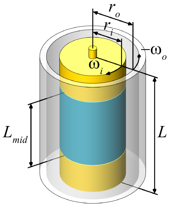
The core of our experimental set-up, the Taylor-Couette cell, is shown in figure 1. In the caption we give the respective length scales and their ratios. In particular, the fixed geometric dimensionless numbers are and . The details of the set-up are given in van Gils et al. (2011a). The working liquid is water at a continuously controlled constant temperature (precision K) in the range C - C. The accuracy in setting and maintaining a constant is based on direct angular velocity measurements of the T3C facility. To reduce edge effects, similarly as in Lathrop et al. (1992b, a), the torque is measured at the middle part (length ratio ) of the inner cylinder. Lathrop et al. (1992b)’s original motivation for this choice was that the height of the remaining upper and lower parts of the cylinder roughly equals the size of a pair of Taylor vortices. While the respective first or last Taylor vortex indeed will be affected by the upper and lower plates (which in our T3C cell are attached to the outer cylinder), the hope is that in the strongly turbulent regime the turbulent bulk is not affected by such edge effects. Note that for the laminar case (e.g. for pure outer cylinder rotation), this clearly is not the case, as has been known since Taylor (1923) – see, for example, the classical experiments by Coles & van Atta (1966), the numerical work by Hollerbach & Fournier (2004), or the review by Tagg (1994). For such weakly rotating systems, profile distortions from the plates propagate into the fluid and dominate the whole laminar velocity field. The velocity profile will then be very different from the classical height-independent laminar profile (see e.g. Landau & Lifshitz (1987)) with periodic boundary conditions in the vertical direction,
| (7) |
To control edge effects and ensure that they are indeed negligible in the strongly turbulent case under consideration here ( and , so well off the instability borders), we have measured time series of the angular velocity for various heights and radial positions with laser Doppler anemometry (LDA). We employ a backscatter LDA configuration set-up with a measurement volume of 0.07 mm x 0.07 mm x 0.3 mm. The seeding particles (PSP-5, Dantec Dynamics) have a mean radius of m and a density of g cm-3.
We estimate the minimum velocity difference between a particle and its surrounding fluid needed for the drag force to outweigh the centrifugal force . We put in m s-1 as a typical azimuthal velocity inside the TC gap at mid-gap radial position m, with g cm-3 as the density and kg m-1 s-1 as the dynamic viscosity of water at 21∘C. This results in m s-1, which is several orders of magnitude smaller than the typical velocity fluctuation inside the TC-gap of order m s-1, and hence centrifugal forces on the seeding particles are negligible.
We account for the refraction due to the cylindrical interfaces – details are given by Huisman et al. (2012b). Figure 2(a) shows the height dependence of the time-averaged angular velocity at mid-gap, , for and , corresponding to and . The dashed-dotted line at corresponds to the gap between the middle part of the inner cylinder, with which we measure the torque, and the upper part. Along the middle part the time-averaged angular velocity is independent within 1%, as is demonstrated in the inset, showing the enlarged relevant section of the axis. From the upper edge of the middle part of the inner cylinder towards the highest position that we can resolve, mm below the top plate, the mean angular velocity decays by only 5%. This finite difference might be due to the existence of Ekman layers near the top and bottom plate (Greenspan (1990)). Since at we have , as the upper plate is at rest for or , 95% of the edge effects on occur in such a thin fluid layer near the top (bottom) plate that we cannot even resolve it with our present LDA measurements.
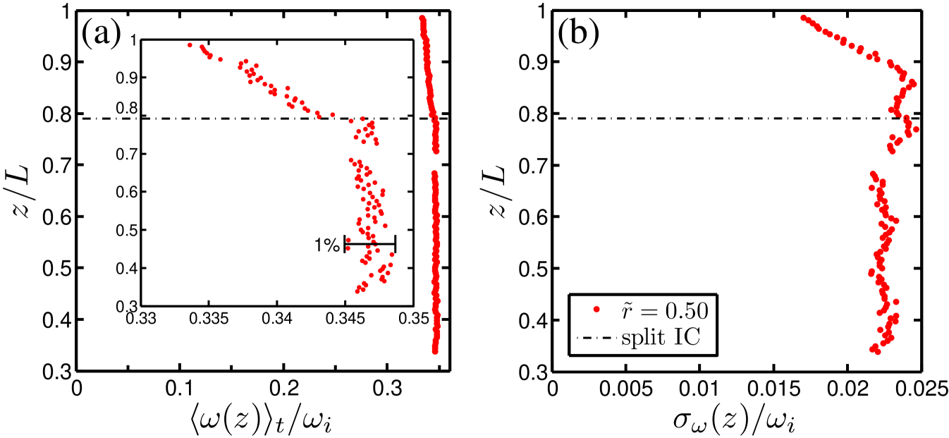
For the angular velocity fluctuations shown in figure 2(b), we observe a 25% decay in the upper 10% of the cylinder, but again in the measurement section of the inner cylinder there are no indications of any edge effects. The plots of figure 2 together confirm that edge effects are unlikely to play a visible role for our torque measurements in the middle part of the cylinder. Even the Taylor vortex roll structure, which dominates TC flow at low Reynolds numbers (Dominguez-Lerma et al. (1984, 1986); Andereck et al. (1986); Tagg (1994)), is not visible at all in the time-averaged angular velocity profile .
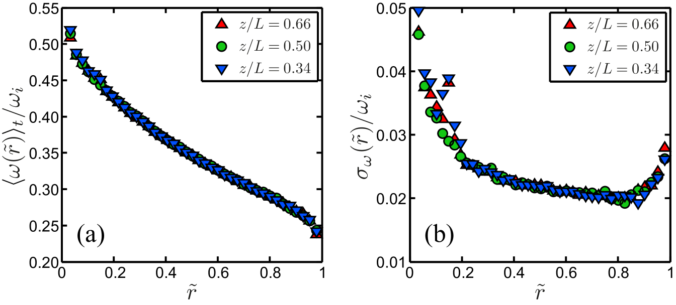
To double check that this independence holds not only at mid-gap but also for the whole radial profiles, we measured time series of at three different heights , and . The radial dependence of the mean value and of the fluctuations are shown in figure 3. The profiles are basically identical for the three heights, with the only exception of some small irregularity in the fluctuations at in the small region , whose origin is unclear to us. Note that in both panels of figure 3 the radial inner and outer boundary layers are again not resolved; in this paper we will focus on bulk properties and global scaling relations.
Based on the results of this section, we feel confident to claim that: (i) edge effects are unimportant for the global torque measurements done with the middle part of the inner cylinder reported in section 3; and (ii) the local profile and fluctuation measurements done close to mid-height , which will be shown and analysed in sections 4 and 5, are representative for any height in the middle part of the cylinder.
3 Global torque measurements
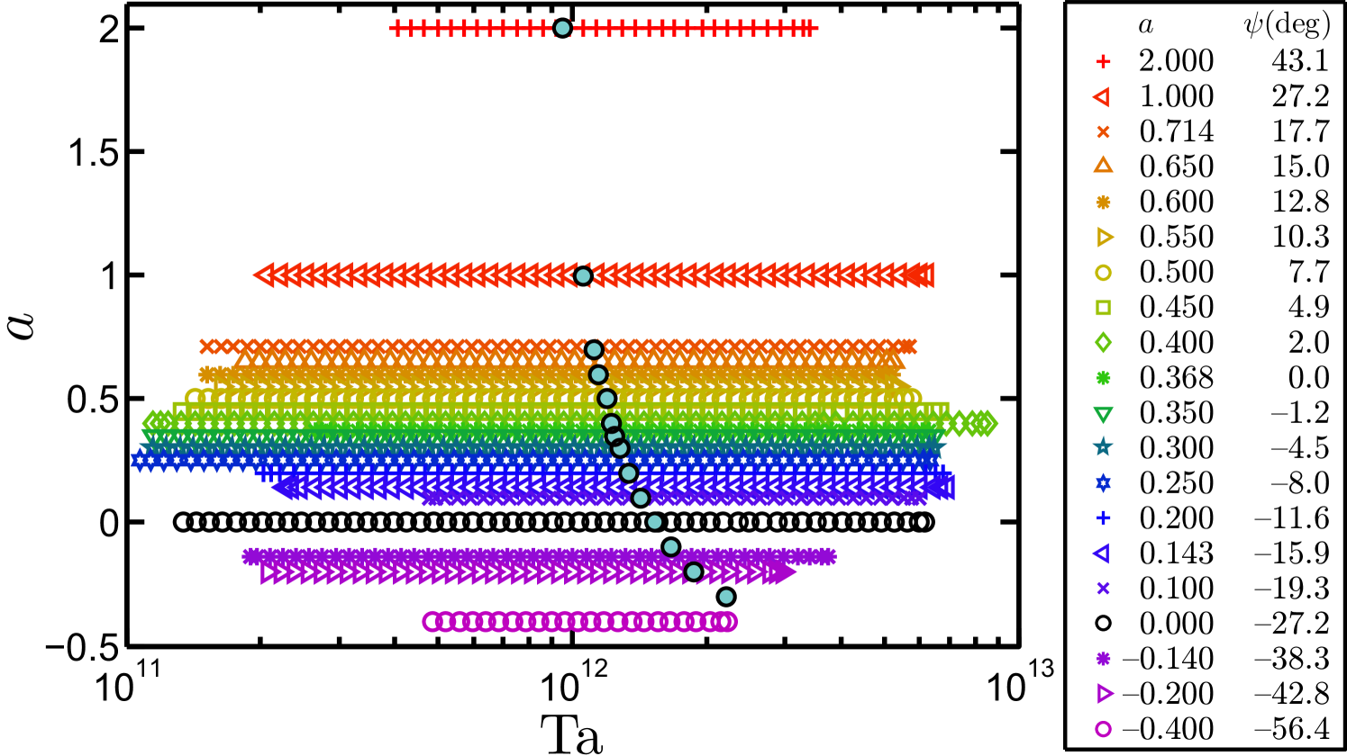
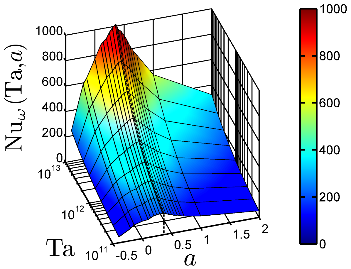
In this section we will present our data from the global torque measurements for independent inner and outer cylinder rotation, which complement and improve the precision of our earlier measurements in van Gils et al. (2011b). The data as functions of the respective pairs of control parameters () or (, ) for which we performed our measurements are given in tabular form in table 1 and in graphical form in figures 4(a) and 5.
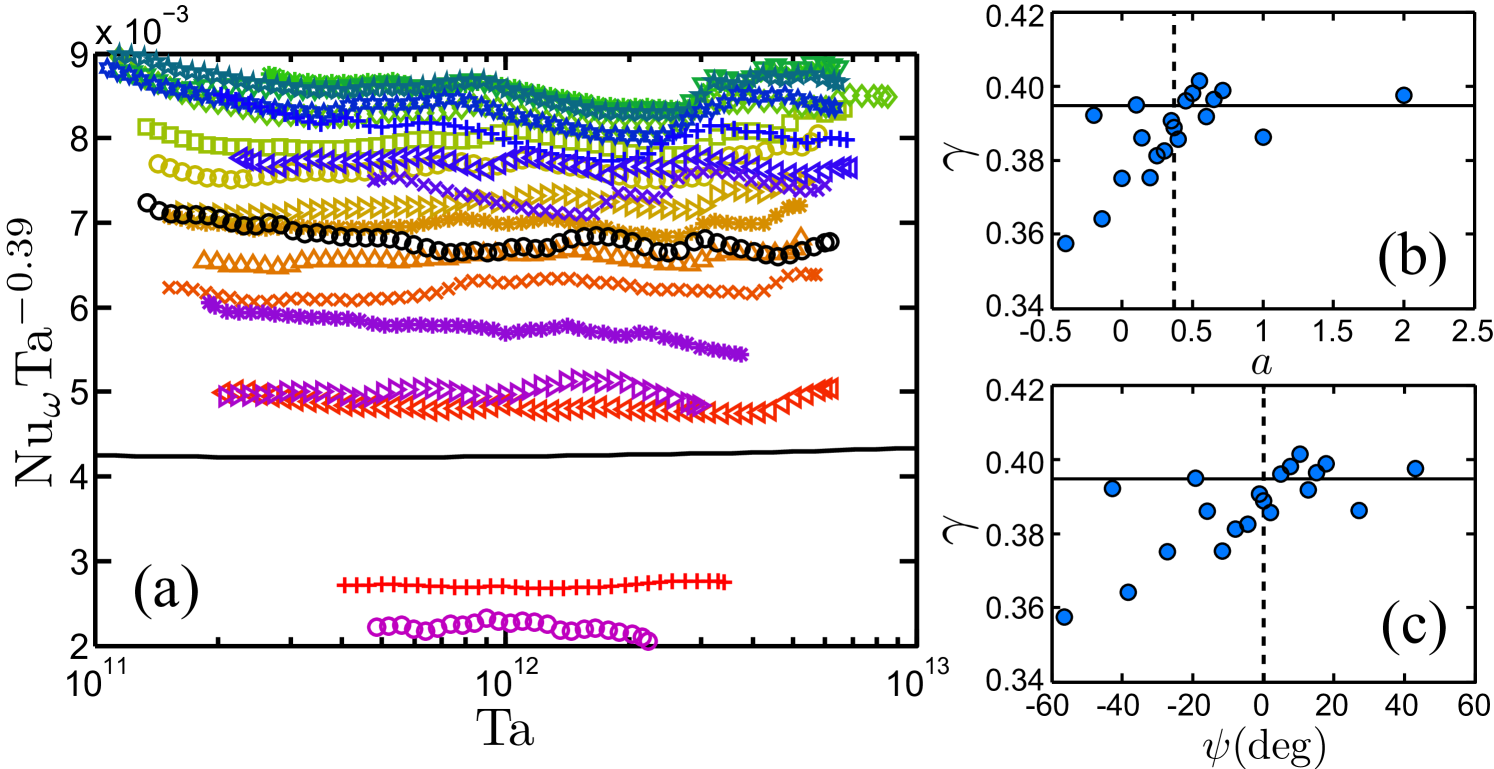
A three-dimensional overview of the found parameter dependences of the angular velocity transport is shown in figure 6. One immediately observes a pronounced maximum in with a considerable offset from the line . A more detailed view is obtained in cross-sections through figure 6 and in particular in compensated plots as shown in figure 7(a), where we divided by the approximate effective scaling . In this way we identify a universal effective scaling by averaging over the complete -range, ignoring -dependence and thus calling the scaling effective. If each curve for each is fitted individually, the resulting scaling exponents scatter with , but at most very slightly depend on ; see figure 7(b, c). For different linear fits below and above (actually below and above or , as will be introduced later on), we obtain for , the exponent slightly decreasing towards less counter-rotation, and a constant exponent for increasing counter-rotation beyond the optimum. The trend in the exponents for is small and compatible with a constant and a merely statistical scatter of . It is in this approximation that factorizes.
| min | max | min | max | min | max | min | max | min | max | min | max | min | max | ||||
|---|---|---|---|---|---|---|---|---|---|---|---|---|---|---|---|---|---|
| (deg.) | (rad s-1) | (rad s-1) | (rad s-1) | (rad s-1) | |||||||||||||
| 2.000 | 43.1 | 4.07 | 34.0 | 10.5 | 30.7 | -61.5 | -21.1 | 1.72 | 4.99 | -13.95 | -4.82 | 0.49 | 3.29 | 91 | 212 | 0.397 | 2.71 |
| 1.000 | 27.2 | 2.07 | 62.3 | 11.3 | 61.9 | -61.9 | -11.3 | 1.84 | 10.12 | -14.15 | -2.58 | 0.49 | 10.30 | 129 | 492 | 0.386 | 4.84 |
| 0.714 | 17.7 | 1.52 | 57.1 | 11.4 | 69.3 | -49.5 | -8.1 | 1.84 | 11.31 | -11.29 | -1.84 | 0.47 | 12.08 | 143 | 603 | 0.399 | 6.21 |
| 0.650 | 15.0 | 1.85 | 52.3 | 12.0 | 62.6 | -40.7 | -7.8 | 2.12 | 11.25 | -10.21 | -1.92 | 0.58 | 11.91 | 162 | 621 | 0.396 | 6.58 |
| 0.600 | 12.8 | 1.52 | 52.2 | 11.4 | 65.8 | -39.5 | -6.9 | 1.97 | 11.59 | -9.71 | -1.65 | 0.53 | 12.57 | 162 | 656 | 0.392 | 6.98 |
| 0.550 | 10.3 | 1.63 | 53.7 | 11.9 | 67.4 | -37.1 | -6.5 | 2.11 | 12.13 | -9.33 | -1.63 | 0.57 | 13.42 | 168 | 691 | 0.401 | 7.23 |
| 0.500 | 7.7 | 1.43 | 57.5 | 11.7 | 73.3 | -36.7 | -5.9 | 2.04 | 12.97 | -9.06 | -1.43 | 0.55 | 15.32 | 172 | 762 | 0.398 | 7.66 |
| 0.450 | 4.9 | 1.33 | 66.5 | 12.0 | 83.0 | -37.4 | -5.4 | 2.04 | 14.43 | -9.08 | -1.28 | 0.54 | 18.07 | 177 | 836 | 0.396 | 7.98 |
| 0.400 | 2.0 | 1.15 | 85.4 | 12.6 | 93.6 | -37.5 | -5.0 | 1.97 | 16.93 | -9.47 | -1.10 | 0.52 | 22.96 | 184 | 937 | 0.386 | 8.36 |
| 0.368 | 0.0 | 2.65 | 63.2 | 18.9 | 89.2 | -32.8 | -7.0 | 3.05 | 14.90 | -7.67 | -1.57 | 1.08 | 18.20 | 250 | 864 | 0.389 | 8.60 |
| 0.350 | -1.2 | 1.16 | 64.6 | 12.3 | 90.1 | -31.5 | -4.3 | 2.04 | 15.28 | -7.47 | -1.00 | 0.52 | 18.67 | 181 | 876 | 0.391 | 8.61 |
| 0.300 | -4.5 | 1.15 | 65.0 | 12.4 | 93.0 | -27.9 | -3.7 | 2.11 | 15.91 | -6.67 | -0.89 | 0.52 | 18.36 | 185 | 859 | 0.383 | 8.60 |
| 0.250 | -8.0 | 1.07 | 63.4 | 13.0 | 97.5 | -24.4 | -3.2 | 2.12 | 16.35 | -5.71 | -0.74 | 0.48 | 17.35 | 177 | 822 | 0.381 | 8.37 |
| 0.200 | -11.6 | 2.03 | 67.7 | 19.0 | 105.8 | -21.2 | -3.8 | 3.05 | 17.59 | -4.91 | -0.85 | 0.83 | 17.57 | 219 | 805 | 0.375 | 8.07 |
| 0.143 | -15.9 | 2.27 | 69.4 | 22.1 | 112.5 | -16.1 | -3.2 | 3.38 | 18.70 | -3.73 | -0.68 | 0.83 | 17.21 | 208 | 779 | 0.386 | 7.69 |
| 0.100 | -19.3 | 4.78 | 60.0 | 31.5 | 112.6 | -11.3 | -3.2 | 5.10 | 18.08 | -2.52 | -0.71 | 1.56 | 14.72 | 269 | 717 | 0.395 | 7.37 |
| 0.000 | -27.2 | 1.34 | 61.7 | 18.2 | 124.0 | 0.0 | 0.0 | 2.97 | 20.15 | 0.00 | 0.00 | 0.49 | 13.73 | 158 | 660 | 0.375 | 6.81 |
| -0.140 | -38.3 | 1.90 | 37.4 | 25.5 | 112.4 | 3.6 | 15.7 | 4.11 | 18.25 | 0.80 | 3.57 | 0.55 | 7.07 | 151 | 436 | 0.364 | 5.76 |
| -0.200 | -42.8 | 2.08 | 29.6 | 28.6 | 107.7 | 5.7 | 21.5 | 4.62 | 17.44 | 1.29 | 4.87 | 0.49 | 5.10 | 128 | 354 | 0.392 | 5.00 |
| -0.400 | -56.4 | 4.87 | 22.2 | 58.3 | 124.3 | 23.3 | 49.8 | 9.44 | 20.16 | 5.28 | 11.27 | 0.47 | 1.68 | 80 | 135 | 0.358 | 2.21 |
3.1 Ultimate regime
van Gils et al. (2011b) interpreted the effective scaling , similar to our currently obtained , as an indication of the so-called ‘ultimate regime’ – distinguished by both turbulent bulk and turbulent boundary layers. Such scaling was predicted by Grossmann & Lohse (2011) for very strongly driven RB flow. As detailed in Grossmann & Lohse (2011), it emerges from a scaling with logarithmic corrections originating from the turbulent boundary layers. Remarkably, the corresponding wind Reynolds number scaling in RB flow does not have logarithmic corrections, i.e. . These RB scaling laws for the thermal Nusselt number and the corresponding wind Reynolds number have been confirmed experimentally by Ahlers et al. (2011) for and by He et al. (2012) for . According to the EGL theory this should have its correspondence in TC flow. That leads to the interpretation of as an indication for the ultimate state in the presently considered TC flow. Furthermore, Huisman et al. (2012a) indeed also found from particle image velocimetry (PIV) measurements in the present strongly driven TC system the predicted (Grossmann & Lohse, 2011) scaling of the wind, .
We note that in our available regime the effective scaling law is practically indistinguishable from the prediction of Grossmann & Lohse (2011), namely,
| (8) |
with the logarithmic corrections detailed in equations (7) and (9) of Grossmann & Lohse (2011). The result from (8) is shown as a solid line in figure 7(a), showing the compensated plot . Indeed, only detailed inspection reveals that the theoretical line is not exactly horizontal.
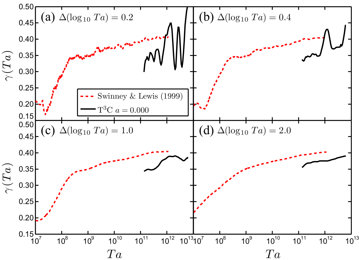
Thus, strictly speaking, there is a dependence of the scaling exponent , as was clearly evidenced by Lathrop et al. (1992a) and Lewis & Swinney (1999) in a much larger range. In figure 8 we present our local for the case of and we compare it to the data from Lewis & Swinney (1999). Similar to Lewis & Swinney (1999) we calculate ) by using a sliding least-squares linear fit over a certain range, as indicated by the top left corner of panels (a–d). The narrow averaging range used in figure 8(a) results into a strongly fluctuating . The origin of these fluctuations may be different turbulent flow states (e.g. different number of Taylor vortices); future studies should shed more light onto this. When averaging over a wider range, our data recover a monotonically increasing trend, as can be seen in figure 8(d), which is in line with Lathrop et al. (1992a) and Lewis & Swinney (1999). Clearly, with their large- measurements, these authors also already were in the ultimate TC regime.
This gives rise to the following question: Where does the ultimate turbulence regime set in for turbulent TC flow? To find out, we calculate the shear Reynolds number , where is the thickness of the kinetic boundary layer, still being of Prandtl type, and is the shear velocity across . The latter we estimate as . Correspondingly, we estimate the kinetic Prandtl-Blasius type BL thickness as (see e.g. Landau & Lifshitz (1987)), with set to . This results in a shear Reynolds number of . For the wind Reynolds number we take our experimental result based on PIV measurements (Huisman et al. (2012a)), namely (in the regime from to , for ). This implies that the relative contribution of the wind is only around in this regime. Nonetheless, we take it into consideration in figure 9(a), in which we plot versus , retrieving the effective scaling . That figure also shows the result of Ostilla et al. (2012) from direct numerical simulation (DNS), who found in the regime from to . Again, also here the relative contribution of the wind is very small, namely around . These numerical results give an effective scaling of , very similar to our experimental findings, even prefactor-wise.
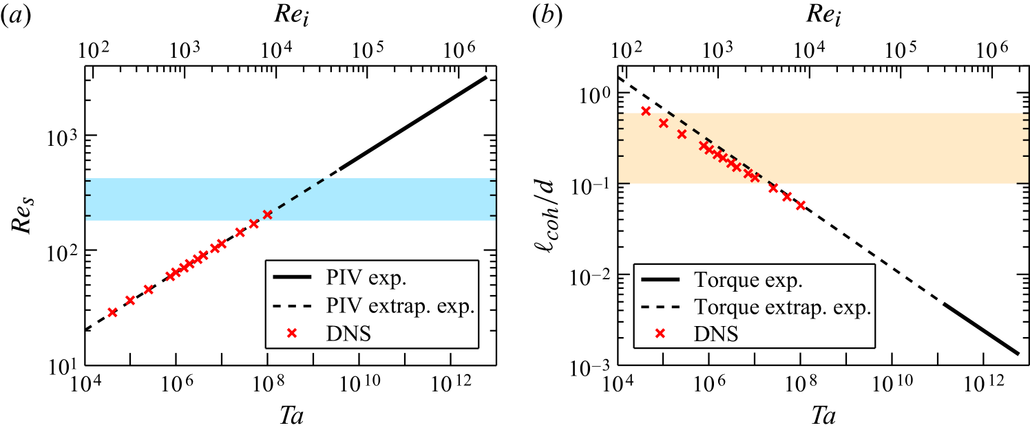
The Prandtl-Blasius type BL becomes turbulent for a shear Reynolds number larger than a critical shear Reynolds number or transition shear Reynolds number , which is known to be in the range between 180 and 420 (see e.g. Landau & Lifshitz (1987)). This range is shown as shaded in figure 9: all of our experimental data points of this present paper (solid line) are beyond that onset. So, indeed, we are in the ultimate regime. In contrast, the numerical data points by Ostilla et al. (2012) are in the Prandtl-Blasius regime with laminar-type boundary layers.
The transition between these two regimes occurs in between. The range 180–420 for the transitional shear Reynolds number here (i.e., for the present and ) corresponds to a range between and for the transitional Taylor number and to a range between and for the transitional (inner) Reynolds number . This corresponds to the transitional Reynolds number found by Lewis & Swinney (1999), see their figure 3, in which the transition to the ultimate regime is identified at a Reynolds number . Below that value Lewis & Swinney (1999) find a very steep increase of the local slope with ; beyond the transition the increase is much less. (Here we have translated Lewis & Swinney (1999)’s finding into the notation of this present paper.) We stress again that the values given in this and the next subsection hold for . How the values of the transitional Reynolds or Taylor number depend on remains an important question for future research.
Both in our experiment and in the experiments by Lewis & Swinney (1999) the logarithmic corrections in (8) are visible and have the consequence that the “real” ultimate scaling is never achieved. As explained in Grossmann & Lohse (2011) – and, differently and with a different result, much earlier in Kraichnan (1962)) – these logarithmic corrections are a consequence of the logarithmic velocity profile in the turbulent boundary layers. Only by destroying these logarithmic profiles by extreme wall roughness as done in TC experiments by van den Berg et al. (2003) or in RB experiments by Roche et al. (2001) or by replacing the walls by periodic boundary conditions (and a volume forcing) as done in numerical simulations by Lohse & Toschi (2003); Calzavarini et al. (2005); Schmidt et al. (2012) can one recover the 1/2 scaling exponent, which is obtained in the strict upper-bound of Doering & Constantin (1994).
3.2 Comparison Taylor-Couette turbulence with Rayleigh-Bénard turbulence
To get an idea of the extension of the non-ultimate turbulence regime in TC flow, we also estimate the coherence length , below which the spatial coherence of structures in the flow becomes small enough to allow for developed turbulence in the flow. Typically, one estimates the coherence length as a multiple of the (mean) Kolmogorov length scale , namely . The factor of 10 between these two length scales is motivated by the transition between viscous subrange and inertial subrange, which is known to happen at a scale around (see e.g. Effinger & Grossmann (1987)). Here is the mean energy dissipation rate. That can be obtained from the angular velocity flux (see (4.7) of EGL), namely
| (9) |
reflecting the statistical balance between external driving and internal dissipation. As pointed out in EGL, a more elegant way to write this balance is
| (10) |
In any case, we can use our data for to calculate the mean Kolmogorov length scale and thus the coherence length . In figure 9(b) we show as a function of or (for and ). When the coherence length becomes smaller than, say, 0.1–0.5 times the outer length scale , one can reasonably start to speak of a developed turbulence regime in the bulk in between the inner scale and the outer scale . According to figure 9(b), this onset of a developed turbulence regime in the bulk, but still with Prandtl-Blasius type boundary layers (see Sun et al. (2008); Zhou et al. (2010)), occurs at Taylor numbers between and or onset (inner) Reynolds numbers between 300 and 3000, far below the regime of our present experiments, but in the regime of the numerical simulations of Ostilla et al. (2012). The corresponding numbers for smaller coherence in RB flow are given in figure 1 of Sugiyama et al. (2007). For , a developed turbulence regime in the bulk becomes possible beyond .
| TC | RB | |
|---|---|---|
| Loss of spatial coherence | ||
| (defined via ) | ||
| BL shear instability | ||
| (defined via ) |
Figure 9(a, b) reveals that there should be a TC flow range with Prandtl-Blasius type (laminar) BLs and a turbulent bulk roughly in between and or in between and . This regime was explored in the earlier experiments by Lathrop et al. (1992b, a); Lewis & Swinney (1999) and others – it cannot be accessed with water as operating liquid in our T3C set-up as the angular velocities would have to be too low for reasonable precision. We could, however, explore that regime with more viscous liquids also with our T3C set-up.
Our present estimates for TC flow and the earlier findings and estimates for RB flow are summarized in table 2. The table gives rise to the interesting question: Why is the “classical regime” (as it is called by Ahlers) in between and , in which a laminar-type BL and a turbulent bulk coexist and in which the unifying theory of Grossmann & Lohse (2000, 2001, 2002, 2004) is applicable, so extended in RB turbulence, but so small in TC turbulence? Or, in other words: Why does the ultimate regime with its turbulent BLs set in for much smaller in TC flow as compared to the extremely high values for that onset in RB flow?
We think that the answer lies in the much higher efficiency of the shear driving in TC flow as compared to the thermal driving in RB flow. In RB flow the shear instability of the kinetic BL is induced by the thermal driving only indirectly; namely, the driving first induces a large scale wind, which then in turn builds up the shear near the boundaries. In TC flow the flow is directly driven by the rotating inner cylinder, giving rise to a very large direct shear. As pointed out above, the large scale wind with its strength only means a small correction of to in the calculation of the shear Reynolds number. As roughly , a factor of 20 in the shear Reynolds number leads to the huge difference in the typical onset Taylor number.
3.3 Optimal angular velocity transport
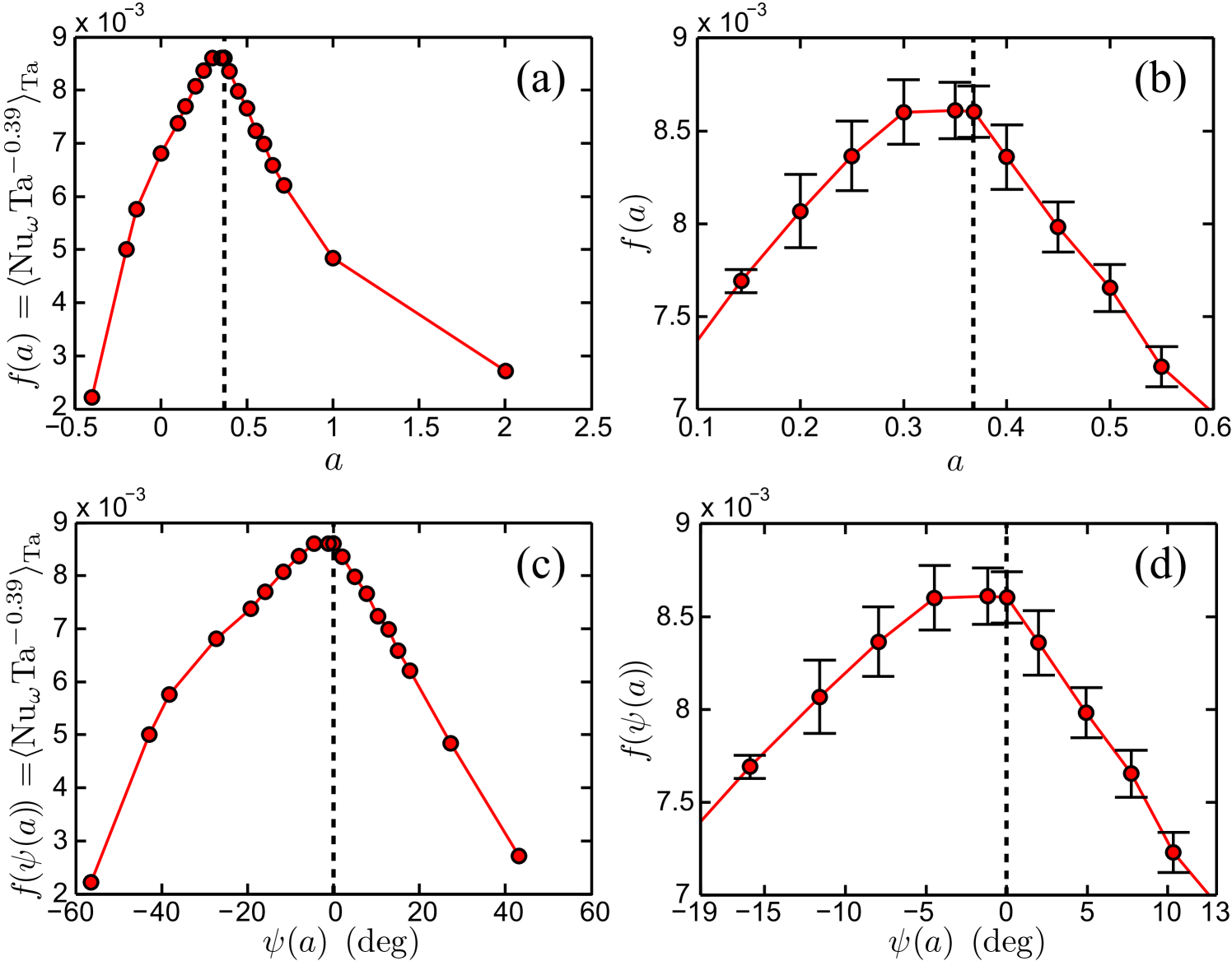
Coming back to our experimental data on TC: the (nearly) horizontal lines in figure 7(a) imply that within the present experimental precision nearly factorizes in . We now focus on the dependence of the angular velocity flux amplitude , shown in figure 10(a, b), and its interpretation. One observes a very pronounced maximum at , reflecting the optimal angular velocity transport from the inner to the outer cylinder at that angular velocity ratio. This value is obtained by averaging over the three data points making up the small plateau visible in figure 10(b). Naively, one might have expected that has its maximum at , i.e. (no outer cylinder rotation) since outer cylinder rotation stabilizes an increasing part of the flow volume for increasing counter-rotation rate. On the other hand, outer cylinder rotation also enhances the total shear of the flow, leading to enhanced turbulence, and thus more angular velocity transport is expected. The dependence of thus reflects the mutual importance of both these effects.
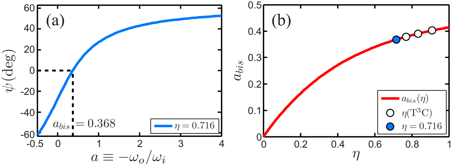
Generally, one expects an increase of the turbulent transport if one goes deeper into the control parameter range () in which the flow is unstable. We speculate that the optimum positions for the angular velocity transport should consist of all points in parameter space that are equally distant from both the right branch (first quadrant, co-rotation) of the instability border and its left branch (second quadrant, counter-rotation). In the inviscid approximation (), these two branches are given by the Rayleigh criterion, , resulting in the lines given by the relations and , which translate into and , respectively. The line of equal distance from both is the angle bisector of the instability range. Its relation can easily be calculated to be
| (11) |
For this gives . Noteworthily, the measured value agrees indistinguishably within experimental precision with the bisector line, supporting our interpretation. It also explains why only the lines const scan the parameter space properly. This reflects the straight character of the linear instability lines – as long as one is not too close to them to see the details of the viscous corrections, i.e. if is large and is well off the instability borders at for co-rotation and for counter-rotation.
Instead of characterizing the lines by the slope parameter , one can introduce the angle between the line of chosen and the angle bisector of the instability range denoted by ; thus corresponds to :
| (12) |
The transformation (12) is shown in figure 11(a) and the resulting in figure 10(c). The function as a function of is strongly asymmetric both around its peak at and at its tails, presumably because of the different viscous corrections at (decreasing towards the inviscid Rayleigh line) and at (non-vanishing, even increasing correction , and non-normal nonlinear (shear) instability (see e.g. Grossmann (2000))).
We do not yet know whether the optimum of coincides with the bisector of the Rayleigh-unstable domain for all . Both could coincide incidentally for , analysed here. But if this were the case for all , we can predict the dependence of . This, then, is given by (11). This function is plotted in figure 11. In future experiments we shall test this dependence with our T3C facility. The three extra points we will be able to achieve are marked as white, empty circles. The precision of our facility is good enough to test (11), but clearly further experiments at much smaller are also needed.
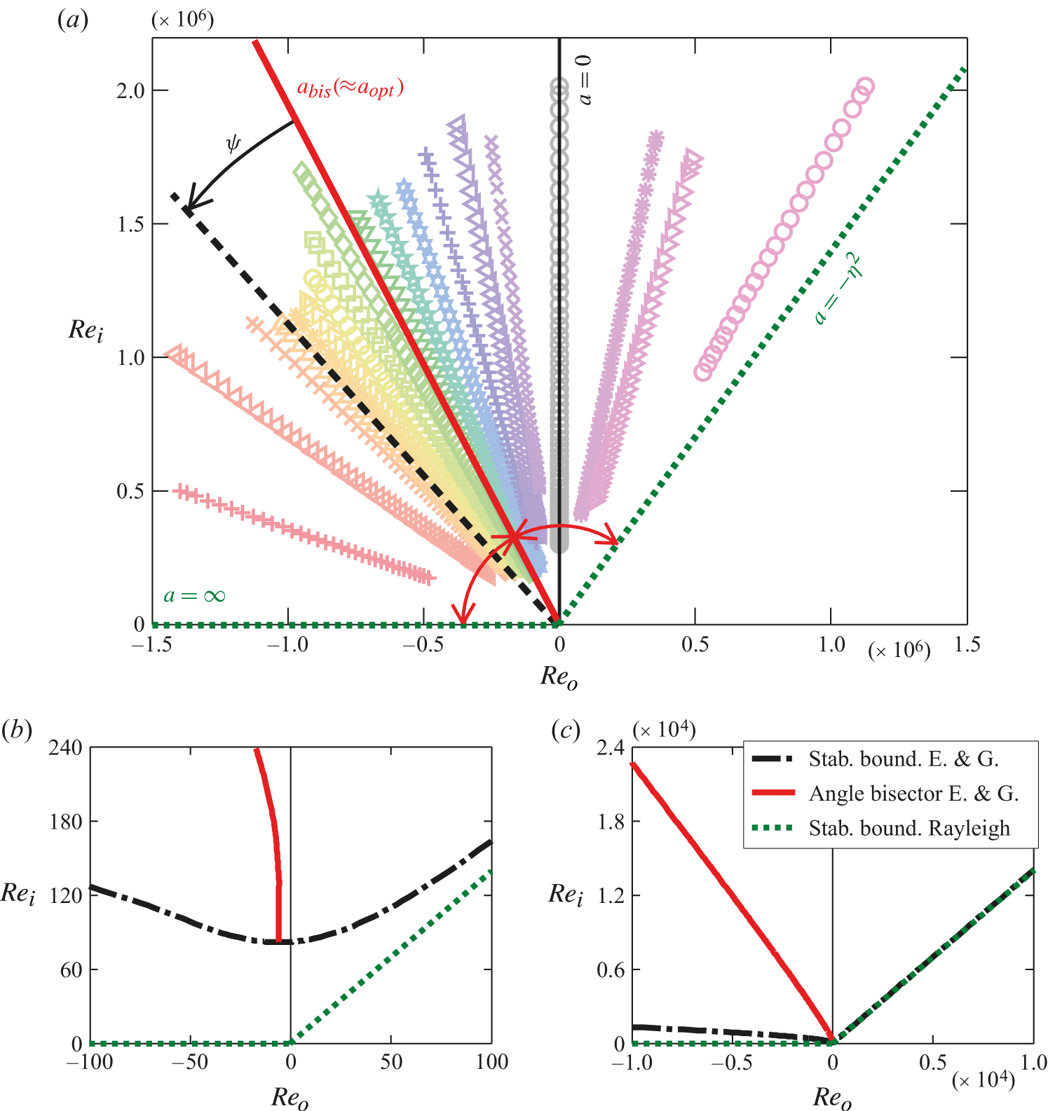
We note that, for smaller , one can no longer approximate the instability border by the inviscid Rayleigh lines. The effect of viscosity on the shape of the border lines has to be taken into account. The angle bisector of the instability range in (, ) parameter space (figure 4(a)) will then deviate from a straight line; we therefore also expect this for . The viscous corrections of the Rayleigh instability criterion were first numerically calculated by Dominguez-Lerma et al. (1984) for the case of , and then analytically estimated by Esser & Grossmann (1996) and later fitted by Dutcher & Muller (2007). Figure 4(b, c) shows enlargements of the (, ) parameter space, together with the Rayleigh criterion (dotted green lines) and the Esser & Grossmann (1996) analytical curve (dashed-dotted black) for . Note that the minimum of that curve is not at , but shifted to a slightly negative value , where the instability sets in at . If we again assume that the optimum position for turbulent transport is distinguished by equal distance to the two branches of the Esser-Grossmann curve, we obtain the red curve in figure 4(b). On the scale of figure 4(a, c) it is indistinguishable from a straight line through the origin and can hence be described by (11). As another consequence of the viscous corrections, the factorization of the angular velocity transport flux will no longer be a valid approximation in the parameter regime shown in figure 4(b). For this to hold, must be large and well off the instability lines. This could be tested further by choosing the parameter sufficiently large, the line approaching or even cutting the stability border for strong counter-rotation. Then the factorization property will clearly be lost.
Future low- experiments and/or numerical simulations for various will show how well these ideas on understanding the existence and value of , being near or equal to , are correct or deserve modification. Of course, there will be some deviations due to the coherent structures in the flow at lower , due to the influence of the number of rolls, etc. Similarly to how in RB the scaling shows discontinuities, the TC scaling exponent of shows all these structures for insufficiently large – see figure 3 of Lewis & Swinney (1999), for example, in which one sees how strongly the exponent depends on up to ( about up to ).
4 Local LDA angular velocity radial profiles
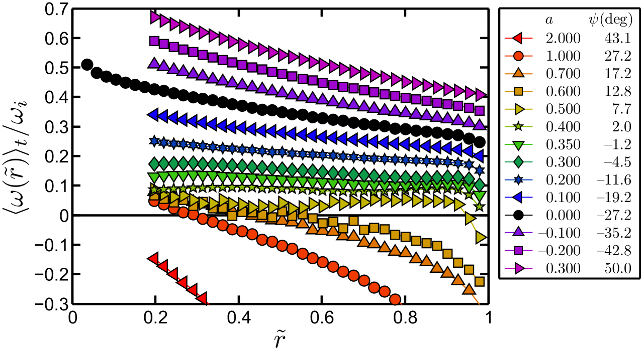
We now wonder whether the distinguishing property of the flow at (maximal angular velocity transport) is also reflected in other flow characteristics. We therefore performed LDA measurements of the angular velocity profiles in the bulk, close to mid-height, , at various : see table 3 for a list of all measurements, figure 12 for the mean profiles at fixed height , and figure 13 for the rescaled profiles , also at fixed height . With our present LDA technique, we can only resolve the velocity in the radial range ; there is no proper resolution in the inner and outer boundary layers. Because the flow close to the inner boundary region requires substantially more time to be probed with LDA, due to disturbing reflections of the measurement volume on the reflecting inner cylinder wall necessitating the use of more stringent Doppler burst criteria, we limit ourselves to the range .
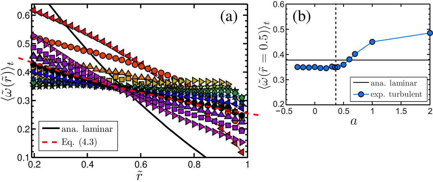
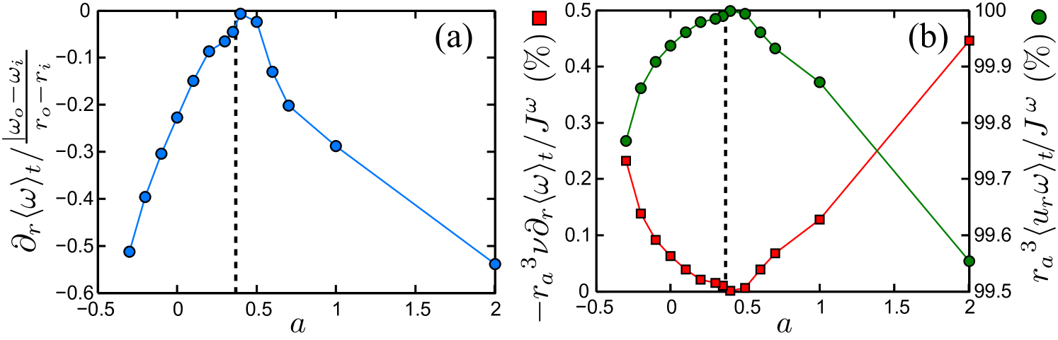
From figure 12 it is seen that for nearly all co- and counter-rotating cases the slope of is negative. Only around do we find a zero mean angular velocity gradient in the bulk. This case is very close to and . The normalized angular velocity gradient as a function of is shown in figure 14(a). Indeed, it has a pronounced maximum and zero mean angular velocity gradient very close to , the position of optimal angular velocity transfer. van Hout & Katz (2011), who performed PIV measurements of TC flow in air around , report a similar trend of a diminishing angular velocity gradient in the center of the TC gap for their investigated coming from down towards , i.e. well in the counter-rotating regime. We speculate that their trend would continue and result in a diminishing slope of angular velocity when decreasing further to their (unreported) case of . Interestingly, the result of a zero angular velocity gradient across the gap is quite similar to what can be found in Taylor vortex flow, for which the axially averaged circumferential momentum or velocity is nearly uniform across the gap in the bulk (see e.g. Marcus (1984); Werne (1994)). We note that in strongly turbulent RB flow the temperature also has a (practically) zero mean gradient in the bulk – see, for example, the recent review by Ahlers et al. (2009).
A transition of the flow structure at can also be confirmed in figure 13(a), in which we have rescaled the mean angular velocity at fixed height as
| (13) |
We observe that up to the curves for for all go through the mid-gap point , implying the mid-gap value for the time-averaged angular velocity. However, for , i.e. stronger counter-rotation, the angular velocity at mid-gap becomes larger, as seen in figure 13(b).
Figure 14(b) shows the relative contributions of the molecular and the turbulent transport to the total angular velocity flux (6), i.e. for both the diffusive and the advective term. The latter always dominates by far with values beyond 99%, but at the advective term contributes 100% to the angular velocity flux and the diffusive term nothing, corresponding to the zero mean angular velocity gradient in the bulk at that . This special situation perfectly resembles RB turbulence for which, due to the absence of a mean temperature gradient in the bulk, the whole heat transport is conveyed by the convective term. In the (here unresolved) kinetic boundary layers the contributions just reverse: The convective term strongly decreases if approaches the cylinder walls at 0 or 1 since ( in RB), while the diffusive term (heat flux in RB) takes over at the same rate, as the total flux is an -independent constant.
| (deg.) | (rad s-1) | (rad s-1) | (s-1) | (s-1) | ||||||
|---|---|---|---|---|---|---|---|---|---|---|
| 2.000 | 43.1 | 0.95 | 16.3 | -32.6 | 0.26 | -0.74 | 35 | 60 | 70 | 2.4 |
| 1.000 | 27.2 | 1.06 | 25.8 | -25.8 | 0.42 | -0.58 | 26 | 60 | 52 | 1.6 |
| 0.700 | 17.2 | 1.12 | 31.2 | -21.9 | 0.51 | -0.49 | 55 | 80 | 46 | 0.7 |
| 0.600 | 12.8 | 1.15 | 33.6 | -20.1 | 0.54 | -0.46 | 67 | 80 | 56 | 0.5 |
| 0.500 | 7.7 | 1.20 | 36.4 | -18.2 | 0.59 | -0.41 | 31 | 60 | 63 | 0.6 |
| 0.400 | 2.0 | 1.22 | 39.5 | -15.8 | 0.64 | -0.36 | 10 | 25 | 57 | 0.7 |
| 0.350 | -1.2 | 1.25 | 41.4 | -14.5 | 0.67 | -0.33 | 11 | 25 | 45 | 0.5 |
| 0.300 | -4.5 | 1.28 | 43.6 | -13.1 | 0.70 | -0.30 | 12 | 25 | 64 | 0.8 |
| 0.200 | -11.6 | 1.34 | 48.3 | -9.65 | 0.78 | -0.22 | 14 | 25 | 78 | 1.0 |
| 0.100 | -19.2 | 1.42 | 54.2 | -5.46 | 0.88 | -0.12 | 17 | 25 | 93 | 1.3 |
| 0.000 | -27.2 | 1.53 | 61.8 | 0.00 | 1.00 | 0.00 | 13 | 25 | 72 | 2.3 |
| -0.100 | -35.2 | 1.67 | 71.9 | 7.21 | 1.16 | 0.16 | 25 | 25 | 147 | 1.7 |
| -0.200 | -42.8 | 1.87 | 85.7 | 17.1 | 1.39 | 0.39 | 22 | 25 | 121 | 1.6 |
| -0.300 | -50.0 | 2.21 | 106.0 | 31.9 | 1.72 | 0.72 | 6 | 25 | 32 | 7.5 |
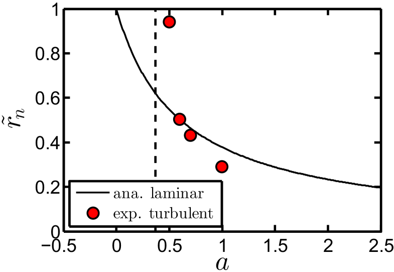
From the measurements presented in figure 12, we can extract the neutral line , defined by at fixed height for the turbulent case. The neutral line is, of course, part of a neutral surface throughout the TC volume. We expect that, for large , the flow will be so much stabilized that an axial dependence of the location of the neutral line shows up, in spite of the large numbers, in contrast to the cases where we expect the location of the neutral line to be axially independent for large enough . The results for are shown in figure 15. Note that, while for (co-rotation) there obviously is no neutral line at which , for a neutral line exists at some position . As long as it is still within the outer kinematic BL, we cannot resolve it. This turns out to be the case for . But for the neutral line can be observed within the bulk and is well resolved with our measurements. So, again, we see two regimes: for in the laminar case the stabilizing outer cylinder rotation shifts the neutral line inwards, but, due to the now free boundary between the stable outer range and the unstable range between the neutral line and the inner cylinder, the flow structures extend beyond . Thus also in the turbulent flow case the unstable range flow extends to the close vicinity of the outer cylinder. The increased shear and the strong turbulence activity originating from the inner cylinder rotation are too strong and prevent the neutral line being shifted off the outer kinematic BL. As described in Esser & Grossmann (1996), this is the very mechanism that shifts the minimum of the viscous instability curve to the left of the axis. Therefore, the observed behaviour of the neutral line position as a function of is another confirmation of the above idea that coincides with the angle bisector of the instability range in parameter space. The small- and the large- behaviours perfectly merge. Only for is the stabilizing effect from the outer cylinder rotation strong enough, and the width of the stabilized range broad enough, so that a neutral line can be detected in the bulk of the TC flow. This behaviour is similar to what is reported by van Hout & Katz (2011), see their figure 6.
One would expect that for much weaker turbulence , the capacity of the turbulence around the inner cylinder to push the neutral line outwards would decrease, leading to a smaller for these smaller Taylor numbers. Numerical simulations by H. Brauckmann and B. Eckhardt of the University of Marburg ( up to ) and independently ongoing DNS by Ostilla et al. (2012) of the University of Twente (presently up to ) seem to confirm this view.
For much weaker turbulence, one would also expect a more pronounced height dependence of the neutral line, which will be pushed outwards where the Taylor rolls are going outwards and inwards where they are going inwards. Based on our height dependence studies of section 2, we expect that this height dependence will be much weaker or even fully washed out in the strongly turbulent regime in which we operate the TC apparatus. However, in figure 15 we observe that the neutral line in the turbulent case lies more inside than in the laminar case, and this result is difficult to rationalize apart from assuming some axial dependence of the neutral line location, i.e. more outwards locations of the neutral line at larger and smaller height. In future work we will study the axial dependence of the neutral line in the turbulent and counter-rotating case in more detail.
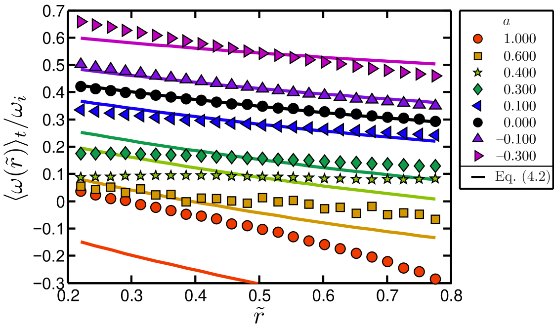
For completeness, we also compare our experimental angular velocity profiles with those employed in the upper-bound theory by Busse (1972). Busse (1972) derived an expression for the angular velocity profiles in the limit of infinite Reynolds number. Translating that expression to the notation used in the present work gives
| (14) |
As already shown by Lewis & Swinney (1999), for the case excellent agreement between the Busse profile and the experimental one is found. However, for farther away from zero, there is a greater discrepancy between the experimental data and the profiles suggested by the upper-bound theory, as shown in figure 16(a). When we rescale the angular velocity profiles to , according to (13), the profiles as given by the upper-bound theory (Busse, 1972) fall on top of each other for all ,
| (15) |
In contrast to the collapsing upper-bound profiles, the experimental data in figure 16(b) show a different trend. Clearly, the profiles suggested by the upper bound theory are in general not a good description of the physically realized profiles, apart from the case. Given the complexity of the flow, this may not be surprising.
While in this section we have only focused on the time-mean values of the angular velocity, in the following section we will give more details on the probability density functions (p.d.f.) in the two different regimes below and above and thus on the different dynamics of the flow in these two different regimes.
5 Turbulent flow organization in the gap between the cylinders
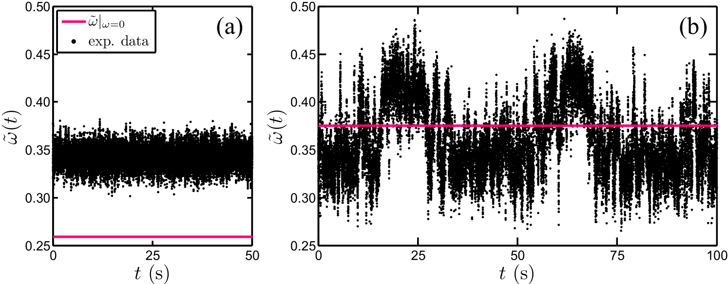
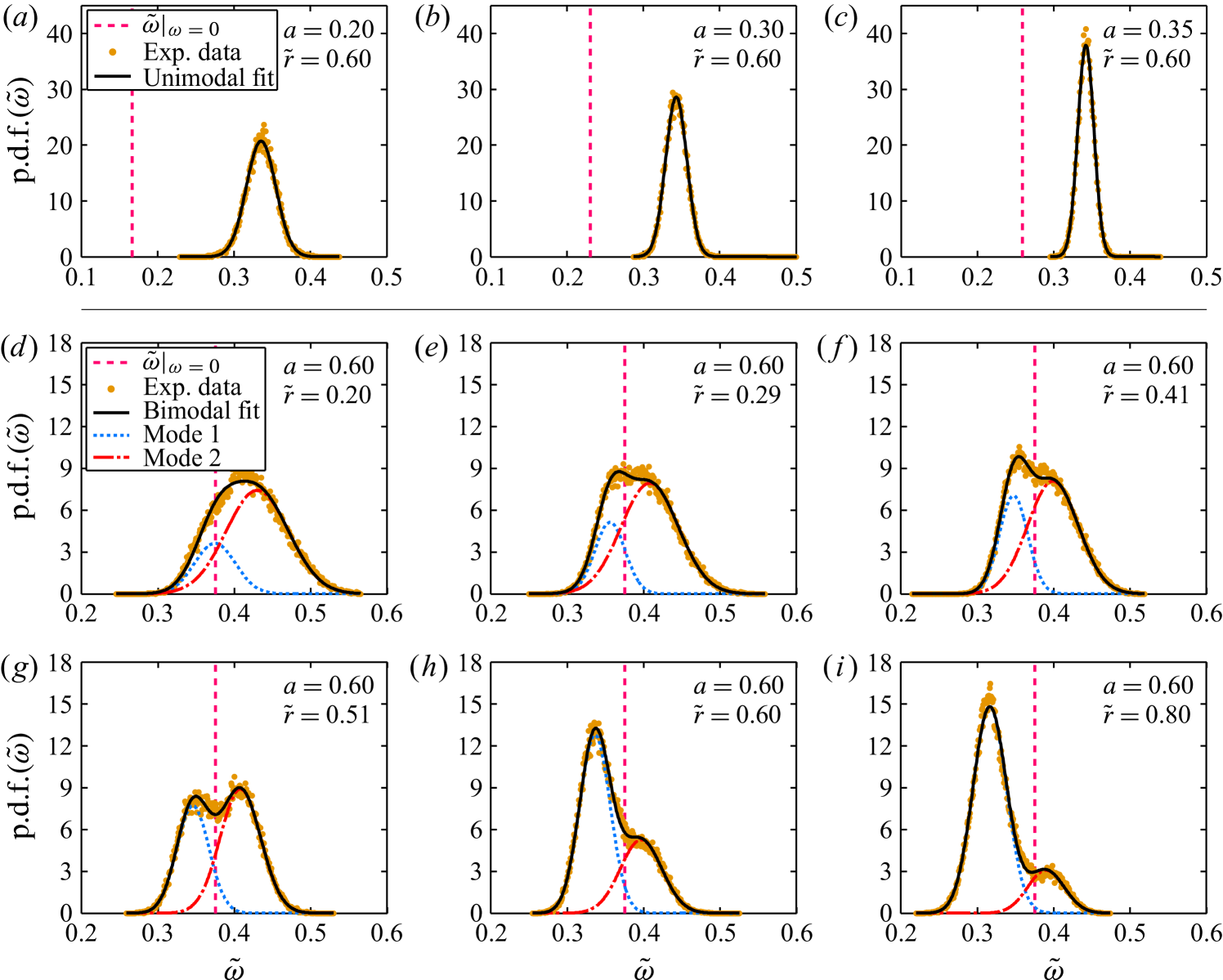
Time series of the angular velocity at below the optimum amplitude at (co-rotation dominates) and above the optimum at (counter-rotation dominates) are shown in figure 17(a, b), respectively. While in the former case we always have and a Gaussian distribution (see figure 18a), in the latter case we find a bimodal distribution with one mode fluctuating around a positive angular velocity and one mode fluctuating around a negative angular velocity. This bimodal distribution of is confirmed in various p.d.f.s shown in figure 18. We interpret this intermittent behaviour of the time series as an indication of turbulent bursts originating from the turbulent region in the vicinity of the inner cylinder and penetrating into the stabilized region near the outer cylinder. We find such bimodal behaviour for all (see figure 18d–i), whereas for we find a unimodal behaviour (see figure 18a–c). Apart from one case () we do not find any long-time periodicity of the bursts in . In future work we will perform a full spectral analysis of long time series of for various and .
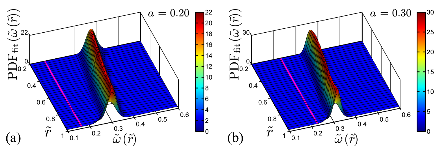
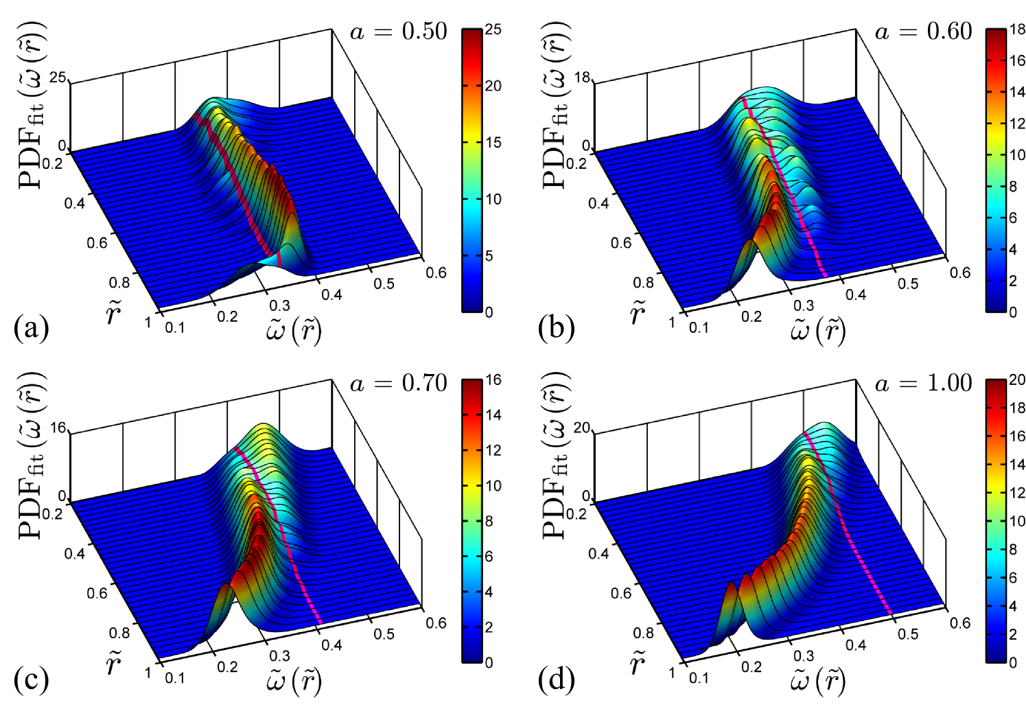
Three-dimensional visualizations of the p.d.f. for all are provided in figure 19 for unimodal cases and in figure 20 for bimodal cases . In the latter figure the switching of the system between positive and negative angular velocity becomes visible.
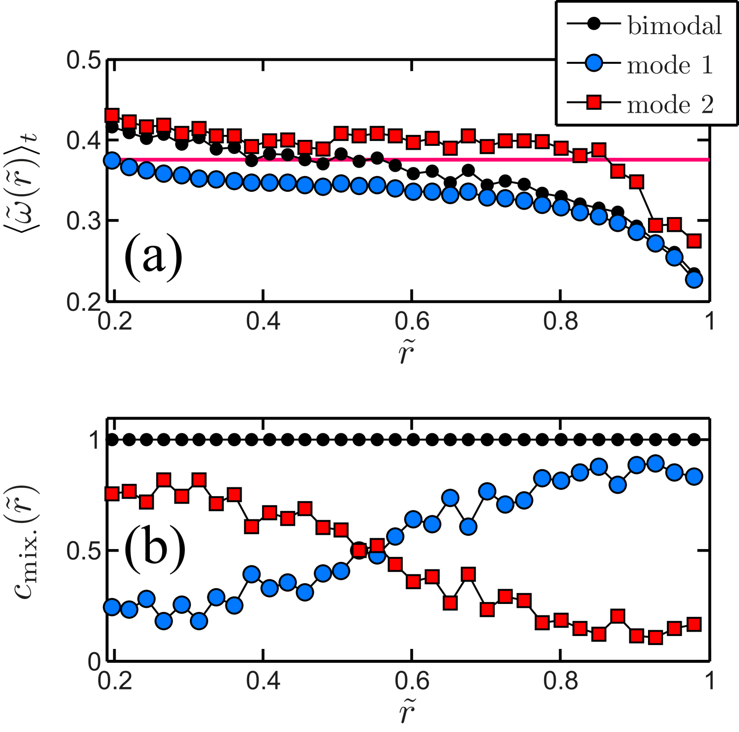
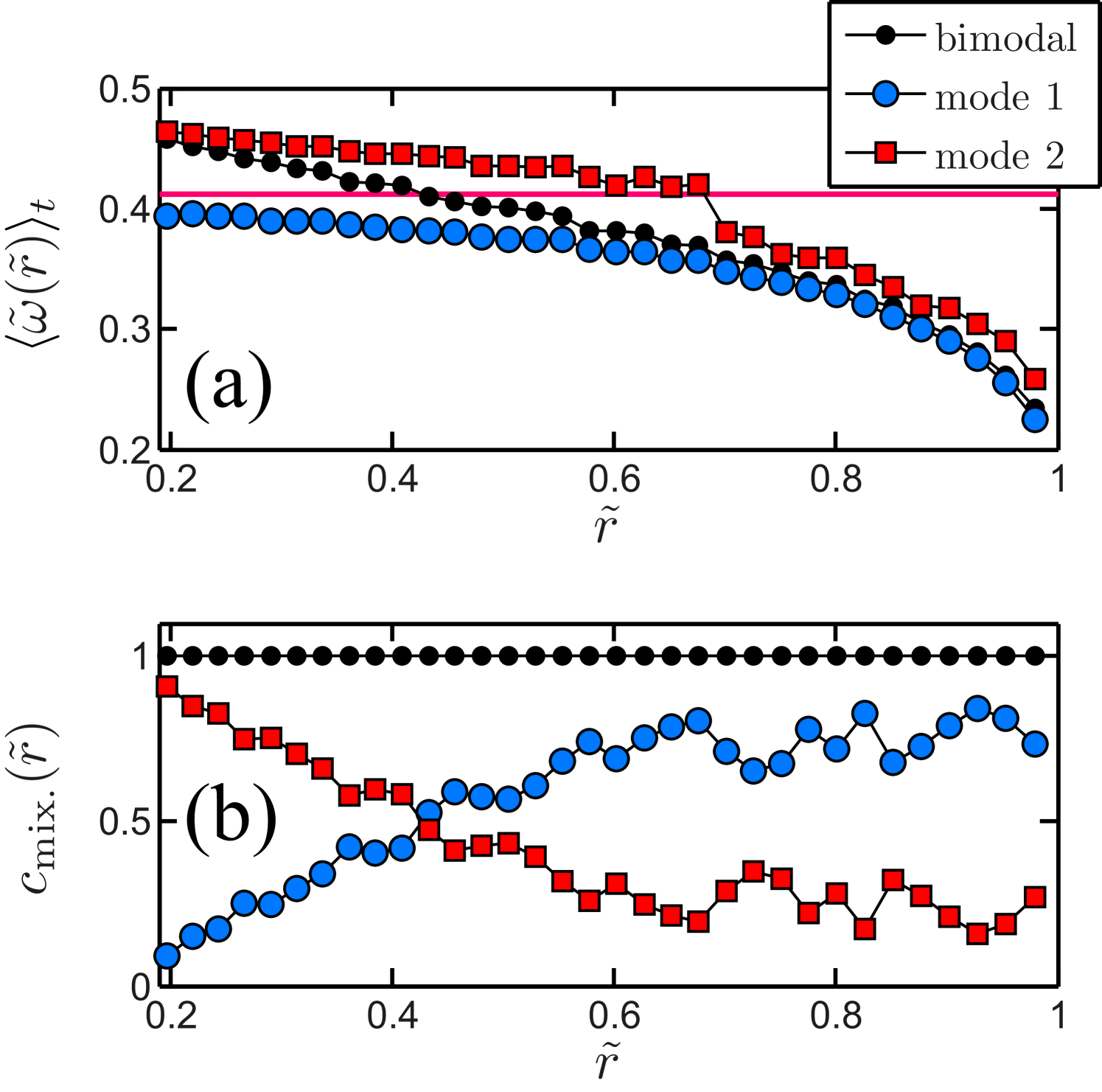
Further details on the two observed individual modes, such as their mean and their mixing coefficient, are given in figure 22 (for ) and figure 22 (for ), both well beyond . In both cases one observes that the contribution from the large- mode (dashed-dotted red curve, , apart from positions close to the outer cylinder) is, as expected, highest at the inner cylinder and fades away when going outwards, whereas the small- mode (dotted blue curve) has the reverse trend. Note, however, that, even at , e.g. relatively close to the inner cylinder, there are moments for which is negative, i.e. patches of stabilized liquids are advected inwards, just as patches of turbulent flow are advected outwards.
This mechanism resembles the angular velocity exchange mechanism suggested by Coughlin & Marcus (1996) just beyond the onset of turbulence. These authors suggest that for the counter-rotating case there is an outer region that is centrifugally stable, but subcritically unstable, thus vulnerable to distortions coming from the centrifugally unstable inner region. The inner and outer regions are separated by the neutral line. For the low of Coughlin & Marcus (1996) the inner region is not yet turbulent, but displays interpenetrating spirals, i.e. a chaotic flow with various spiral Taylor vortices. For our much larger Reynolds numbers, the inner flow will be turbulent and the distortions propagating into the subcritically unstable outer regime will be turbulent bursts. These then will lead to intermittent instabilities in the outer regime. In future work, these speculations must further be quantified.
6 Summary, discussion, and outlook
In conclusion, we have experimentally explored strongly turbulent TC flow with in the co- and counter-rotating regimes. We find that, in this large-Taylor-number regime and well off the instability lines, the dimensionless angular velocity transport flux within experimental precision can be written as with (within our accuracy) a universal for all . This is the effective scaling exponent of the ultimate regime of TC turbulence predicted by Grossmann & Lohse (2011) for RB flow and transferred to TC by the close correspondence between RB and TC elaborated in the EGL theory. When starting off counter-rotation, i.e. when increasing beyond zero, the angular velocity flux does not reduce but instead is first further enhanced, due to the enhanced shear, before finally, beyond , the stabilizing effect of the counter-rotation leads to a reduction of the angular velocity transport flux . Around the mean angular velocity profile was shown to have zero gradient in the bulk for the present large . Despite already significant counter-rotation for , there is no neutral line outside the outer BL; furthermore, the probability distribution function of the angular velocity has only one mode. For larger , beyond , a neutral line can be detected in the bulk and the p.d.f. here becomes bimodal, reflecting intermittent bursts of turbulent patches from the turbulent inner regime towards the stabilized outer regime. We offered a hypothesis that gives a unifying view and consistent understanding of all these various findings.
Clearly, the present study is only the start of a long experimental program to further explore turbulent TC flow. Much more work still must be done. In particular, we mention the following open issues:
-
•
For strong counter-rotation, i.e. large , the axial dependence must be studied in much more detail. This holds in particular for the location of the neutral line. We expect that, for large , the flow will be stabilized so much that an axial dependence of the location of the neutral line shows up again, in spite of the large numbers. It is then more appropriate to speak of a neutral surface.
-
•
Modern PIV techniques should enable us to directly resolve the inner and outer BLs.
-
•
With the help of PIV studies we also hope to visualize BL instabilities and thus better understand the dynamics of the flow, in particular, in the strongly counter-rotating case. The key question is: How does the flow manage to transport angular velocity from the turbulent inner regime towards the outer cylinder – thereby crossing the stabilized outer regime?
-
•
The studies must be repeated at lower to better understand the transition from weakly turbulent TC towards the ultimate regime as apparently seen in the present work. In our present set-up we can achieve such a regime with silicone oil instead of water.
-
•
One must also better understand the dependence of the transition to the ultimate regime.
-
•
All these studies should be complemented with direct numerical simulation of co- and counter-rotating TC flow. Just as has happened in recent years in turbulent RB flow (cf. Stevens et al. (2010, 2011)), also for turbulent TC flow we expect to narrow the gap between numerical simulation and experiment, or even to close it for not too turbulent cases, allowing for one-to-one comparisons.
-
•
Obviously, our studies must be extended to different values, in order to check the hypothesis (11) and to see how this parameter affects the flow organization.
Clearly, many exciting discoveries and wonderful work with turbulent TC flow is ahead of us.
Acknowledgements.
This study was financially supported by the Technology Foundation STW of the Netherlands, which is financially supported by NWO. The authors would like to thank G. Ahlers, H. Brauckmann, F.H. Busse, B. Eckhardt, D.P. Lathrop, R. Ostilla Mónico, M.S. Paoletti and G. Pfister for scientific discussions. D. Lohse and S. Grossmann also thank F.H. Busse for pointing them to Busse (1972) of which they were not aware when writing Eckhardt et al. (2007). We also gratefully acknowledge technical contributions from TCO-TNW Twente, G.-W. Bruggert, M. Bos, and B. Benschop.References
- Ahlers et al. (2011) Ahlers, G., Funfschilling, D. & Bodenschatz, E. 2011 Addendum to transitions in heat transport by turbulent convection at Rayleigh numbers up to . New J. Phys. 13, 049401.
- Ahlers et al. (2009) Ahlers, G., Grossmann, S. & Lohse, D. 2009 Heat transfer and large scale dynamics in turbulent Rayleigh-Bénard convection. Rev. Mod. Phys. 81, 503.
- Andereck et al. (1986) Andereck, C. D., Liu, S. S. & Swinney, H. L. 1986 Flow regimes in a circular couette system with independently rotating cylinders. J. Fluid Mech. 164, 155.
- van den Berg et al. (2003) van den Berg, T. H., Doering, C., Lohse, D. & Lathrop, D. 2003 Smooth and rough boundaries in turbulent Taylor-Couette flow. Phys. Rev. E 68, 036307.
- Borrero-Echeverry et al. (2010) Borrero-Echeverry, D., Schatz, M. F. & Tagg, R. 2010 Transient turbulence in Taylor-Couette flow. Phys. Rev. E 81, 025301.
- Bradshaw (1969) Bradshaw, P. 1969 The analogy between streamline curvature and buoyancy in turbulent shear flow. J. Fluid Mech. 36, 177–191.
- Burin et al. (2010) Burin, M. J., Schartman, E. & Ji, H. 2010 Local measurements of turbulent angular momentum transport in circular couette flow. Exp. Fluids 48, 763–769.
- Buchel et al. (1996) Buchel, P., Lucke, M., Roth, D. & Schmitz, R. 1996 Pattern selection in the absolutely unstable regime as a nonlinear eigenvalue problem: Taylor vortices in axial flow. Phys. Rev. E 53 (5), 4764–4777.
- Busse (1972) Busse, F. H. 1972 The bounding theory of turbulence and its physical significance in the case of turbulent couette flow. Statistical models and turbulence, the Springer Lecture Notes in Physics 12, 103.
- Calzavarini et al. (2005) Calzavarini, E., Lohse, D., Toschi, F. & Tripiccione, R. 2005 Rayleigh and Prandtl number scaling in the bulk of Rayleigh-Bénard turbulence. Phys. Fluids 17, 055107.
- Coles (1965) Coles, D. 1965 Transition in circular couette flow. J. Fluid Mech. 21, 385.
- Coles & van Atta (1966) Coles, D. & van Atta, C. 1966 Measured distortion of a laminar circular Couette flow by end effects. J. Fluid Mech. 25, 513.
- Coughlin & Marcus (1996) Coughlin, K. & Marcus, P. S. 1996 Turbulent Bursts in Couette-Taylor Flow. Phys. Rev. Lett. 77 (11), 2214–2217.
- DiPrima & Swinney (1981) DiPrima, R. C. & Swinney, H. L. 1981 Instabilities and transition in flow between concentric rotating cylinders. Hydrodynamic Instabilities and the Transition to Turbulence (ed. H. L. Swinney & J. P. Gollub), Springer. p. 139–180.
- Doering & Constantin (1994) Doering, C. & Constantin, P. 1994 Variational bounds on energy-dissipation in incompressible flow: shear flow. Phys. Rev. E 49, 4087–4099.
- Dominguez-Lerma et al. (1984) Dominguez-Lerma, M. A., Ahlers, G., & Cannell, D. S. 1984 Marginal stability curve and linear growth rate for rotating Couette-Taylor flow and Rayleigh-Bénard convection. Phys. Fluids 27, 856.
- Dominguez-Lerma et al. (1986) Dominguez-Lerma, M. A., Cannell, D. S. & Ahlers, G. 1986 Eckhaus boundary and wavenumber selection in rotating Couette-Taylor flow. Phys. Rev. A 34, 4956.
- Dubrulle et al. (2005) Dubrulle, B., Dauchot, O., Daviaud, F., Longgaretti, P. Y., Richard, D. & Zahn, J. P. 2005 Stability and turbulent transport in Taylor Couette flow from analysis of experimental data. Phys. Fluids 17, 095103.
- Dubrulle & Hersant (2002) Dubrulle, B. & Hersant, F. 2002 Momentum transport and torque scaling in Taylor-Couette flow from an analogy with turbulent convection. Eur. Phys. J. B 26, 379–386.
- Dutcher & Muller (2007) Dutcher, C. S. & Muller, S. J. 2007 Explicit analytic formulas for Newtonian Taylor Couette primary instabilities. Phys. Rev. E 75, 04730.
- Eckhardt et al. (2007) Eckhardt, B., Grossmann, S. & Lohse, D. 2007 Torque scaling in turbulent taylor-couette flow between independently rotating cylinders. J. Fluid Mech. 581, 221–250.
- Effinger & Grossmann (1987) Effinger, H. & Grossmann, S. 1987 Static structure function of turbulent flow from the Navier-Stokes equation. Z. Phys. B 66, 289.
- Esser & Grossmann (1996) Esser, A. & Grossmann, S. 1996 Analytic expression for Taylor-Couette stability boundary. Phys. Fluids 8, 1814–1819.
- van Gils et al. (2011a) van Gils, D. P. M., Bruggert, G. W., Lathrop, D. P., Sun, C. & Lohse, D. 2011a The Twente turbulent Taylor-Couette () facility: strongly turbulent (multi-phase) flow between independently rotating cylinders. Rev. Sci. Instr. 82, 025105.
- van Gils et al. (2011b) van Gils, D. P. M., Huisman, S. G., Bruggert, G. W., Sun, C. & Lohse, D. 2011b Torque scaling in turbulent Taylor-Couette flow with co- and counter-rotating cylinders. Phys. Rev. Lett. 106, 024502.
- Greenspan (1990) Greenspan, H. P. 1990 The theory of rotating flows. Brookline: Breukelen Press.
- Grossmann (2000) Grossmann, S. 2000 The onset of shear flow turbulence. Rev. Mod. Phys. 72, 603–618.
- Grossmann & Lohse (2000) Grossmann, S. & Lohse, D. 2000 Scaling in thermal convection: A unifying view. J. Fluid. Mech. 407, 27–56.
- Grossmann & Lohse (2001) Grossmann, S. & Lohse, D. 2001 Thermal convection for large Prandtl number. Phys. Rev. Lett. 86, 3316–3319.
- Grossmann & Lohse (2002) Grossmann, S. & Lohse, D. 2002 Prandtl and Rayleigh number dependence of the Reynolds number in turbulent thermal convection. Phys. Rev. E 66, 016305.
- Grossmann & Lohse (2004) Grossmann, S. & Lohse, D. 2004 Fluctuations in turbulent Rayleigh-Bénard convection: The role of plumes. Phys. Fluids 16, 4462–4472.
- Grossmann & Lohse (2011) Grossmann, S. & Lohse, D. 2011 Multiple scaling in the ultimate regime of thermal convection. Phys. Fluids 23, 045108.
- He et al. (2012) He, X., Funfschilling, D., Nobach, H., Bodenschatz, E. & Ahlers, G. 2012 Transition to the ultimate state of turbulent Rayleigh-Bénard convection. Phys. Rev. Lett. 108, 024502.
- Hollerbach & Fournier (2004) Hollerbach, R. & Fournier, A. 2004 End-effects in rapidly rotating cylindrical Taylor-Couette flow. In MHD Couette flows: experiments and models (ed. Rosner, R and Rudiger, G and Bonanno, A), AIP Conference Proceedings, vol. 733, pp. 114–121. INAF; Catania Univ; Banca Roma, American Inst. Phys., Workshop on MHD Couette Flows, Acitrezza, Italy, Feb. 29-MAR 02, 2004.
- van Hout & Katz (2011) van Hout, R. & Katz, J. 2011 Measurements of mean flow and turbulence characteristics in high-Reynolds number counter-rotating Taylor-Couette flow. Phys. Fluids 23 (10), 105102.
- Huisman et al. (2012a) Huisman, S. G., van Gils, D. P. M., Grossmann, S., Sun, C. & Lohse, D. 2012a Ultimate turbulent Taylor-Couette flow. Phys. Rev. Lett. 108, 024501.
- Huisman et al. (2012b) Huisman, S. G., van Gils, D. P. M. & Sun, C. 2012b Applying laser doppler anemometry inside a Taylor-Couette geometry using a ray-tracer to correct for curvature effects. European J. Mech. B/Fluids In press.
- Ji et al. (2006) Ji, H., Burin, M., Schartman, E. & Goodman, J. 2006 Hydrodynamic turbulence cannot transport angular momentum effectively in astrophysical disks. Nature 444, 343–346.
- Kraichnan (1962) Kraichnan, R. H. 1962 Turbulent thermal convection at arbritrary Prandtl number. Phys. Fluids 5, 1374–1389.
- Landau & Lifshitz (1987) Landau, L. D. & Lifshitz, E. M. 1987 Fluid Mechanics. Oxford: Pergamon Press.
- Lathrop et al. (1992a) Lathrop, D. P., Fineberg, J. & Swinney, H. S. 1992a Transition to shear-driven turbulence in Couette-Taylor flow. Phys. Rev. A 46, 6390–6405.
- Lathrop et al. (1992b) Lathrop, D. P., Fineberg, J. & Swinney, H. S. 1992b Turbulent flow between concentric rotating cylinders at large Reynolds numbers. Phys. Rev. Lett. 68, 1515–1518.
- Lewis & Swinney (1999) Lewis, G. S. & Swinney, H. L. 1999 Velocity structure functions, scaling, and transitions in high-Reynolds-number Couette-Taylor flow. Phys. Rev. E 59, 5457–5467.
- Lohse & Toschi (2003) Lohse, D. & Toschi, F. 2003 The ultimate state of thermal convection. Phys. Rev. Lett. 90, 034502.
- Marcus (1984) Marcus, P. S. 1984 Simulation of taylor-couette flow. part 1. numerical methods and comparison with experiment. J. Fluid Mech. 146, 45 – 64.
- Mullin et al. (1987) Mullin, T., Cliffe, K. A. & Pfister, G. 1987 Unusual time-dependent phenomena in Taylor-Couette flow at moderately low Reynolds numbers. Phys. Rev. Lett. 58 (21), 2212–2215.
- Mullin et al. (1982) Mullin, T., Pfister, G. & Lorenzen, A. 1982 New observations on hysteresis effects in Taylor-Couette flow. Phys. Fluids 25 (7), 1134–1136.
- Ostilla et al. (2012) Ostilla, R., Stevens, R. J. A. M., Grossmann, S., Verzicco, R. & Lohse, D. 2012 Optimal Taylor-Couette flow: transition to turbulence. J. Fluid Mech., prepint.
- Paoletti & Lathrop (2011) Paoletti, M. S. & Lathrop, D. P. 2011 Angular momentum transport in turbulent flow between independently rotating cylinders. Phys. Rev. Lett. 106, 024501.
- Pfister & Rehberg (1981) Pfister, G. & Rehberg, I. 1981 Space dependent order parameter in circular Couette flow transitions. Phys. Lett. 83, 19–22.
- Pfister et al. (1988) Pfister, G., Schmidt, H., Cliffe, K. A. & Mullin, T. 1988 Bifurcation phenomena in taylor-couette flow in a very short annulus. J. Fluid Mech. 191, 1–18.
- Ravelet et al. (2010) Ravelet, F., Delfos, R. & Westerweel, J. 2010 Influence of global rotation and reynolds number on the large-scale features of a turbulent taylor–couette flow. Phys. Fluids 22 (5), 055103.
- Richard (2001) Richard, D. 2001 Instabilités Hydrodynamiques dans les Ecoulements en Rotation Différentielle. PhD thesis, Université Paris VII.
- Roche et al. (2001) Roche, P. E., Castaing, B., Chabaud, B. & Hebral, B. 2001 Observation of the 1/2 power law in Rayleigh-Bénard convection. Phys. Rev. E 63, 045303.
- Schmidt et al. (2012) Schmidt, L. E., Calzavarini, E., Lohse, D., Toschi, F. & Verzicco, R. 2012 Axially homogeneous Rayleigh-Bénard convection in a cylindrical cell. J. Fluid Mech. 691, 52–68.
- Smith & Townsend (1982) Smith, G. P. & Townsend, A. A. 1982 Turbulent Couette flow between concentric cylinders at large Taylor numbers. J. Fluid Mech. 123, 187–217.
- Stevens et al. (2011) Stevens, R. J. A. M., Lohse, D. & Verzicco, R. 2011 Prandtl and Rayleigh number dependence of heat transport in high Rayleigh number thermal convection. J. Fluid Mech. 688, 31–43.
- Stevens et al. (2010) Stevens, R. J. A. M., Verzicco, R. & Lohse, D. 2010 Radial boundary layer structure and Nusselt number in Rayleigh-Bénard convection. J. Fluid Mech. 643, 495–507.
- Sugiyama et al. (2007) Sugiyama, K., Calzavarini, E., Grossmann, S. & Lohse, D. 2007 Non-Oberbeck-Boussinesq effects in Rayleigh-Bénard convection:beyond boundary-layer theory. Europhys. Lett. 80, 34002.
- Sun et al. (2008) Sun, C., Cheung, Y. H. & Xia, K.-Q. 2008 Experimental studies of the viscous boundary layer properties in turbulent Rayleigh-Bénard convection. J. Fluid Mech. 605, 79 – 113.
- Tagg (1994) Tagg, R. 1994 The Couette-Taylor problem. Nonlinear Science Today 4 (3), 1.
- Taylor (1923) Taylor, G. I. 1923 Stability of a viscous liquid contained between two rotating cylinders. Philos. Trans. R. Soc. London A 223, 289.
- Wendt (1933) Wendt, F. 1933 Turbulente Strömungen zwischen zwei rotierenden Zylindern. Ingenieurs-Archiv 4, 577–595.
- Werne (1994) Werne, J. 1994 Plume model for boundary layer dynamics in hard turbulence. Phys. Rev. E 49, 4072.
- Zhou et al. (2010) Zhou, Q., Stevens, R. J. A. M., Sugiyama, K., Grossmann, S., Lohse, D. & Xia, K.-Q. 2010 Prandtl-Blasius temperature and velocity boundary layer profiles in turbulent Rayleigh-Bénard convection. J. Fluid Mech. 664, 297.