\optauthor\Name

Jung Hun Oh \Emailohj@mskcc.org
\addrDepartment of Medical Physics, Memorial Sloan Kettering Cancer Center, New York, NY, USA and \NameRena Elkin \Emailelkinr@mskcc.org
\addrDepartment of Medical Physics, Memorial Sloan Kettering Cancer Center, New York, NY, USA and \NameAnish K. Simhal \Emailsimhala@mskcc.org
\addrDepartment of Medical Physics, Memorial Sloan Kettering Cancer Center, New York, NY, USA and \NameJiening Zhu \Emailjiening.zhu@stonybrook.edu
\addrDepartment of Applied Mathematics & Statistics, Stony Brook University, Stony Brook, NY, USA and \NameJoseph O. Deasy \Emaildeasyj@mskcc.org
\addrDepartment of Medical Physics, Memorial Sloan Kettering Cancer Center, New York, NY, USA and \NameAllen Tannenbaum \Emailallen.tannenbaum@stonybrook.edu
\addrDepartments of Computer Science and Applied Mathematics & Statistics, Stony Brook University, Stony Brook, NY, USA

Optimal Transport for Kernel Gaussian Mixture Models

Abstract

The Wasserstein distance from optimal mass transport (OMT) is a powerful mathematical tool with numerous applications that provides a natural measure of the distance between two probability distributions. Several methods to incorporate OMT into widely used probabilistic models, such as Gaussian or Gaussian mixture, have been developed to enhance the capability of modeling complex multimodal densities of real datasets. However, very few studies have explored the OMT problems in a reproducing kernel Hilbert space (RKHS), wherein the kernel trick is utilized to avoid the need to explicitly map input data into a high-dimensional feature space. In the current study, we propose a Wasserstein-type metric to compute the distance between two Gaussian mixtures in a RKHS via the kernel trick, i.e., kernel Gaussian mixture models.

1 Introduction

The Gaussian mixture model (GMM) is a probabilistic model defined as a weighted sum of several Gaussian distributions (Moraru et al., 2019; Dasgupta and Schulman, 2000). Due to its mathematical simplicity and efficiency, GMMs are widely used to model complex multimodal densities of real datasets (Delon and Desolneux, 2020).

Optimal mass transport (OMT) is an active and ever-growing field of research, originating in the work of the French civil engineer Gaspard Monge in 1781, which was formulated as the optimal way (via the minimization of some transportation cost) to move a pile of soil from one site to another (Evans, 1999; Villani, 2003; Kantorovich, 2006; Pouryahya et al., 2022). OMT has made significant progress due to the pioneering effort of Leonid Kantorovich in 1942, who introduced a relaxed version of the original problem that is solved using simple linear programming (Kantorovich, 2006). Recently, there has been an ever increasing growth in applications of OMT in numerous fields, including medical imaging analysis, statistical physics, machine learning, and genomics (Chen et al., 2017, 2019; Luise et al., 2018; Zhao et al., 2013).

Here we briefly sketch the basic theory of OMT. Suppose that $\nu_{0}$ and $\nu_{1}$ are two absolutely continuous probability measures with compact support on $X=\mathbb{R}^{d}$ . (The theory is valid on more general metric measure spaces.) A Borel map $T:X\rightarrow X$ is called a transport plan from $\nu_{0}$ to $\nu_{1}$ if it “push-forward” $\nu_{0}$ to $\nu_{1}$ ( $T_{\#}\nu_{0}=\nu_{1}$ ) which is equivalent to say that

\nu_{1}(B)=\nu_{0}(T^{-1}(B)),

(1)

for every Borel subset $B\subset\mathbb{R}^{d}$ (Kolouri et al., 2019; Lei et al., 2019). Let $c(x,y)$ be the transportation cost to move one unit of mass from $x$ to $y$ . The Monge version of OMT problem seeks an optimal transport map $T:X\rightarrow X$ such that the total transportation cost $\int_{X}c(x,T(x)){\nu_{0}}(dx)$ is minimized over the set of all transport maps $T$ . We note that the original OMT problem is highly non-linear and may not admit a viable solution. To ease this computational difficulty, Leonid Kantorovich proposed a relaxed formulation, solved by employing a linear programming method (Kantorovich, 2006; Shi et al., 2021) which defines the $\textit{W}_{p}$ Wasserstein distance between $\nu_{0}$ and $\nu_{1}$ on $\mathbb{R}^{d}$ as follows:

W_{p}^{p}\left({\nu_{0}},{\nu_{1}}\right)=\inf\limits_{\pi\in\Pi(\nu_{0},\nu_{1})}\int_{{\mathbb{R}}^{d}\times{\mathbb{R}}^{d}}{\|{x}-{y}\|}^{p}d\pi(x,y),

(2)

where $\Pi(\nu_{0},\nu_{1})$ is the set of all joint probability measures $\pi$ on $X\times X$ with $\nu_{0}$ and $\nu_{1}$ as its two marginals, and $c(x,y)$ is taken as a specific form of $c(x,y)=||x-y||^{p},p\geq 1$ . In the present study, we focus on the $\textit{W}_{2}$ Wasserstein distance using the squared Euclidean distance ( $p=2$ ) as the cost function (Mallasto and Feragen, 2017).

While OMT ensures that the displacement interpolation (weighted barycenters) between two Gaussian distributions remains Gaussian, this property does not hold for Gaussian mixtures. To cope with this issue in GMMs, Chen ${\it et~{}al.}$ proposed a new Wasserstein-type distance (Chen et al., 2019). This approach optimizes the transport map between the two probability vectors of the respective Gaussian mixtures using the discrete linear program where the cost function is computed as the closed-form formulation of the $W_{2}$ Wasserstein distance between Gaussian distributions. This ensures that the displacement interpolation between two Gaussian mixtures preserves the Gaussian mixture structure. Note that the sum of probabilities of all Gaussian components in a Gaussian mixture is 1, and therefore the total mass for two Gaussian mixtures is equal.

In machine learning, kernel methods provide a powerful framework for non-linear extensions of classical linear models by implicitly mapping the data into a high-dimensional feature space corresponding to a reproducing kernel Hilbert space (RKHS) via a non-linear mapping function (Meanti et al., 2020; Simon-Gabriel and Schölkopf, 2018; Oh and Gao, 2009). Recently, a formulation for the $W_{2}$ Wasserstein distance metric between two Gaussian distributions in a RKHS was introduced (Oh et al., 2019, 2020; Zhang et al., 2020). Extending this concept, we propose an OMT framework to compute a Wasserstein-type distance between two Gaussian mixtures in a RKHS.

2 Methods

In this section, we first describe the underlying technical methods of the present work, and then introduce our proposed methodology.

2.1 Kernel function

Suppose that we are given a dataset of $n$ samples, denoted by $X=[x_{1},x_{2},\cdots,x_{\it n}]\in\mathbb{R}^{d}$ , each of which consists of $d$ features. The data in the original input space can be mapped into a high-dimensional feature space via a non-linear mapping function $\phi$ (Baudat and Anouar, 2000; Oh and Gao, 2011; Kwon and Nasrabadi, 2005):

\Phi:X\rightarrow\mathcal{F},

(3)

where $\mathcal{F}$ is a Hilbert space called the feature space and a (Mercer) kernel function $k({x_{i},x_{j}})=\langle\phi{(x_{i})},\phi{(x_{j})}\rangle=\phi(x_{i})^{\rm T}\phi(x_{j})$ is defined as an inner dot product in $\mathcal{F}$ for a positive semi-definite kernel $k:X\times X\rightarrow\mathbb{R}$ in which the kernel function is symmetric: $k(x_{i},x_{j})=k(x_{j},x_{i})$ and $\Phi(X):=[\phi(x_{1}),\phi(x_{2}),\cdots,\phi(x_{n})]$ (Schölkopf, 2000; Rahimi and Recht, 2007). The resulting Gram matrix $K=\Phi^{\rm T}\Phi$ is positive semi-definite ( $K\succeq 0$ ) with $K_{ij}:=k(x_{i},x_{j}),\forall i,j\in\{1,\cdots,n\}$ . This process is called the kernel trick. Common choices of kernel functions are the Gaussian radial basis function (RBF) and polynomial kernels (Kolouri et al., 2016; Shi et al., 2018; Pilario et al., 2020). Kernels are widely used in machine learning algorithms such as support vector machines (Chen et al., 2007), linear discriminant analysis (Oh and Gao, 2011), and principal component analysis (Schölkopf et al., 1999; Sterge et al., 2020). In this study, the following RBF kernel is employed:

k({x_{i},x_{j}})=\mathrm{exp}\big{(}-\gamma||{x_{i}-x_{j}}||^{2}\big{)},

(4)

where $\gamma>0$ controls the kernel width. The mean and the covariance matrix in the feature space are given by

\it m=\frac{\rm 1}{n}\sum_{i={\rm 1}}^{n}\phi(x_{\it i})={\rm{\Phi}{\it s}},~{}~{}{\rm\Sigma}=\frac{\rm 1}{n}\sum_{i={\rm 1}}^{n}(\phi(x_{\it i})-{\it m})(\phi(x_{\it i})-{\it m})^{\rm T}={\rm{\Phi}{\it JJ}^{\rm T}\rm{\Phi}^{\rm T}},

(5)

where $s_{n\times 1}=\frac{1}{n}{\vec{1}}^{\rm T}$ , ${J}=\frac{\rm 1}{\sqrt{\it{n}}}(I_{\it n}-s{\vec{1}})$ , ${\vec{1}}=[1,1,\cdots,1]$ , and $I_{n}$ is the $n\times n$ identity matrix. Then, denoting ${\Phi J}$ by $S$ , we have

{S=\Phi J}=\frac{\rm 1}{\sqrt{\it n}}[(\phi({x}_{\rm 1})-\it m),\cdots,(\phi({x}_{\it n})-\it m)].

(6)

A key idea to compute a Wasserstein-type distance between two Gaussian mixtures in a RKHS is to efficiently convert the mapping functions represented by $\it m$ and $\Sigma$ to kernel functions by putting two mapping functions next to each other in a certain way.

2.2 OMT between Gaussian distributions

Given two Gaussian distributions, $\nu_{0}$ and $\nu_{1}\in\mathbb{R}^{\it d}$ , with mean $\theta_{i}$ and covariance matrix $\it C_{i}$ for $i=0$ and 1, the $W_{2}$ Wasserstein distance between the two distributions has the following closed formula:

W_{2}(\nu_{0},\nu_{1})^{2}=\|{\theta}_{\rm 0}-{\theta}_{\rm 1}\|^{2}+\\ \mathrm{tr}\left({\it C}_{0}+{\it C}_{1}-2\left({\it C}_{0}^{\frac{1}{2}}{\it C}_{1}{\it C}_{0}^{\frac{1}{2}}\right)^{\frac{1}{2}}\right),

(7)

where tr is the trace and $\mathrm{tr}\left({\it C}_{0}+{\it C}_{1}-2({\it C}_{0}^{\frac{1}{2}}{\it C}_{1}{\it C}_{0}^{\frac{1}{2}})^{\frac{1}{2}}\right)=\mathrm{tr}\left({\it C}_{0}+{\it C}_{1}-2({\it C}_{1}{\it C}_{0})^{\frac{1}{2}}\right)$ . In particular, when ${\it C}_{0}={\it C}_{1}$ , we have $W_{2}(\nu_{0},\nu_{1})^{2}=\|{\theta}_{\rm 0}-{\theta}_{\rm 1}\|^{2}.$ If ${\it C_{0}}$ and ${\it C_{1}}$ are non-degenerate, the geodesic path (displacement interpolation) $(\nu_{t})_{t\in[0,1]}$ between $\nu_{0}$ and $\nu_{1}$ remains Gaussian and satisfies

\nu_{t}\in{\rm argmin}_{\rho}(1-t)W_{2}(\nu_{0},\rho)^{2}+tW_{2}(\nu_{1},\rho)^{2},

(8)

with mean $\theta_{t}=(1-t)\theta_{\rm 0}+t{\theta}_{\rm 1}$ and covariance matrix given by:

C_{t}=((1-t)I_{d}+tQ)C_{0}((1-t)I_{d}+tQ),

(9)

where $I_{d}$ is the $d\times d$ identity matrix and $Q=C_{1}^{\frac{1}{2}}(C_{1}^{\frac{1}{2}}C_{0}C_{1}^{\frac{1}{2}})^{-{\frac{1}{2}}}C_{1}^{\frac{1}{2}}$ (Delon and Desolneux, 2020).

2.3 OMT between Gaussian distributions in a RKHS

The data distribution in a RKHS represented via proper kernel functions is assumed to approximately follow a Gaussian distribution under suitable conditions, as justified by Huang ${\it et~{}al.}$ (Huang et al., 2005). Let $\rho_{0}$ and $\rho_{1}\in\mathbb{R}^{\it l}$ be two Gaussian distributions in a RKHS with mean ${\it m}_{\it i}$ and covariance matrix ${\Sigma}_{\it i}$ for $i=0,1$ . The $W_{2}$ Wasserstein distance in a RKHS, denoted as $KW_{2}$ (kernel Wasserstein distance), is then defined as follows:

KW_{2}(\rho_{0},\rho_{1})^{2}=\|{\it m}_{\rm 0}-{\it m}_{\rm 1}\|^{2}+\\ \mathrm{tr}\left({\Sigma}_{0}+\Sigma_{1}-2\left({\Sigma}_{0}^{\frac{1}{2}}{\Sigma}_{1}{\Sigma}_{0}^{\frac{1}{2}}\right)^{\frac{1}{2}}\right),

(10)

where $\Sigma_{i}^{\frac{1}{2}}$ is the unique semi-definite positive square root of a symmetric semi-definite positive matrix $\Sigma_{i}$ (Xia et al., 2014; Delon et al., 2022).

Suppose that there are two sets of data in the original input space, ${X}=[{x}_{1},{x}_{2},\cdots,{x}_{\it n}]$ and ${Y}=[{y}_{1},{y}_{2},\cdots,{y}_{\it m}]\in\mathbb{R}^{d}~{}(d<l)$ , associated with $\rho_{0}$ and $\rho_{1}$ , respectively. The first term in Eq. (10) is the squared maximum mean discrepancy (MMD) (Iyer et al., 2014; Ouyang and Key, 2021) and may be expressed with kernel functions as follows:

\|{\it m}_{0}-{\it m}_{1}\|^{2}=\frac{1}{n^{2}}\sum_{i=1}^{n}\sum_{j=1}^{n}{\it k}\left({x}_{i},{x}_{j}\right)-\frac{2}{nm}\sum_{i=1}^{n}\sum_{j=1}^{m}{\it k}\left({x}_{i},{y}_{j}\right)+\frac{1}{m^{2}}\sum_{i=1}^{m}\sum_{j=1}^{m}{\it k}\left({y}_{i},{y}_{j}\right).

(11)

By using Eq. (5), the second term in Eq. (10) is expressed as follows:

	$\displaystyle\mathrm{tr}\left({\Sigma}_{0}+\Sigma_{1}-2\left({\Sigma}_{0}^{\frac{1}{2}}{\Sigma}_{1}{\Sigma}_{0}^{\frac{1}{2}}\right)^{\frac{1}{2}}\right)=\mathrm{tr}\left({\Sigma}_{0}+\Sigma_{1}-2\left({\Sigma}_{1}{\Sigma}_{0}\right)^{\frac{1}{2}}\right)~{}~{}~{}~{}~{}~{}~{}~{}~{}~{}$		(12)
	$\displaystyle=\mathrm{tr}\left(J_{0}J_{0}^{\rm T}{\Phi}_{0}^{\rm T}{\Phi}_{0}\right)+\mathrm{tr}\left(J_{1}J_{1}^{\rm T}{\Phi}_{1}^{\rm T}{\Phi}_{1}\right)-2\mathrm{tr}\left({\Phi}_{1}J_{1}J_{1}^{\rm T}K_{10}J_{0}J_{0}^{\rm T}{\Phi}_{0}^{\rm T}\right)^{\frac{1}{2}}$
	$\displaystyle=\mathrm{tr}\left({J}_{0}{J}_{0}^{\rm T}{K}_{00}\right)+\mathrm{tr}\left({J}_{1}{J}_{1}^{\rm T}{{K}_{11}}\right)-2\mathrm{tr}\left({\Phi}_{1}{Q}{\Phi}_{0}^{\rm T}\right)^{\frac{1}{2}},~{}~{}~{}~{}~{}~{}~{}~{}~{}~{}~{}~{}~{}~{}~{}~{}~{}~{}~{}~{}~{}~{}~{}~{}~{}~{}$

where $\mathrm{tr}\left({\Phi}_{1}{Q}{\Phi}_{0}^{\rm T}\right)^{\frac{1}{2}}=\mathrm{tr}\left({K}_{01}{J}_{1}{J}_{1}^{\rm T}{K}_{10}{J}_{0}{J}_{0}^{\rm T}\right)^{\frac{1}{2}}$ , ${Q}={J}_{1}{J}_{1}^{\rm T}{K}_{10}{J}_{0}{J}_{0}^{\rm T}$ , and ${K}_{\it ij}={\Phi}_{i}^{\rm T}{\Phi_{\it j}}$ . Note that ${\Sigma_{\rm 0}}$ and ${\Sigma_{\rm 1}}$ are symmetric positive semi-definite. Plugging the two terms together into Eq. (10), the ${\it KW_{\rm 2}}$ distance between $\rho_{0}$ and $\rho_{1}$ may be expressed as:

	$\displaystyle KW_{2}(\rho_{0},\rho_{1})^{2}=\frac{1}{n^{2}}\sum_{i=1}^{n}\sum_{j=1}^{n}{\it k}\left({x}_{i},{x}_{j}\right)-\frac{2}{nm}\sum_{i=1}^{n}\sum_{j=1}^{m}{\it k}\left({x}_{i},{y}_{j}\right)+\frac{1}{m^{2}}\sum_{i=1}^{m}\sum_{j=1}^{m}{\it k}\left({y}_{i},{y}_{j}\right)+$		(13)
	$\displaystyle\mathrm{tr}\left({J}_{0}{J}_{0}^{\rm T}{K}_{00}\right)+\mathrm{tr}\left({J}_{1}{J}_{1}^{\rm T}{K}_{11}\right)-2\mathrm{tr}\left({K}_{01}{J}_{1}{J}_{1}^{\rm T}{K}_{10}{J}_{0}{J}_{0}^{\rm T}\right)^{\frac{1}{2}}.$

Eq. (13) will be used as a key component for the computation of a Wasserstein-type distance between two Gaussian mixtures in a RKHS in the following section. In the special case, when ${\Sigma}_{0}={\Sigma}_{1}$ , we have $KW_{2}(\rho_{0},\rho_{1})^{2}=\frac{1}{n^{2}}\sum_{i=1}^{n}\sum_{j=1}^{n}{\it k}\left({x}_{i},{x}_{j}\right)-\frac{2}{nm}\sum_{i=1}^{n}\sum_{j=1}^{m}{\it k}\left({x}_{i},{y}_{j}\right)+\\ \frac{1}{m^{2}}\sum_{i=1}^{m}\sum_{j=1}^{m}{\it k}\left({y}_{i},{y}_{j}\right)$ .

2.4 OMT between GMMs in a RKHS

Based on the OMT method between GMMs introduced in (Chen et al., 2019), we propose a Wasserstein-type metric to compute the distance between two Gaussian mixtures in a RKHS via the kernel trick, which preserves the Gaussian mixture structure in the displacement interpolation. Let $\mu$ be a Gaussian mixture in a RKHS:

\displaystyle\mu=\sum_{k=1}^{N}p^{k}v^{k},

(14)

where each $v^{k}$ is a Gaussian distribution in a RKHS with $v^{k}=\mathcal{N}(m_{k},\Sigma_{k})$ and $p^{k}$ is a probability of $v^{k}$ with $\sum_{k=1}^{N}p^{k}=1$ . Let $\mu_{0}$ and $\mu_{1}$ denote two Gaussian mixtures in a RKHS in the following form:

\displaystyle\mu_{i}=p_{i}^{1}v_{i}^{1}+p_{i}^{2}v_{i}^{2}+...+p_{i}^{N_{i}}v_{i}^{N_{i}},\quad i=0,1,

(15)

where $N_{i}$ is the number of Gaussian components of $\mu_{i}$ . The distance between $\mu_{0}$ and $\mu_{1}$ is then defined according to the discrete OMT formulation for discrete measures (Chen et al., 2019; Mathews et al., 2020):

\displaystyle d(\mu_{0},\mu_{1})^{2}=\min\limits_{\pi\in\Pi(p_{0},p_{1})}\sum_{i,j}c_{ij}\pi_{ij},

(16)

where $\Pi(p_{0},p_{1})$ is the set of all joint probability measures between $p_{0}$ and $p_{1}$ , defined as:

\displaystyle\Pi(p_{0},p_{1})=\{\pi\in\mathbb{R}_{+}^{N_{0}\times N_{1}}|\sum_{j}\pi_{kj}=p_{0}^{k},~{}\sum_{k}\pi_{kj}=p_{1}^{j}\}.

The cost $c_{ij}$ is taken to be the square of the $KW_{2}$ distance between $v_{0}^{i}$ and $v_{1}^{j}$ in a RKHS:

\displaystyle c_{ij}=KW_{2}(v_{0}^{i},v_{1}^{j})^{2}.

(17)

Since $v_{0}^{i}$ and $v_{1}^{j}$ are Gaussian distributions in a RKHS, the $KW_{2}$ distance can be computed using Eq. (13). Let $\pi^{*}$ be the optimal solution of Eq. (16). Then, the distance $d(\mu_{0},\mu_{1})$ between two Gaussian mixtures in a RKHS is defined as follows:

\displaystyle d(\mu_{0},\mu_{1})=\sqrt{\sum_{i,j}c_{ij}\pi_{ij}^{*}},

(18)

where $d(\mu_{0},\mu_{1})\geq KW_{2}(\mu_{0},\mu_{1})$ and the following property holds (Chen et al., 2019):

\displaystyle d(\mu_{s},\mu_{t})=(t-s)d(\mu_{0},\mu_{1}),\quad 0\leq s<t\leq 1.

(19)

The geodesic path $\mu_{t}$ between $\mu_{0}$ and $\mu_{1}$ is defined as

\displaystyle\mu_{t}=\sum_{i,j}\pi_{ij}^{*}v_{t}^{ij},

(20)

where $v_{t}^{ij}$ is the displacement interpolation between two Gaussian distributions, $v_{0}^{i}$ and $v_{1}^{j}$ .

3 Experiments

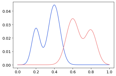
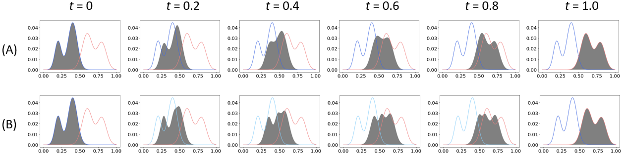
Suppose that we are given two Gaussian mixtures, $\mu_{0}=0.3\mathcal{N}(0.2,0.002)+0.7\mathcal{N}(0.4,0.004)$ and $\mu_{1}=0.6\mathcal{N}(0.6,0.005)+0.4\mathcal{N}(0.8,0.004)$ as a 1-dimensional example, as shown in Figure 11. Figure 22 shows the displacement interpolation $\mu_{t}$ for both the metric $d(\mu_{0},\mu_{1})$ and general Wasserstein distance between the $\mu_{0}$ and $\mu_{1}$ at $t$ = 0, 0.2, 0.4, 0.6, 0.8, and 1.0. It is observed that the displacement interpolation for the metric $d(\mu_{0},\mu_{1})$ preserves the Gaussian mixture structure, whereas the displacement interpolation for the general Wasserstein distance does not.

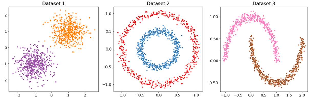
As another example, three datasets were generated in the original input space, each of which has two distributions (Figure 33). Each dataset consists of 1,000 data points with 500 data points for each distribution. The $d(\cdot,\cdot)$ was then computed between each pair of datasets in a RKHS, assuming that each dataset ( $\mu_{0},\mu_{1}$ , and $\mu_{2}$ ) has two Gaussian components with $v_{0}^{1}$ (purple)/ $v_{0}^{2}$ (orange), $v_{1}^{1}$ (red)/ $v_{1}^{2}$ (blue), and $v_{2}^{1}$ (pink)/ $v_{2}^{2}$ (brown), respectively in a RKHS (Tables 1 and 2). In the current study, $\gamma=1$ (Table 1) and $\gamma=10$ (Table 2) were used in the RBF kernel shown in Eq. (4).

The $d(\cdot,\cdot)$ values with $\gamma=10$ were larger than those corresponding to $\gamma=1$ . Overall, the $d(\cdot,\cdot)$ values between dataset 2 and dataset 3 were smaller than dataset 1 vs. dataset 2 and dataset 1 vs. dataset 3. When $\gamma=1$ and $(p_{0}^{1},p_{0}^{2})$ is (0.1, 0.9) and (0.3, 0.7), the $d(\cdot,\cdot)$ values between dataset 1 and dataset 2 were larger than those between dataset 1 and dataset 3. By contrast, when $(p_{0}^{1},p_{0}^{2})$ is one of (0.5, 0.5), (0.7, 0.3), and (0.9, 0.1), the $d(\cdot,\cdot)$ values between dataset 1 and dataset 2 were smaller than those between dataset 1 and dataset 3. When $\gamma=10$ , the $d(\cdot,\cdot)$ values between dataset 1 and dataset 3 were larger than those between dataset 1 and dataset 2 in more cases compared to when $\gamma=1$ .

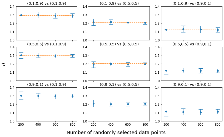
Using dataset 1 and dataset 2, simulation tests were conducted with (0.1, 0.9), (0.5, 0.5), and (0.9, 0.1) for both $(p_{0}^{1},p_{0}^{2})$ and $(p_{1}^{1},p_{1}^{2})$ by randomly sampling 200, 400, 600, and 800 data points from 1,000 data points of each dataset. For each sampling experiment of the combination of $(p_{0}^{1},p_{0}^{2})$ and $(p_{1}^{1},p_{1}^{2})$ , 100 tests were conducted and the average distance and standard deviation were computed. In Figure 44, the horizontal dot line indicates $d(\cdot,\cdot)$ when the original data with 1,000 data points for each dataset were analyzed. As can be seen, as the number of randomly selected data points increases, the standard deviation becomes narrower, converging to the horizontal dot line. Not surprisingly, the average distance after 100 repetitions of each sampling experiment was very similar to $d(\cdot,\cdot)$ computed on the original data with 1,000 data points for each dataset.

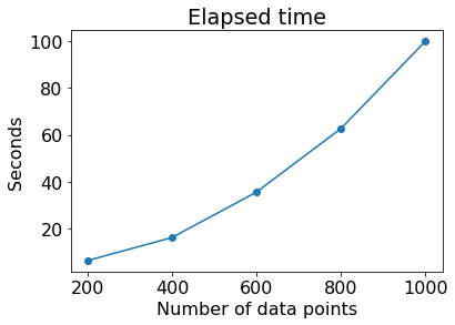
Figure 55 illustrates the elapsed time to compute $d(\cdot,\cdot)$ between dataset 1 and dataset 2 when each test was conducted only once with randomly sampled data points (200, 400, 600, 800) from each dataset, compared to the elapsed time in the original datasets (each 1,000 data points). As the number of data points increased, the computational time to compute $d(\cdot,\cdot)$ sharply increased. Therefore, there is a tradeoff between the computational time and the precision of computed distance in the sampling approach. Use of advanced sampling techniques will help compute the distance within reasonable computational time and with minimal error. All experiments in the current study were carried out using Python language in Google Colab-Pro environment.

\acks

This study was supported in part by National Institutes of Health (NIH)/National Cancer Institute Cancer Center support grant (P30 CA008748), NIH grant (R01-AG048769), AFOSR grant (FA9550-20-1-0029), Army Research Office grant (W911NF2210292), Breast Cancer Research Foundation grant (BCRF-17-193), and a grant from the Cure Alzheimer’s Foundation.

References

Baudat and Anouar (2000) Gaston Baudat and Fatiha Anouar. Generalized discriminant analysis using a kernel approach. Neural Computation, 12(10):2385–2404, 2000.
Chen et al. (2017) Yongxin Chen, Filemon Dela Cruz, Romeil Sandhu, Andrew L. Kung, Prabhjot Mundi, Joseph O. Deasy, and Allen Tannenbaum. Pediatric sarcoma data forms a unique cluster measured via the earth mover’s distance. Scientific Reports, 7(1):7035, 2017.
Chen et al. (2019) Yongxin Chen, Tryphon T. Georgiou, and Allen Tannenbaum. Optimal transport for gaussian mixture models. IEEE Access, 7:6269–6278, 2019.
Chen et al. (2007) Zhenyu Chen, Jianping Li, and Liwei Wei. A multiple kernel support vector machine scheme for feature selection and rule extraction from gene expression data of cancer tissue. Artificial Intelligence in Medicine, 41(2):161–175, 2007.
Cuturi (2013) Marco Cuturi. Sinkhorn distances: Lightspeed computation of optimal transport. Advances in Neural Information Processing Systems (NeurIPS), pages 2292–2300, 2013.
Dasgupta and Schulman (2000) Sanjoy Dasgupta and Leonard J. Schulman. A two-round variant of em for gaussian mixtures. The Conference on Uncertainty in Artificial Intelligence (UAI), pages 152–159, 2000.
Delon and Desolneux (2020) Julie Delon and Agnès Desolneux. A wasserstein-type distance in the space of gaussian mixture models. SIAM Journal on Imaging Sciences, 13(2):936–970, 2020.
Delon et al. (2022) Julie Delon, Agnès Desolneux, and Antoine Salmona. Gromov-wasserstein distances between gaussian distributions. Journal of Applied Probability, 59(4):1–21, 2022.
Evans (1999) Lawrence C. Evans. Partial differential equations and monge-kantorovich mass transfer. Current Developments in Mathematics, 1997:65–126, 1999.
Ghojogh et al. (2021) Benyamin Ghojogh, Ali Ghodsi, Fakhri Karray, and Mark Crowley. Reproducing kernel hilbert space, mercer’s theorem, eigenfunctions, nyström method, and use of kernels in machine learning: Tutorial and survey. CoRR, abs/2106.08443, 2021.
Graça et al. (2007) João V. Graça, Kuzman Ganchev, and Ben Taskar. Expectation maximization and posterior constraints. Advances in Neural Information Processing Systems (NeurIPS), pages 569–576, 2007.
Gu et al. (2021) Chunzhi Gu, Haoran Xie, Xuequan Lu, and Chao Zhang. Cgmvae: Coupling gmm prior and gmm estimator for unsupervised clustering and disentanglement. IEEE Access, 9:65140–65149, 2021.
Huang et al. (2005) Su-Yun Huang, Chii-Ruey Hwang, and Miao-Hsiang Lin. Kernel fisher’s discriminant analysis in gaussian reproducing kernel hilbert space. Taiwan: Academia Sinica, 2005.
Iyer et al. (2014) Arun Iyer, Saketha Nath, and Sunita Sarawagi. Maximum mean discrepancy for class ratio estimation: Convergence bounds and kernel selection. International Conference on Machine Learning (ICML), 32(1):530–538, 2014.
Janati et al. (2020) Hicham Janati, Boris Muzellec, Gabriel Peyré, and Marco Cuturi. Entropic optimal transport between unbalanced gaussian measures has a closed form. Advances in Neural Information Processing Systems (NeurIPS), pages 10468–10479, 2020.
Jin and Chen (2022) Hongwei Jin and Xun Chen. Gromov-wasserstein discrepancy with local differential privacy for distributed structural graphs. International Joint Conference on Artificial Intelligence (IJCAI), pages 2115–2121, 2022.
Jin et al. (2022) Hongwei Jin, Zishun Yu, and Xinhua Zhang. Orthogonal gromov-wasserstein discrepancy with efficient lower bound. The Conference on Uncertainty in Artificial Intelligence (UAI), pages 917–927, 2022.
Kantorovich (2006) Leonid Kantorovich. On the translocation of masses, dokl. akad. nauk sssr 37 (1942) 227-229, english translation:. Journal of Mathematical Sciences, 133:1381–1382, 2006.
Kolouri et al. (2016) Soheil Kolouri, Yang Zou, and Gustavo K. Rohde. Sliced wasserstein kernels for probability distributions. IEEE Conference on Computer Vision and Pattern Recognition (CVPR), pages 5258–5267, 2016.
Kolouri et al. (2019) Soheil Kolouri, Kimia Nadjahi, Umut Simsekli, Roland Badeau, and Gustavo Rohde. Generalized sliced wasserstein distances. Advances in Neural Information Processing Systems (NeurIPS), 32, 2019.
Kwon and Nasrabadi (2005) Heesung Kwon and Nasser M. Nasrabadi. Kernel orthogonal subspace projection for hyperspectral signal classification. IEEE Transactions on Geoscience and Remote Sensing, 43(12):2952–2962, 2005.
Le et al. (2022) Khang Le, Dung Q. Le, Huy Nguyen, Dat Do, Tung Pham, and Nhat Ho. Entropic gromov-Wasserstein between Gaussian distributions. International Conference on Learning Representations (ICLR), 162:12164–12203, 2022.
Lei et al. (2019) Na Lei, Kehua Su, Li Cui, Shing-Tung Yau, and Xianfeng David Gu. A geometric view of optimal transportation and generative model. Computer Aided Geometric Design, 68:1–21, 2019.
Luise et al. (2018) Giulia Luise, Alessandro Rudi, Massimiliano Pontil, and Carlo Ciliberto. Differential properties of sinkhorn approximation for learning with wasserstein distance. Advances in Neural Information Processing Systems (NeurIPS), pages 5864–5874, 2018.
Mallasto and Feragen (2017) Anton Mallasto and Aasa Feragen. Learning from uncertain curves: The 2-wasserstein metric for gaussian processes. Advances in Neural Information Processing Systems (NeurIPS), pages 5660–5670, 2017.
Mallasto et al. (2022) Anton Mallasto, Augusto Gerolin, and Hà Quang Minh. Entropy-regularized 2-wasserstein distance between gaussian measures. Information Geometry, 5:289–323, 2022.
Mathews et al. (2020) James C. Mathews, Saad Nadeem, Maryam Pouryahya, Zehor Belkhatir, Joseph O. Deasy, Arnold J. Levine, and Allen R. Tannenbaum. Functional network analysis reveals an immune tolerance mechanism in cancer. Proc. Natl. Acad. Sci. U. S. A., 117(28):16339–16345, 2020.
Meanti et al. (2020) Giacomo Meanti, Luigi Carratino, Lorenzo Rosasco, and Alessandro Rudi. Kernel methods through the roof: Handling billions of points efficiently. Advances in Neural Information Processing Systems (NeurIPS), pages 14410–14422, 2020.
Minh (2022) Hà Quang Minh. Entropic regularization of wasserstein distance between infinite-dimensional gaussian measures and gaussian processes. Journal of Theoretical Probability, 2022.
Moraru et al. (2019) Luminita Moraru, Simona Moldovanu, Lucian Traian Dimitrievici, Nilanjan Dey, Amira S. Ashour, Fuqian Shi, Simon James Fong, Salam Khan, and Anjan Biswas. Gaussian mixture model for texture characterization with application to brain DTI images. Journal of Advanced Research, 16:15–23, 2019.
Oh and Gao (2009) Jung Hun Oh and Jean Gao. A kernel-based approach for detecting outliers of high-dimensional biological data. BMC Bioinformatics, 10 Suppl 4(Suppl 4):S7, 2009.
Oh and Gao (2011) Jung Hun Oh and Jean Gao. Fast kernel discriminant analysis for classification of liver cancer mass spectra. IEEE/ACM Transactions on Computational Biology and Bioinformatics, 8(6):1522–1534, 2011.
Oh et al. (2019) Jung Hun Oh, Maryam Pouryahya, Aditi Iyer, Aditya P. Apte, Joseph O. Deasy, and Allen Tannenbaum. Kernel wasserstein distance. arXiv, 1905.09314, 2019.
Oh et al. (2020) Jung Hun Oh, Maryam Pouryahya, Aditi Iyer, Aditya P. Apte, Joseph O. Deasy, and Allen Tannenbaum. A novel kernel wasserstein distance on gaussian measures: An application of identifying dental artifacts in head and neck computed tomography. Computers in Biology and Medicine, 120:103731, 2020.
Ouyang and Key (2021) Liwen Ouyang and Aaron Key. Maximum mean discrepancy for generalization in the presence of distribution and missingness shift. CoRR, abs/2111.10344, 2021.
Pilario et al. (2020) Karl Ezra Pilario, Mahmood Shafiee, Yi Cao, Liyun Lao, and Shuang-Hua Yang. A review of kernel methods for feature extraction in nonlinear process monitoring. Processes, 8(1), 2020.
Pouryahya et al. (2022) Maryam Pouryahya, Jung Hun Oh, Pedram Javanmard, James C. Mathews, Zehor Belkhatir, Joseph O. Deasy, and Allen R. Tannenbaum. AWCluster: A novel integrative network-based clustering of multiomics for subtype analysis of cancer data. IEEE/ACM Transactions on Computational Biology and Bioinformatics, 19(3):1472–1483, 2022.
Rahimi and Recht (2007) Ali Rahimi and Benjamin Recht. Random features for large-scale kernel machines. Advances in Neural Information Processing Systems (NeurIPS), pages 1177–1184, 2007.
Schölkopf (2000) Bernhard Schölkopf. The kernel trick for distances. Advances in Neural Information Processing Systems (NeurIPS), pages 301–307, 2000.
Schölkopf et al. (1999) Bernhard Schölkopf, Sebastian Mika, Christopher J. C. Burges, Phil Knirsch, Klaus-Robert Muller, Gunnar Rätsch, and Alexander J. Smola. Input space versus feature space in kernel-based methods. IEEE Transactions on Neural Networks, 10(5):1000–1017, 1999.
Shi et al. (2021) Dai Shi, Junbin Gao, Xia Hong, S. T. Boris Choy, and Zhiyong Wang. Coupling matrix manifolds assisted optimization for optimal transport problems. Machine Learning, 110:533–558, 2021.
Shi et al. (2018) Haochen Shi, Haipeng Xiao, Jianjiang Zhou, Ning Li, and Huiyu Zhou. Radial basis function kernel parameter optimization algorithm in support vector machine based on segmented dichotomy. International Conference on Systems and Informatics (ICSAI), pages 383–388, 2018.
Simon-Gabriel and Schölkopf (2018) Carl-Johann Simon-Gabriel and Bernhard Schölkopf. Kernel distribution embeddings: Universal kernels, characteristic kernels and kernel metrics on distributions. Journal of Machine Learning Research, 19(44):1–29, 2018.
Sterge et al. (2020) Nicholas Sterge, Bharath Sriperumbudur, Lorenzo Rosasco, and Alessandro Rudi. Gain with no pain: Efficiency of kernel-pca by nyström sampling. International Conference on Artificial Intelligence and Statistics (AISTATS), pages 3642–3652, 2020.
Tong and Kobayashi (2021) Qijun Tong and Kei Kobayashi. Entropy-regularized optimal transport on multivariate normal and q-normal distributions. Entropy, 23(3), 2021.
Villani (2003) Cedric Villani. Topics in optimal transportation. American Mathematical Soc., 2003.
Wang et al. (2003) Jingdong Wang, Jianguo Lee, and Changshui Zhang. Kernel trick embedded gaussian mixture model. Algorithmic Learning Theory, pages 159–174, 2003.
Xia et al. (2014) Gui-Song Xia, Sira Ferradans, Gabriel Peyré, and Jean-François Aujol. Synthesizing and mixing stationary gaussian texture models. SIAM Journal on Imaging Sciences, 7(1):476–508, 2014.
Zhang et al. (2020) Zhen Zhang, Mianzhi Wang, and Arye Nehorai. Optimal transport in reproducing kernel hilbert spaces: Theory and applications. IEEE Transactions on Pattern Analysis and Machine Intelligence, 42(7):1741–1754, 2020.
Zhao et al. (2013) Xin Zhao, Zhengyu Su, Xianfeng David Gu, Arie Kaufman, Jian Sun, Jie Gao, and Feng Luo. Area-preservation mapping using optimal mass transport. IEEE Transactions on Visualization and Computer Graphics, 19(12):2838–2847, 2013.

Appendix A Related work

The Gaussian model has numerous applications in data analysis due to its mathematical tractability and simplicity. In particular, a closed-form formulation of $W_{2}$ Wasserstein distance for Gaussian densities allows for the extension of applications of OMT in connection with Gaussian processes. As a further extension, Janati ${\it et~{}al.}$ proposed an entropy-regularized OMT method between two Gaussian measures, by solving the fixed-point equation underpinning the Sinkhorn algorithm for both the balanced and unbalanced cases (Janati et al., 2020; Cuturi, 2013; Tong and Kobayashi, 2021). Mallasto ${\it et~{}al.}$ introduced an alternative approach for the entropy-regularized optimal transport, providing closed-form expressions and interpolations between Gaussian measures (Mallasto et al., 2022). Le ${\it et~{}al.}$ investigated the entropic Gromov-Wasserstein distance between (unbalanced) Gaussian distributions and the entropic Gromov-Wasserstein barycenter of multiple Gaussian distributions (Le et al., 2022; Jin et al., 2022; Jin and Chen, 2022).

Kernel methods are extensively employed in machine learning, providing a powerful capability to efficiently handle data in a non-linear space by implicitly mapping data into a high-dimensional space, a method known as the kernel trick. Ghojogh ${\it et~{}al.}$ comprehensively reviewed the background theory of kernels and their applications in machine learning (Ghojogh et al., 2021). As an effort to incorporate kernels into OMT, Zhang ${\it et~{}al.}$ proposed a solution to compute the $W_{2}$ Wasserstein distance between Gaussian measures in a RKHS (Zhang et al., 2020) and Oh ${\it et~{}al.}$ proposed an alternative algorithm called the kernel Wasserstein distance, giving an explicit detailed proof (Oh et al., 2020). Minh introduced a novel algorithm to compute the entropy-regularized $W_{2}$ Wasserstein distance between Gaussian measures in a RKHS via the finite kernel Gram matrices, providing explicit closed-form formulas along with the Sinkhorn barycenter equation with a unique non-trivial solution (Minh, 2022).

Numerous studies have been conducted on GMMs in connection with other techniques. Wang ${\it et~{}al.}$ proposed a kernel trick embedded GMM method by employing the Expectation Maximization (EM) algorithm to deduce a parameter estimation method for GMMs in the feature space, and introduced a Monte Carlo sampling technique to speed up the computation in large-scale data problems (Wang et al., 2003; Graça et al., 2007; Gu et al., 2021). Chen ${\it et~{}al.}$ proposed a new algorithm to compute a Wasserstein-type distance between two Gaussian mixtures, employing the closed-form solution between Gaussian measures as the cost function, represented as the discrete optimization problem (Chen et al., 2019). Following this latter work, Delon and Desolneux investigated the theory of the Wasserstein-type distance on GMMs, showing several applications including color transfer between images (Delon and Desolneux, 2020). Mathews ${\it et~{}al.}$ applied the GMM Wasserstein-type distance to functional network analysis utilizing RNA-Seq gene expression profiles from The Cancer Genome Atlas (TCGA) (Mathews et al., 2020). This approach enabled the identification of gene modules (communities) based on the local connection structure of the gene network and the collection of joint distributions of nodal neighborhoods. However, to date, no study has explored the incorporation of the kernel trick embedded GMM into OMT. To address this, we propose an OMT solution to compute the distance between Gaussian mixtures in a RKHS.

Appendix B Entropy-regularized optimal transport between Gaussians

Given $\mu,\nu\in\mathcal{P}$ and the cost function $c$ , the entropic optimal transport (OT) problem proposed by Mallasto et al. is expressed as follows (Mallasto et al., 2022):

{\rm OT}^{\epsilon}(\mu,\nu)={\rm min}_{\gamma\in\pi(\mu,\nu)}\big{\{}{\mathbb{E}_{\gamma}[c]+\epsilon D_{\rm KL}(\gamma||\mu\otimes\nu)}\big{\}},

(21)

which relaxes the OT problem employing a Kullback-Leibler (KL)-divergence term, yielding a strictly convex problem for $\epsilon>0$ . Let $\nu_{0}$ and $\nu_{1}\in\mathbb{R}^{\it d}$ be two Gaussian distributions with mean $\theta_{i}$ and covariance matrix $\it C_{i}$ for $i=0$ and 1. Then, the entropy-regularized $W_{2}$ Wasserstein distance can be computed using a closed-form defined as:

	$\displaystyle W_{2}^{\epsilon}(\nu_{0},\nu_{1})^{2}=\\|{\theta}_{\rm 0}-{\theta}_{\rm 1}\\|^{2}+\rm{tr}({\it C}_{0})+\rm{tr}({\it C}_{1})-\mathcal{B},$		(22)
	$\displaystyle\mathcal{B}=\frac{\epsilon}{2}\left({\rm tr}(\it{M}^{\epsilon})-\rm{log~{}}\rm{det}({\rm}{\it M}^{\epsilon})+\it{d}\rm{log}2-2\it{d}\right),$

where $M_{ij}^{\epsilon}=I+(I+\frac{16}{\epsilon^{2}}{\it C}_{i}C_{j})^{1/2}$ , assuming

\displaystyle\gamma=\mathcal{N}(0,\Gamma),~{}~{}\Gamma=\begin{bmatrix}C_{0}&G^{\rm T}\\ G&C_{1}\end{bmatrix}.

(23)

The entropic displacement interpolation between $\nu_{0}$ and $\nu_{1}$ also follows Gaussian as $\nu_{t}=\mathcal{N}(\theta_{t},C_{t})$ for $t\in[0,1]$ with $\theta_{t}=t\nu_{0}+(1-t)\nu_{1}$ and

C_{t}=(1-t)^{2}C_{0}+t^{2}C_{1}+t(1-t)\left(\left(\frac{\epsilon^{2}}{16}I+C_{0}C_{1}\right)^{1/2}+\left(\frac{\epsilon^{2}}{16}I+C_{1}C_{0}\right)^{1/2}\right).

(24)

The entropic barycenter for $N$ distributions with $\nu_{0},\nu_{1},\cdots,\nu_{N-1}$ is expressed as follows:

\theta^{*}=\sum_{i=1}^{N}\lambda_{i}\theta_{i},~{}~{}C^{*}=\frac{\epsilon}{4}\sum_{i=1}^{N}\lambda_{i}\left(-I+\left(I+\frac{16}{\epsilon^{2}}C^{*1/2}C_{i}C^{*1/2}\right)^{1/2}\right).

(25)

Similarly, Janati et al. defined a closed-form for the entropy-regularized $W_{2}$ Wasserstein distance between Gaussians as follows (Janati et al., 2020):

	$\displaystyle W_{2}^{\sigma}(\nu_{0},\nu_{1})^{2}=\\|{\theta}_{\rm 0}-{\theta}_{\rm 1}\\|^{2}+\rm{tr}({\it C}_{0})+\rm tr({\it C}_{1})-\mathcal{F},$		(26)
	$\displaystyle\mathcal{F}={\rm tr}(D_{\sigma})-d\sigma^{2}(1-{\rm log}(2\sigma^{2}))-\sigma^{2}{\rm log~{}det}(D_{\sigma}+\sigma^{2}I),$

where $D_{\sigma}=(4C_{0}C_{1}+\sigma^{4}I)^{1/2}$ and $\sigma>0$ .

Appendix C Entropy-regularized optimal transport between Gaussians in RKHS

Here we propose two new formulas to solve the entropy-regularized $W_{2}$ Wasserstein distance between Gaussians in RKHS using kernel trick.

Proposition 1. Let $\rho_{i}=\mathcal{N}(m_{i},\Sigma_{i})$ for $i=0,1$ be two Gaussian distributions on $\mathbb{R}^{l}$ in RKHS, and let two sets of data in the input space be ${X}=[{x}_{1},{x}_{2},\cdots,{x}_{\it n}]$ and ${Y}=[{y}_{1},{y}_{2},\cdots,{y}_{\it m}]\in\mathbb{R}^{d}~{}(l>d)$ associated with $\rho_{0}$ and $\rho_{1}$ , respectively. Then, a closed-form solution for Eq. (22) in RKHS exists, denoted as $KW_{2}^{\epsilon}(\rho_{0},\rho_{1})^{2}$ :

	$\displaystyle KW_{2}^{\epsilon}(\rho_{0},\rho_{1})^{2}={\\|{m}_{\rm 0}-{m}_{\rm 1}\\|^{2}}+{\rm{tr}(\Sigma_{0})+\rm{tr}(\Sigma_{1})}-{\mathcal{B}},$		(27)
	$\displaystyle\mathcal{B}=\frac{\epsilon}{2}\left({\rm tr}(\it{M}^{\epsilon})-\rm{log~{}}\rm{det}({\rm}{\it M}^{\epsilon})+\it{l}\rm{log}2-2\it{l}\right).$

Proof. Let $A=\Sigma_{0}\Sigma_{1}$ . The trace of a square matrix $A$ is defined as the trace of the eigenvalue matrix of $A$ , i.e., ${\rm tr}(A)={\rm tr}(\Lambda)$ in $AP=P\Lambda$ where $P$ and $\Lambda$ are the estimated eigenvector and eigenvalue matrices, respectively. Let $\lambda_{1},\lambda_{2},\cdots,\lambda_{k}>0$ be the distinct eigenvalues of $A$ . Then, the eigenvalues of $(I+\frac{16}{\epsilon^{2}}A)^{1/2}$ are $\sqrt{1+\frac{16}{\epsilon^{2}}\lambda_{1}},\sqrt{1+\frac{16}{\epsilon^{2}}\lambda_{2}},\cdots,\sqrt{1+\frac{16}{\epsilon^{2}}\lambda_{k}}$ and

{\rm tr}(M^{\epsilon})={\rm tr}\left(I+\left(I+\frac{16}{\epsilon^{2}}\Sigma_{0}\Sigma_{1}\right)^{1/2}\right)=l+\sum_{i=1}^{k}\sqrt{1+\frac{16}{\epsilon^{2}}\lambda_{i}}.

(28)

By ${\rm{det}}(I+tA)=(1+t\lambda_{1})(1+t\lambda_{2})\cdots(1+t\lambda_{k})$ , we compute ${\rm log~{}det}(M^{\epsilon})$ as follows:

$\displaystyle{\rm log~{}det}(M^{\epsilon})$	$\displaystyle=$	$\displaystyle{\rm log~{}det}\left(I+\left(I+\frac{16}{\epsilon^{2}}\Sigma_{0}\Sigma_{1}\right)^{1/2}\right)$
	$\displaystyle=$	$\displaystyle{\rm log}\left(1+\sqrt{1+\frac{16}{\epsilon^{2}}\lambda_{1}}\right)\left(1+\sqrt{1+\frac{16}{\epsilon^{2}}\lambda_{2}}\right)\cdots\left(1+\sqrt{1+\frac{16}{\epsilon^{2}}\lambda_{k}}\right)$
	$\displaystyle=$	$\displaystyle\sum_{i=1}^{k}{\rm log}\left(1+\sqrt{1+\frac{16}{\epsilon^{2}}\lambda_{i}}\right).$

Therefore, $\mathcal{B}$ is expressed as:

	$\displaystyle\mathcal{B}$	$\displaystyle=$	$\displaystyle\frac{\epsilon}{2}\left({\rm tr}(\it{M}^{\epsilon})-\rm{log~{}}\rm{det}({\rm}{\it M}^{\epsilon})+\it{l}\rm{log}2-2\it{l}\right)$
		$\displaystyle=$	$\displaystyle\frac{\epsilon}{2}\left(\sum_{i=1}^{k}\sqrt{1+\frac{16}{\epsilon^{2}}\lambda_{i}}-\sum_{i=1}^{k}{\rm log}\left(1+\sqrt{1+\frac{16}{\epsilon^{2}}\lambda_{i}}\right)-{\it l}{\rm log5}\right).$

Finally, we have a closed-form solution for the entropy-regularized $W_{2}$ Wasserstein distance between Gaussians in RKHS:

	$\displaystyle KW_{2}^{\epsilon}(\rho_{0},\rho_{1})^{2}=\frac{1}{n^{2}}\sum_{i=1}^{n}\sum_{j=1}^{n}{\it k}\left({x}_{i},{x}_{j}\right)-\frac{2}{nm}\sum_{i=1}^{n}\sum_{j=1}^{m}{\it k}\left({x}_{i},{y}_{j}\right)+\frac{1}{m^{2}}\sum_{i=1}^{m}\sum_{j=1}^{m}{\it k}\left({y}_{i},{y}_{j}\right)+~{}$		(31)
	$\displaystyle\mathrm{tr}\left(J_{0}J_{0}^{\rm T}K_{00}\right)+\mathrm{tr}\left(J_{1}J_{1}^{\rm T}{K_{11}}\right)-\frac{\epsilon}{2}\left(\sum_{i=1}^{k}\sqrt{1+\frac{16}{\epsilon^{2}}\lambda_{i}}-\sum_{i=1}^{k}{\rm log}\left(1+\sqrt{1+\frac{16}{\epsilon^{2}}\lambda_{i}}\right)-{\it l}{\rm log5}\right).$

Proposition 2. Similarly, we have a closed-form solution for Eq. (26) in RKHS.
Proof. Since the first two terms in Eq. (26) are the same as those in Eq. (22), we only solve $\mathcal{F}={\rm tr}(D_{\sigma})-l\sigma^{2}(1-{\rm log}(2\sigma^{2}))-\sigma^{2}{\rm log~{}det}(D_{\sigma}+\sigma^{2}I)$ in RKHS. As in Proposition 1, let $\lambda_{1},\lambda_{2},\cdots,\lambda_{k}>0$ be the distinct eigenvalues of $\Sigma_{0}\Sigma_{1}$ that can be computed using $\mathrm{tr}(\Sigma_{0}\Sigma_{1})=\mathrm{tr}\left(K_{10}J_{0}J_{0}^{\rm T}K_{01}J_{1}J_{1}^{\rm T}\right)$ . Then, the eigenvalues of $D_{\sigma}=(4\Sigma_{0}\Sigma_{1}+\sigma^{4}I)^{1/2}=\sigma^{2}(\frac{4}{\sigma^{4}}\Sigma_{0}\Sigma_{1}+I)^{1/2}$ are $\sigma^{2}\sqrt{\frac{4}{\sigma^{4}}\lambda_{1}+1},\sigma^{2}\sqrt{\frac{4}{\sigma^{4}}\lambda_{2}+1},\cdots,\sigma^{2}\sqrt{\frac{4}{\sigma^{4}}\lambda_{k}+1}$ . Therefore, $\mathrm{tr}(D_{\sigma})$ is expressed as follows:

\displaystyle\mathrm{tr}(D_{\sigma})=\sigma^{2}\sum_{i=1}^{k}\sqrt{\frac{4}{\sigma^{4}}\lambda_{i}+1}.

(32)

Here ${\rm det}(D_{\sigma}+\sigma^{2}I)$ can be solved as follows:

	$\displaystyle{\rm det}(D_{\sigma}+\sigma^{2}I)$	$\displaystyle=$	$\displaystyle\sigma^{2l}{\rm det}\left(\frac{D_{\sigma}}{\sigma^{2}}+I\right)$
		$\displaystyle=$	$\displaystyle\sigma^{2l}\left(\sqrt{\frac{4}{\sigma^{4}}\lambda_{1}+1}+1\right)\left(\sqrt{\frac{4}{\sigma^{4}}\lambda_{2}+1}+1\right)\cdots\left(\sqrt{\frac{4}{\sigma^{4}}\lambda_{k}+1}+1\right).$

Therefore, ${\rm log~{}det}(D_{\sigma}+\sigma^{2}I)$ is

\displaystyle{\rm log~{}det}(D_{\sigma}+\sigma^{2}I)=2l{\rm log}\sigma+\sum_{i=1}^{k}{\rm log}\left(\sqrt{\frac{4}{\sigma^{4}}\lambda_{i}+1}+1\right).

(34)

Taken together,

$\displaystyle\mathcal{F}$	$\displaystyle=$	$\displaystyle{\rm tr}(D_{\sigma})-l\sigma^{2}\left(1-{\rm log}(2\sigma^{2})\right)-\sigma^{2}{\rm log~{}det}\left(D_{\sigma}+\sigma^{2}I\right)$
	$\displaystyle=$	$\displaystyle\sigma^{2}\sum_{i=1}^{k}\sqrt{\frac{4}{\sigma^{4}}\lambda_{i}+1}-l\sigma^{2}\left(1-{\rm log}(2\sigma^{2})\right)-\sigma^{2}\left(2l{\rm log}\sigma+\sum_{i=1}^{k}{\rm log}\left(\sqrt{\frac{4}{\sigma^{4}}\lambda_{i}+1}+1\right)\right)$
	$\displaystyle=$	$\displaystyle\sigma^{2}\sum_{i=1}^{k}\sqrt{\frac{4}{\sigma^{4}}\lambda_{i}+1}-\sigma^{2}\sum_{i=1}^{k}{\rm log}\left(\sqrt{\frac{4}{\sigma^{4}}\lambda_{i}+1}+1\right)-l\sigma^{2}(1-{\rm log2})$
	$\displaystyle=$	$\displaystyle\sigma^{2}\left(\sum_{i=1}^{k}\sqrt{\frac{4}{\sigma^{4}}\lambda_{i}+1}-\sum_{i=1}^{k}{\rm log}\left(\sqrt{\frac{4}{\sigma^{4}}\lambda_{i}+1}+1\right)-l{\rm log5}\right).$

Interestingly, we found that the two solutions are the same with $2\sigma^{2}=\epsilon.$

Refer to caption — Figure 1: As an example, two Gaussian mixtures were created with $\mu_{0}=0.3\mathcal{N}(0.2,0.002)+0.7\mathcal{N}(0.4,0.004)$ in blue and $\mu_{1}=0.6\mathcal{N}(0.6,0.005)+0.4\mathcal{N}(0.8,0.004)$ in red, in a 1-dimensional space.

Table 1:

d(\cdot,\cdot)

with

\gamma=1

in a RKHS (A1) between dataset 1 and dataset 2, (A2) between dataset 1 and dataset 3, and (A3) between dataset 2 and dataset 3 using five different probability combinations {(0.1,0.9), (0.3,0.7), (0.5,0.5), (0.7,0.3), (0.9,0.1)} for two Gaussian components of each Gaussian mixture.

$\gamma=1$
(A1) Dataset 1 [row: $(p_{0}^{1},p_{0}^{2})$ ] vs Dataset 2 [column: $(p_{1}^{1},p_{1}^{2})$ ]
$(p_{0}^{1},p_{0}^{2})/(p_{1}^{1},p_{1}^{2})$	(0.1, 0.9)	(0.3, 0.7)	(0.5, 0.5)	(0.7, 0.3)	(0.9, 0.1)
(0.1, 0.9)	1.292	1.249	1.206	1.164	1.121
(0.3, 0.7)	1.293	1.246	1.203	1.160	1.118
(0.5, 0.5)	1.294	1.247	1.200	1.157	1.114
(0.7, 0.3)	1.295	1.248	1.201	1.154	1.111
(0.9, 0.1)	1.295	1.248	1.201	1.155	1.108
(A2) Dataset 1 [row: $(p_{0}^{1},p_{0}^{2})$ ] vs Dataset 3 [column: $(p_{2}^{1},p_{2}^{2})$ ]
$(p_{0}^{1},p_{0}^{2})/(p_{2}^{1},p_{2}^{2})$	(0.1, 0.9)	(0.3, 0.7)	(0.5, 0.5)	(0.7, 0.3)	(0.9, 0.1)
(0.1, 0.9)	1.185	1.123	1.060	0.998	0.935
(0.3, 0.7)	1.289	1.227	1.164	1.102	1.091
(0.5, 0.5)	1.394	1.331	1.268	1.258	1.247
(0.7, 0.3)	1.498	1.435	1.425	1.414	1.404
(0.9, 0.1)	1.602	1.591	1.581	1.570	1.560
(A3) Dataset 2 [row: $(p_{1}^{1},p_{1}^{2})$ ] vs Dataset 3 [column: $(p_{2}^{1},p_{2}^{2})$ ]
$(p_{1}^{1},p_{1}^{2})/(p_{2}^{1},p_{2}^{2})$	(0.1, 0.9)	(0.3, 0.7)	(0.5, 0.5)	(0.7, 0.3)	(0.9, 0.1)
(0.1, 0.9)	0.890	0.844	0.798	0.753	0.707
(0.3, 0.7)	0.905	0.796	0.751	0.705	0.659
(0.5, 0.5)	0.921	0.812	0.703	0.657	0.612
(0.7, 0.3)	0.936	0.827	0.718	0.609	0.564
(0.9, 0.1)	0.952	0.843	0.734	0.625	0.516

Table 2:

d(\cdot,\cdot)

with

\gamma=10

in a RKHS (B1) between dataset 1 and dataset 2, (B2) between dataset 1 and dataset 3, and (B3) between dataset 2 and dataset 3 using five different probability combinations {(0.1,0.9), (0.3,0.7), (0.5,0.5), (0.7,0.3), (0.9,0.1)} for two Gaussian components of each Gaussian mixture.

$\gamma=10$
(B1) Dataset 1 [row: $(p_{0}^{1},p_{0}^{2})$ ] vs Dataset 2 [column: $(p_{1}^{1},p_{1}^{2})$ ]
$(p_{0}^{1},p_{0}^{2})/(p_{1}^{1},p_{1}^{2})$	(0.1, 0.9)	(0.3, 0.7)	(0.5, 0.5)	(0.7, 0.3)	(0.9, 0.1)
(0.1, 0.9)	1.661	1.618	1.575	1.532	1.489
(0.3, 0.7)	1.666	1.607	1.564	1.521	1.478
(0.5, 0.5)	1.670	1.611	1.552	1.509	1.466
(0.7, 0.3)	1.675	1.616	1.557	1.498	1.455
(0.9, 0.1)	1.680	1.621	1.562	1.503	1.443
(B2) Dataset 1 [row: $(p_{0}^{1},p_{0}^{2})$ ] vs Dataset 3 [column: $(p_{2}^{1},p_{2}^{2})$ ]
$(p_{0}^{1},p_{0}^{2})/(p_{2}^{1},p_{2}^{2})$	(0.1, 0.9)	(0.3, 0.7)	(0.5, 0.5)	(0.7, 0.3)	(0.9, 0.1)
(0.1, 0.9)	1.692	1.610	1.528	1.446	1.364
(0.3, 0.7)	1.742	1.660	1.578	1.496	1.480
(0.5, 0.5)	1.792	1.710	1.627	1.612	1.596
(0.7, 0.3)	1.841	1.759	1.743	1.728	1.712
(0.9, 0.1)	1.891	1.875	1.859	1.843	1.828
(B3) Dataset 2 [row: $(p_{1}^{1},p_{1}^{2})$ ] vs Dataset 3 [column: $(p_{2}^{1},p_{2}^{2})$ ]
$(p_{1}^{1},p_{1}^{2})/(p_{2}^{1},p_{2}^{2})$	(0.1, 0.9)	(0.3, 0.7)	(0.5, 0.5)	(0.7, 0.3)	(0.9, 0.1)
(0.1, 0.9)	1.282	1.371	1.461	1.550	1.639
(0.3, 0.7)	1.355	1.124	1.214	1.303	1.392
(0.5, 0.5)	1.427	1.197	0.967	1.056	1.145
(0.7, 0.3)	1.500	1.270	1.039	0.809	0.898
(0.9, 0.1)	1.573	1.342	1.112	0.882	0.651