Optimising microstructural characterisation of white-matter phantoms: impact of gradient waveform modulation on Non-uniform Oscillating Gradient Spin-Echo sequences
Abstract
Changes in the nervous system due to neurological diseases take place at very small spatial scales, on the order of the micro and nanometers. Developing non-invasive imaging methods for obtaining this microscopic information as quantitative biomarkers is therefore crucial for improved medical diagnosis. In this context, diffusion weighted magnetic resonance imaging has shown significant advances in revealing tissue microstructural features by probing molecular diffusion processes. Implementing modulated gradient spin-echo sequences allows monitoring time-dependent diffusion processes to reveal such detailed information. In particular, one of those sequences termed Non-uniform Oscillating Gradient Spin-Echo (NOGSE), has shown to selectively characterise microstructure sizes by generating an image contrast based on a signal decay-shift rather than on the conventionally used signal decay rate. In this work, we prove that such decay-shift is more pronounced with instantaneous switches of the sign of the magnetic field gradient strength. As fast gradient ramps need to be avoided in clinical settings, due to potential patient discomfort and artefacts in imaging, we evaluate the method’s efficacy for estimating microstructure sizes using both idealised, sharp gradient modulations and more realistic, smooth modulations. In this more realistic scenario we find that the signal decay-shift might be lost as the diffusion time increases, likely hindering the accurate estimation of microstructural characteristics. We demonstrate, by a combination of numerical simulations, information theory analysis and proof-of-principle experiments with white-matter phantoms, that optimal sequence design to estimate microstructure size distributions can be achieved using either sharp or smooth gradient spin-echo modulations. This approach simplifies the translation of the NOGSE method for its use in clinical settings.
I Introduction
Magnetic resonance imaging (MRI) has become an indispensable tool in biomedicine and in clinical diagnosis as it provides valuable insights into the human body with non-invasive imaging techniques desantis_nongaussian_2011 ; white_probing_2013 ; white_diffusion-weighted_2014 ; alexander_imaging_2019 ; xu_magnetic_2020 ; fokkinga_advanced_2023 . The avoidance of invasive approaches holds particular significance, especially in the field of brain imaging. One of the most challenging goals of MRI is to characterise microstructural features of tissues in the central and peripheral nervous system le_bihan_looking_2003 ; xu_mapping_2014 ; alexander_imaging_2019 . The estimation of diameters, density and orientations of axons and myelin sheath thickness are essential for understanding the biophysical mechanisms behind several neurodegenerative diseases such as Alzheimer’s Jack_Alzheimer_2008 ; drago_disease_2011 ; harrison_imaging_2020 ; chu_comparison_2022 , autism Hyde_Neuroanatomical_2010 , amyotrophic lateral sclerosis enzinger_nonconventional_2015 ; grussu_neurite_2017 , and schizophrenia kubicki_review_2007 ; for detecting ischaemia in real time canazza_experimental_2014 ; zhu_diffusion_2019 ; for tractography caminiti_diameter_2013 ; maier_challenge_2017 ; schilling_prevalence_2022 and for pre-surgical planning maffei_diffusion-based_2019 ; maffei_missing_2019 ; huang_brain_2022 .
Due to the great potential of MRI, there is a tireless endeavour to derive trustable and quantitative imaging biomarkers sensitive to microscopic changes that affect tissue functionality related to a wide range of pathologies assaf_composite_2005 ; assaf_axcaliber_2008 ; patterson_technology_2008 ; padhani_diffusion-weighted_2009 ; ong_quantifying_2010 ; grussu_neurite_2017 ; jelescu_challenges_2020 . Diffusion-weighted MRI (DWI) is a promising approach to account for it as DWI senses the diffusion of water molecules within tissues to infer microstructural boundaries, such as those imparted by cellular membranes le_bihan_looking_2003 ; kakkar_low_2018 ; alexander_imaging_2019 ; veraart_noninvasive_2020 ; olesen_diffison_2022 . Quantitative approaches provide microstructure parameters that may play the role of quantitative histological or physiological markers assaf_composite_2005 ; assaf_axcaliber_2008 ; alexander_orientationally_2010 ; zhang_noddi_2012 ; shemesh_measuring_2013 ; novikov_quantifying_2019 ; palombo_SANDI_2020 ; capiglioni_noninvasive_2021 ; warner_temporal_2023 .
Despite the widespread use of DWI, the millimetre-scale resolution of clinical MRI continues to present a difficulty in reliably estimating tissue properties at the cellular level of a few micrometres jelescu_design_2017 ; novikov_modeling_2018 ; afzali_sensitivity_2021 . The key challenge to overcome then, is the development of robust methods with reproducible results, enabling the inference of those mesoscopic tissue characteristics by analysing the averaged signal arising from each elementary volume of the image (voxel).
Among the various DWI methods, Modulated Gradient Spin-Echo (MGSE) sequences are emerging as a promising paradigm for extracting this information. They achieve it by probing spatial scales of the molecular motion by suitably modulating the frequencies of the magnetic field gradients stepisnik_time-dependent_1993 ; callaghan_frequency-domain_1995 ; stepisnik_spectral_2006 ; callaghan_translational_2011 ; siow_estimation_2012 ; shemesh_measuring_2013 ; alvarez_coherent_2013 ; sjolund_constrained_2015 ; drobnjak_pgse_2016 ; nilsson_resolution_2017 . These sequences, such as the Oscillating Gradient Spin Echo (OGSE) sequences stepivsnik_analysis_1981 ; stepisnik_time-dependent_1993 ; callaghan_frequency-domain_1995 ; does_oscillating_2003 ; gore_characterization_2010 , are a generalisation of the Pulse Gradient Spin-Echo (PGSE) sequence stejskal_spin_1965 and can generate high-quality microstructural images. The conventional DWI approach under MGSE sequences typically relies on extracting apparent diffusion coefficients from the rate of the magnetisation signal decay stejskal_spin_1965 ; le_bihan_looking_2003 ; grebenkov_nmr_2007 ; callaghan_translational_2011 .
Recent developments inspired on quantum information tools smith_shift_2012 ; zwick_quantum_2023 have shown that non-uniform MGSE sequences can selectively monitor molecular diffusion processes and, thereby, probe tissue microstructure sizes with the quantitative information encoded directly in a signal decay-shift rather than in the signal decay-rate shemesh_measuring_2013 ; alvarez_coherent_2013 . This decay-shift can be exploited to selectively probe microstructure sizes with a non-uniform oscillating gradient spin-echo (NOGSE) sequence shemesh_measuring_2013 ; alvarez_coherent_2013 ; shemesh_size_2015 ; capiglioni_noninvasive_2021 , a variant of an OGSE sequence callaghan_frequency-domain_1995 ; stepisnik_spectral_2006 ; gore_characterization_2010 ; drobnjak_pgse_2016 that consists of concatenating two modulated gradient sequences with different frequencies.
The decay-shift in the NOGSE signal provides a higher parametric sensitivity to compartment size changes compared to the one gained from the decay rate, while it factors out experimental imperfections and relaxation weightings shemesh_measuring_2013 ; alvarez_coherent_2013 . As shown in this work, this effect ideally arises with sharp magnetic field gradient modulations, i.e. when using instantaneous switching of the gradient’s sign.
In this study, we pursue two primary objectives: firstly, to assess the reliability and self-consistency of compartment-size distribution estimation using NOGSE and, secondly, to compare the effectiveness of this inference between idealised-sharp and realistic-smooth gradient modulation techniques, with the latter being more conducive to clinical applications.
Our investigation delves into the parametric sensitivity of NOGSE under both sharp and smooth modulations, leveraging a combination of numerical simulations and information theory analysis. Our findings reveal that optimal estimation of microstructure size distributions is achievable regardless of the gradient modulation type. We bolster these results through proof-of-principle experiments employing phantoms that replicate typical white-matter restriction-size distributions, showcasing the method’s reliability and self-consistency in agreement with our numerical and analytical assessments. This study thus helps pave the way towards the development of diagnostic techniques based on quantitative imaging, furnishing valuable tools for estimating microstructural features beyond the resolution limits of DWI voxel size.
II Theory
II.1 Diffusion-weighted MRI signal
We focus on extracting information regarding the microstructure sizes within tissues or porous media by monitoring the diffusion of water molecules in confined compartments. The nuclear magnetic resonance (NMR) signal is affected by the dephasing effects due to the Brownian motion of the molecules within these compartments.
The NMR signal evolution is determined from the interaction of the ensemble of 1H nuclear -spins with an external static magnetic field and an applied magnetic field gradient along a spatial direction grebenkov_nmr_2007 ; callaghan_translational_2011 . The gradient strength is modulated as a function of time as = , varying its sign and strength with the function stepisnik_time-dependent_1993 ; callaghan_frequency-domain_1995 ; gore_characterization_2010 . Here, is the gradient strength. The static field defines the Larmor frequency , with the gyromagnetic ratio of the nucleus. In the rotating frame of reference at such frequency, the spin’s precession frequency = is determined by the instantaneous gradient strength and position of the spin, thus fluctuating due to diffusion-induced displacements of the water molecules grebenkov_nmr_2007 ; callaghan_translational_2011 . The spin position describes the diffusing trajectory of the nuclear spin along the field gradient direction.
The spins acquire a phase according to their random displacements as a function of the total diffusion time . The random phase typically follows a Gaussian phase distribution klauder_spectral_1962 ; stepisnik_analysis_1981 ; stepisnik_validity_1999 . Hence, the diffusion-weighted NMR signal becomes
| (1) |
which is determined from the spin ensemble average. It decays as a function of time, depending on the random phase’s variance over the spin ensemble.
The attenuation factor can be written in a Fourier representation as stepisnik_time-dependent_1993 ; lasic_displacement_2006 ; shemesh_measuring_2013 ; alvarez_coherent_2013 ; zwick_maximizing_2016
| (2) |
where is a filter function defined by the Fourier Transform (FT) of the gradient modulation and is the displacement spectral density given by the FT of the spin’s displacement correlation function . The spin’s displacement is given by . Within this FT representation, the signal decay is determined by the integral of the overlap between the filter function and the spectral density . The filter depends exclusively on the setup parameters of the chosen MGSE sequence, while the spectral density depends on the characteristics of the diffusion-driven fluctuations. We consider that in typical restricted diffusion conditions, it is well approximated by a Lorentzian function stepisnik_time-dependent_1993 ; shemesh_measuring_2013 ; alvarez_coherent_2013 ; zwick_precision_2020
| (3) |
The free diffusion coefficient is and the time required for most molecules to fully probe the compartment boundaries. Considering the Einstein’s expression = , the characteristic time is related to the diffusion restriction length imposed by the microstructure compartment in which diffusion is taking place callaghan_translational_2011 .
Therefore, by suitably choosing the oscillating gradient modulation parameters to steer the NMR signal decay, one can probe the water diffusion process and, consequently, extract microstructural restriction sizes from its time dependence gore_characterization_2010 ; shemesh_measuring_2013 ; alvarez_coherent_2013 ; xu_mapping_2014 ; shemesh_size_2015 ; capiglioni_noninvasive_2021 .
II.2 Size distribution imaging
Morphological heterogeneities in most biological tissues and porous media lead to multiple compartment sizes. To describe these complex systems, a probability distribution for the compartment sizes is typically used assaf_axcaliber_2008 ; barazany_vivo_2009 ; nilsson_role_2013 . In the particular case of white-matter tissue, a lognormal probability distribution is often observed for the restriction sizes pajevic_optimum_2013 ; liewald_distribution_2014 ; shemesh_size_2015 ; capiglioni_noninvasive_2021 . Hence, we consider such distribution to describe the interstitial compartment sizes on the white-matter phantoms used in this work, which is given by
| (4) |
with the mean size = , the standard deviation = , the median and the mode .
The total signal originated from the spins diffusing within this compartment size distribution model is therefore determined by the weighted average
| (5) |
where the magnetisation signal corresponds to the signal given by spins diffusing within a compartment size . In the implemented fitting model we consider a discrete version of the lognormal distribution. Including the factor we ensure the normalisation of the distribution.
II.3 NOGSE sequence
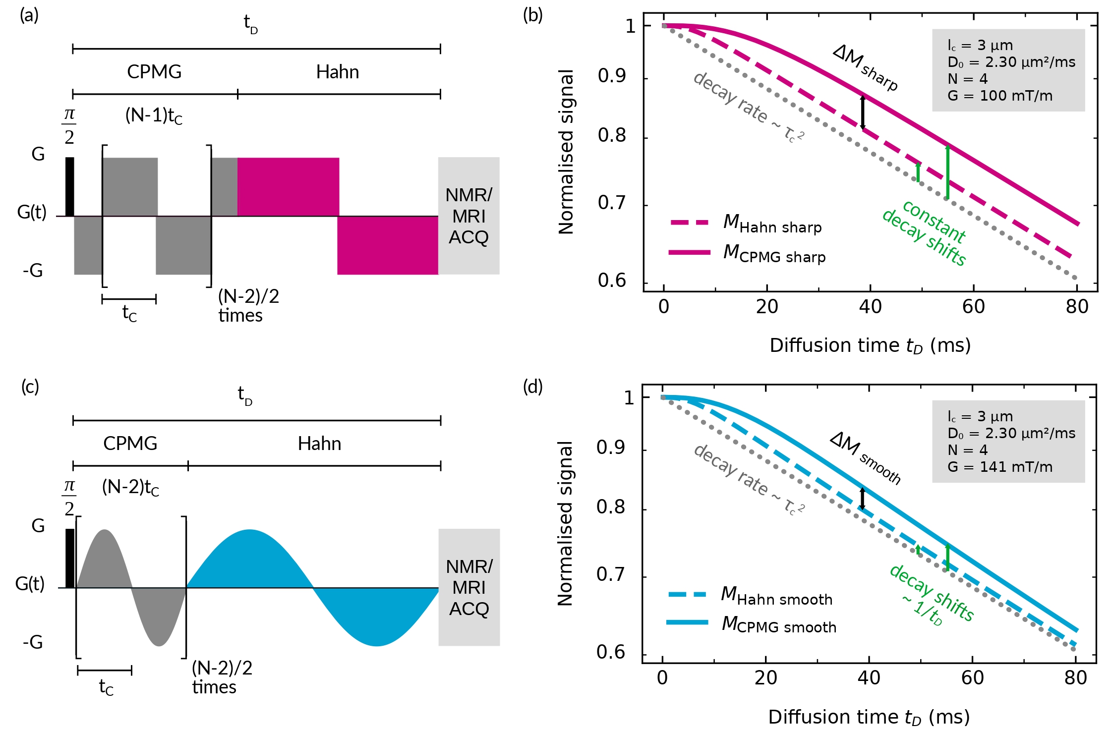
The NOGSE sequence shemesh_measuring_2013 ; alvarez_coherent_2013 is depicted in Figure 1a, schematized with a sharp modulation, i.e. with instantaneous switching of the gradient’s sign. It comprises two concatenated sequences that produce a signal decay similar to that of a CPMG (OGSE) modulation carr_effects_1954 ; meiboom_modified_1958 followed by a Hahn (Gradient Echo) modulation hahn_spin_1950 . The total diffusion time is and the total number of gradient lobes is . For the sharp gradient modulation, refocusing lobes of duration are repeated times, corresponding to the CPMG modulation. Notice that, as the modulation shape is based on a cosine symmetry, the first and last gradient pulses are of duration . The last refocusing period corresponds to the Hahn counterpart with a total duration . As , and the Echo Time between the acquired images are kept fixed, gradient switching imperfections and additional relaxation effects are factored out shemesh_measuring_2013 ; alvarez_coherent_2013 .
As instantaneous switching of the modulating gradients is not experimentally achievable, we performed the experiments with trapezoidal waveforms with the fastest slew rate possible. This sets a paradigmatic sharp gradient modulation sequence, which one can approximate as an instantaneous switch of the gradient sign, if gradient ramp times are much shorter than the lobes duration . If not, they are assumed as gradient switching imperfections that are factored out by the NOGSE approach shemesh_measuring_2013 ; alvarez_coherent_2013 .
II.4 NOGSE decay-shift for sharp modulations
The NOGSE sequence selectively probes microstructure compartment sizes from a signal decay-shift, rather than from a signal decay-rate shemesh_measuring_2013 ; alvarez_coherent_2013 ; shemesh_size_2015 ; capiglioni_noninvasive_2021 . Figure 1b shows the signal decay of the sharp-modulated NOGSE at the limiting values of the lobe duration , = for = 0 and = for = . Analysing the magnetisation signal as a function of the diffusion time , the NOGSE contrast is determined from the signal difference between the magnetisation decay at at the limiting values of , described above. The difference between these two limiting values is the NOGSE modulation contrast = .
In the restricted diffusion regime, the diffusing spins experience a spatial restriction imposed by the confining cavity. To sense these restrictions, the lobe duration needs to be longer than the restriction correlation time . At = 0 the NOGSE signal decays with the attenuation factor
| (6) |
while at , with
| (7) |
Therefore, the NOGSE contrast with a sharp gradient modulation at the diffusion restricted regime is (see Appendix A.1) shemesh_measuring_2013 ; alvarez_coherent_2013 ; capiglioni_noninvasive_2021
| (8) |
This signal evolution evidences a decay-rate that is independent of the number of lobes and it is proportional to , as in OGSE-type experiments klauder_spectral_1962 ; stepisnik_time-dependent_1993 ; callaghan_frequency-domain_1995 ; baron_oscillating_2014 ; drobnjak_pgse_2016 . The signal behaviour manifests a decay-shift, which is a constant term independent of the total diffusion time and varies as shemesh_measuring_2013 ; alvarez_coherent_2013 . This NOGSE decay-shift arises if the gradient modulations are sharp, with a parametric sensitivity to microstructure compartment sizes proportional to , enabling selective probing of specific restriction sizes capiglioni_noninvasive_2021 .
II.5 NOGSE decay-shift for smooth modulations
The NOGSE contrast of Equation 8 results from considering ideal gradient pulses, with instantaneous ramps for the switching of the applied gradient amplitude (Figure 1a). We define this case as the sharp gradient modulation that gives a decay-shift independent of the diffusion time . However, we observe that if we deviate from the ideal case scenario, i.e. if ramps are smooth (Figure 1c), the decay-shift decreases as a function of (see Figure 1d). In this study we consider for smooth gradient modulations the paradigmatic case of a sinusoidal functional dependence. Here, the first lobes, with , correspond to the CPMG modulation and the last two to the Hahn modulation, with a duration .
In order to make both implementations of NOGSE modulations comparable in the scanner, , , and take the same acquisition parameters for both types of gradient modulations.
The attenuation factor for this smooth NOGSE version at the restricted diffusion regime is (see Appendix A.2)
| (9) |
for the Hahn modulation at the limiting value and
| (10) |
for the CPMG modulation at the limiting value . Therefore, for the smooth gradient modulation, the NOGSE contrast is
| (11) |
Here, the smooth modulation evidences a parametric sensitivity to probe compartment sizes proportional to . However, the shift decays as a function of the diffusion time as a power law proportional to . This indicates that at very long diffusion times , the decay-shift might become non-observable.
III Methods
III.1 Phantom manufacturing
We mimic axon bundles with phantoms comprising aramid fibres of 12 m mean diameter. A Scanning electron microscope (SEM) image of the fibres is shown in Figure 2a and a histogram to determine their diameter distribution is shown in Figure 2b. The samples for the SEM were placed on a sample holder and glued on a carbon tape. Subsequently, the sample holder was placed in a gold bath for one minute, generating a gold layer of approximately 10 nm.
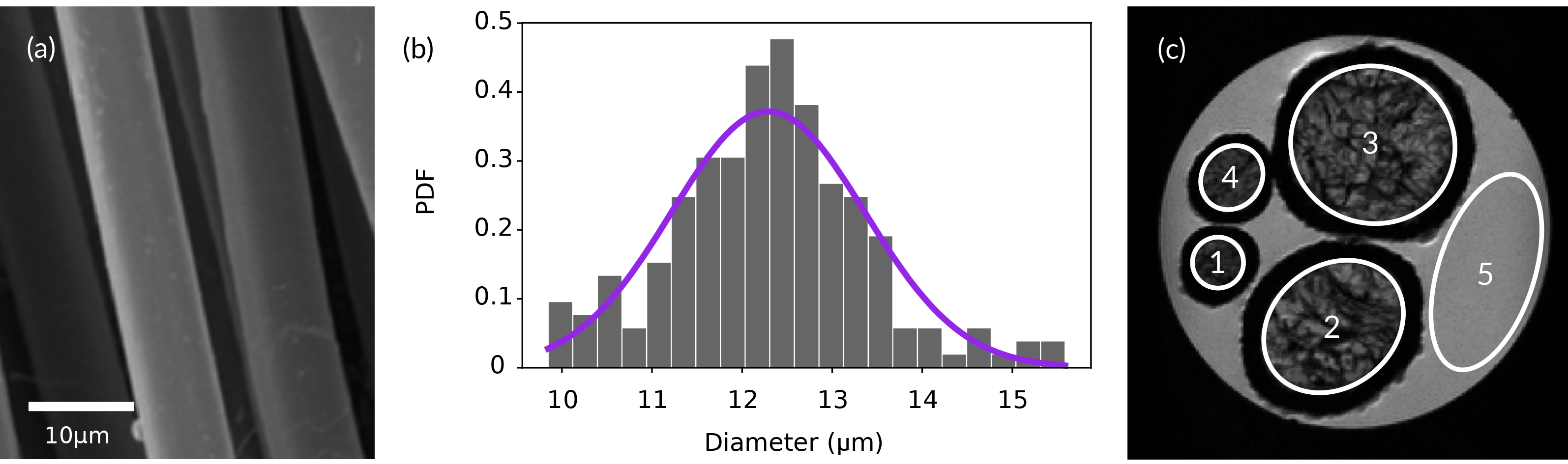
To prepare the phantoms, fibres were aligned together and positioned inside a thermo-shrinkable plastic tube to form a fibre bundle. Then, it was heated to enhance the compaction degree. Several fibre bundles were put into a 15 ml conical centrifuge tube, and then they were slowly filled with demineralized water so as to let the water enter the fibre bundles by capillary effect. Once the phantom was completely immersed in water, it was left in ultrasound to remove the remaining air bubbles.
As the fibres are both solid and impermeable, the water diffuses within the interstices of the extra-fibre region. The presence of fibres provides a tortuous environment with displacement restrictions for the diffusing water molecules, mimicking the extra-axonal space in white matter tracts.
A transverse plane DWI of the phantom is shown in Figure 2c, where parallel aramid fibre bundles of different packing densities are shown. We define several regions-of-interest (ROIs) on the transversal plane to evaluate the microstructure restriction-size distribution of the interstitial compartments. Outside the fibre bundles in the phantom (ROI5), there is freely diffusing water that is used for calibration, control purposes and to determine the free diffusion coefficient.
III.2 Image acquisition and data processing
MRI scans were performed at 9.4T on a Bruker Avance III HD WB NMR scanner with a 1H resonance frequency of = 400.15 MHz. We used a Bruker Micro 2.5 probe capable of producing gradients of up to 1500 mT/m in the three spatial directions. We programmed and implemented with ParaVision 6 the NOGSE MRI sequences shown in Figure 3 capiglioni_noninvasive_2021 . All experiments have the following sequence parameters: the Repetition time TR = 2000 ms; Field of view (FOV) = 1616 mm2, with a matrix size of 192192, leading to an in-plane resolution of 8383 m2; and slice thickness of 1 mm.
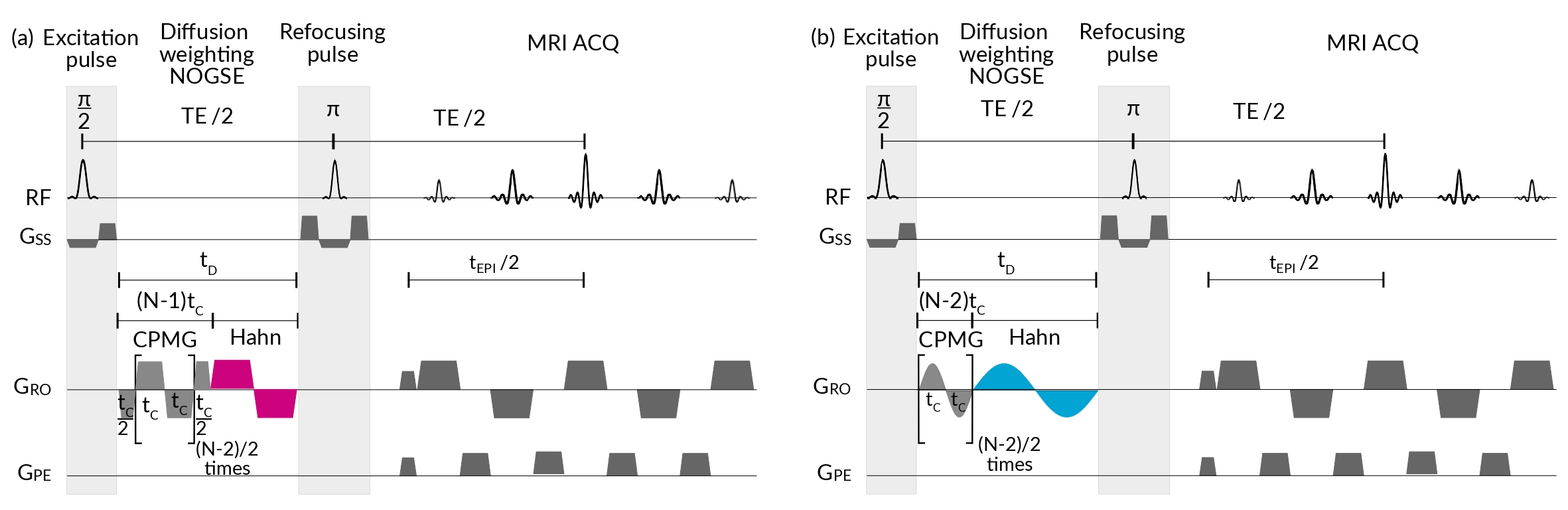
For experiments involving the analysis of the NOGSE signal vs the duration in Sections IV.2 and IV.4, the images were acquired using echo planar imaging (EPI) encoding with 4 segments with a scan time of 4 minutes with 16 averages and an echo time TE = 70.5 ms; a diffusion time varying from 12.5 ms to 24.5 ms, although in most experiments was fixed at 21.5 ms. We used for sharp modulations and for smooth modulations. The time for the lobes duration varied between 0.3 ms and ; the gradient strength varied from 20 mT/m to 600 mT/m, with ramp times of 50 mT/m/us, and were applied perpendicular to the main axis of the aramid fibre bundles.
For experiments involving the analysis of the NOGSE signal vs the diffusion time (Section IV.3), the images were acquired with an EPI encoding with 4 segments, with an image scan time of 2.5 hours with 512 averages and an echo time TE = 171.5 ms; a diffusion time varied from 1.5 ms to 80 ms. We used = 4 for sharp and smooth modulations. The lobe duration = 0.3 ms was the shortest time used to approximate the Hahn-limit modulation for NOGSE and = for the CPMG-limit NOGSE modulation. The gradient strength was = 100 mT/m and = 141 mT/m for the sharp and smooth gradient modulations, respectively, with ramp times of 50 mT/m/us. These values were chosen to make the signal decay rate in the restricted diffusion regime equal (see Equations 6 and 9). The gradients were applied perpendicular to the main axis of the aramid fibre bundles.
We determined the relaxation times = 1794.5 ms, = 70.41 ms, and = 16.294 ms in ROI1 using RARE-VTR, MSME and MGE sequences, respectively. The free water relaxation times were determined from ROI5, giving = 3409.4 ms, = 154.4 ms, = 55.181 ms.
The NOGSE signal arising from each voxel and ROI of the acquired images was analysed and plotted as a function of the NOGSE’s acquisition parameters , , or . Fittings to the experimental data were done based on the NOGSE theoretical model considering Equation 5 with the microstructure size parameters that describe the distribution, i.e. the mean size and standard deviation . A uniform free diffusion coefficient = 2.30 m2/ms of water molecules at room temperature 25 °C was used based on its experimental estimation using the signal arising from ROI5 (see Section IV.2).
III.3 NOGSE sensitivity to microstructure-size estimates
To evaluate the optimal acquisition setup for estimating microstructure restriction-size distributions, we use an information gain metric jimenez_optimization_2023 . It is the derivative of the mean square distance of the NOGSE curve with respect to changes in the parameters to be estimated, as these are obtained by fitting a theoretical representation to the experimental data based on reducing the mean square distance between the corresponding points. The highest derivative predicts the optimal NOGSE acquisition parameters for a given size distribution, consistently with quantum information estimation bounds zwick_precision_2020 ; jimenez_optimization_2023 .
More precisely, the measured magnetisation signal is defined by the acquisition parameters and the parameters that characterise the underlying lognormal restricton-size distribution of the sample under study, (see Equation 4). Thus, the aim is to find an optimal set of parameters to measure with the greatest precision possible.
We can define the information gain metric as the sensitivity of the result of a measurement against perturbations in the real parameters to be measured .
The optimal acquisition parameters are those that maximise the distance for small variations in the vicinity of the true values . This distance is the canonical distance for Lebesgue square-integrable functions (L2), since we consider the signal measurement as a function of the gradient-lobe duration , and it is given by
| (12) |
As we aim to optimise two acquisition parameters – the diffusion time and gradient strength – we define the information gain metric
| (13) |
as the mean of the distance over an ellipsoidal curve , which is given by
| (14) |
This curve parametrises an ellipse with minor and major radius and . The parameter defines the over which the distance will be calculated. The minimum value corresponds to taking and the maximum value , to and .
In this way, we obtain the sensitivity of the result of a measurement to changes in the set of parameters as a function of . Therefore, the optimal control parameters will be those that maximise this information gain metric .
relaxation was included in the calculation of the information gain metric assuming ideal modulations of the NOGSE sequences and echo time , without accounting for the noise introduced on the signal acquisition process. The echo time was calculated as = + , with being the time left for the RF pulses and crusher gradients. The maximum diffusion time considered was .
IV Results and Discussion
IV.1 Optimising Acquisition Parameters for Accurate Estimation of Restriction-Size Distributions
We first performed a preliminary estimation of the restriction size distribution in ROI1 of the fibre phantom (Figure 2c) to determine the NOGSE optimal configuration using the method described in Section III.3. We obtained = 7.3 m and = 2.8 m from a fitting of the theoretical model of Equation 5 to the experimental data. These values of and are the averaged parameters that describe the size distributions obtained using the smooth NOGSE modulation, with = 16, and several measasurements performed within the diffusuon time and gradinet strength ranges 40 - 60 ms and 70 - 300 mT/m, respectively. They were used as reference values to predict the optimal values of , and the NOGSE diffusion time for each type of gradient modulation using the protocol described in Section III.3.
According to previous works, the number of refocusing periods should be kept to a minimum for a better inference of the microstructure-size restriction parameter zwick_precision_2020 . We found consistent results in the numerical evaluation; therefore, we kept the number of refocusing periods at the lowest achievable value. According to the available NOGSE modulation sequence design (Figure 1), the lowest used are 2 and 4 for the sharp and smooth gradient modulation, respectively.
Then, we performed a systematic exploration of the information gain metric described in Section III.3, as a function of and . Figure 4 shows three information gain maps for the NOGSE modulations with = 2 or = 4 and = 4, respectively. They show the optimal values of the acquisition parameters and to estimate the restriction size distribution, corresponding to the highest information gain. For the NOGSE sharp modulation: = 35.9 ms and = 94.6 mT/m for = 2, and = 37 ms and = 99.5 mT/m for = 4. Whereas for the NOGSE smooth modulation: = 35.2 ms and = 144.3 mT/m. Although we find the optimal diffusion time around 36 ms, we used a lower value to improve signal-to-noise ratio (SNR) in all images. By experimental observation, we found = 21.5 ms to have a good compromise between the predicted optimal value and the SNR of the images.
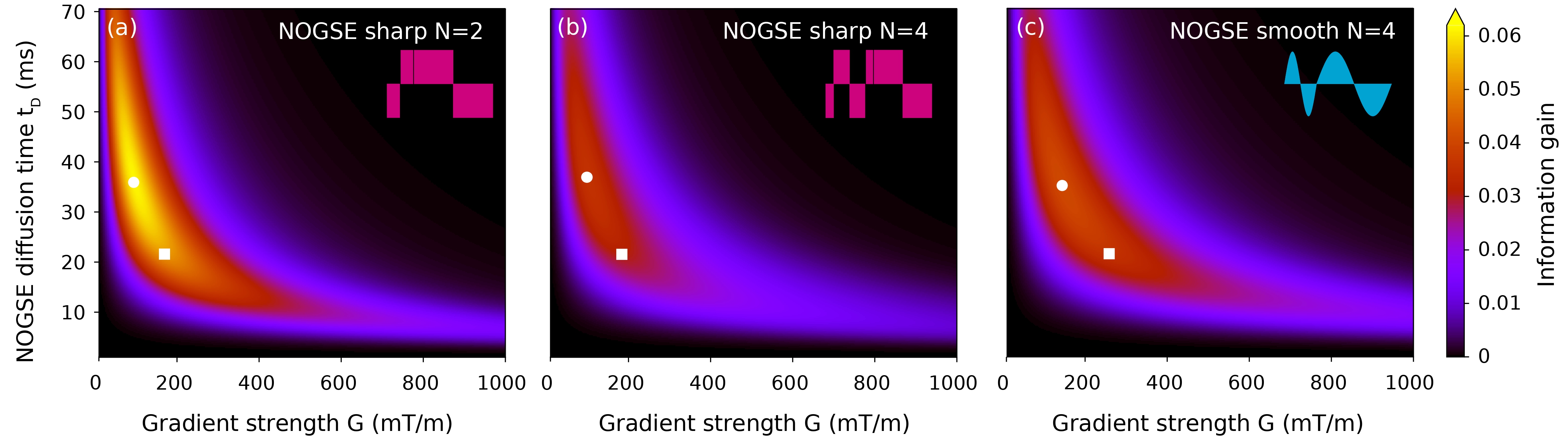
At = 21.5 ms, the predicted optimal gradient strengths for the sharp modulations are = 169 mT/m with = 2 and = 184 mT/m if = 4, and for the smooth modulation = 259 mT/m with = 4. As evidenced in Figure 4, there is a plateau on the information gain where NOGSE reaches a comparable information gain (yellow-red region). Hence, we expect a similar estimation accuracy of the underlying microstructure size distribution by choosing and within this region. Furthermore, we do not find a significant difference between using sharp or smooth modulations. However, the required gradient strength increases for the smooth modulations, and gives a slightly better precision.
IV.2 Estimation of the free diffusion coefficient
We estimate the free diffusion coefficient based on the free water signal in ROI5 (Figure 2c). When the diffusion time is much shorter than , we achieve the free diffusion limit. The NOGSE magnetisation decays with the attenuation factor
| (15) |
for the sharp gradient modulation and
| (16) |
for the smooth NOGSE modulation. Notice that both expressions are independent of , and consequently, of the restriction size . We use these expressions to estimate . Figure 5 shows the estimated values as a function of the NOGSE acquisition parameters , and , for the smooth and sharp modulations.
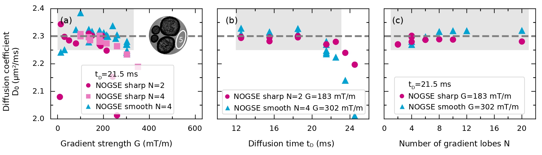
Figure 5 demonstrates that there is a range for the values of the acquisition parameters , and where the estimated remains stable around = (2.30 0.03) m2/ms (averaged value of all the experiments performed in the shaded regions of the figure). These regions are thus more sensitive for accurately estimating .
Outside of these regions, for gradient strengths exceeding approximately 300 mT/m, the signal experiences low SNR, resulting in an inefficient estimation. Similarly, excessively long diffusion times reduce SNR, leading to a diminished estimation efficiency. In contrast, for very low gradient strengths, selective RF pulses and image encoding introduce diffusion weighting effects, eclipsing the NOGSE diffusion weighting. The variation of the number of gradient lobes within the explored dynamic range does not yield significant changes. Nonetheless, a slight improvement is observed by increasing .
We use the estimated free diffusion coefficient = 2.30 m2/ms to obtain the restriction size distributions present in the different aramid fibre bundles of the phantom. Notice that the optimal acquisition parameters to estimate restriction size distributions are not in general the same as those identified for estimating . For instance, an optimal diffusion time to sense restriction size distributions needs to be long enough to allow water molecules to fully explore the compartment restrictions zwick_precision_2020 . On the contrary, the optimal inference of the free diffusion coefficient does not require the water molecules to sense the compartment confinement.
IV.3 Validating NOGSE decay-shift predictions: a proof of concept
We experimentally assess the manifestation of the NOGSE decay-shift by applying both gradient modulations on the white-matter phantom. Figure 6a displays the experimental measurements of the NOGSE signal decay, depicted in pink for the sharp modulation and light blue for the smooth modulation. The NOGSE decay is shown for the limiting values of (Hahn modulation, triangles) and = (CPMG modulation, circles) with = 4 as a function of the total diffusion time , for both sharp and smooth gradient modulations.
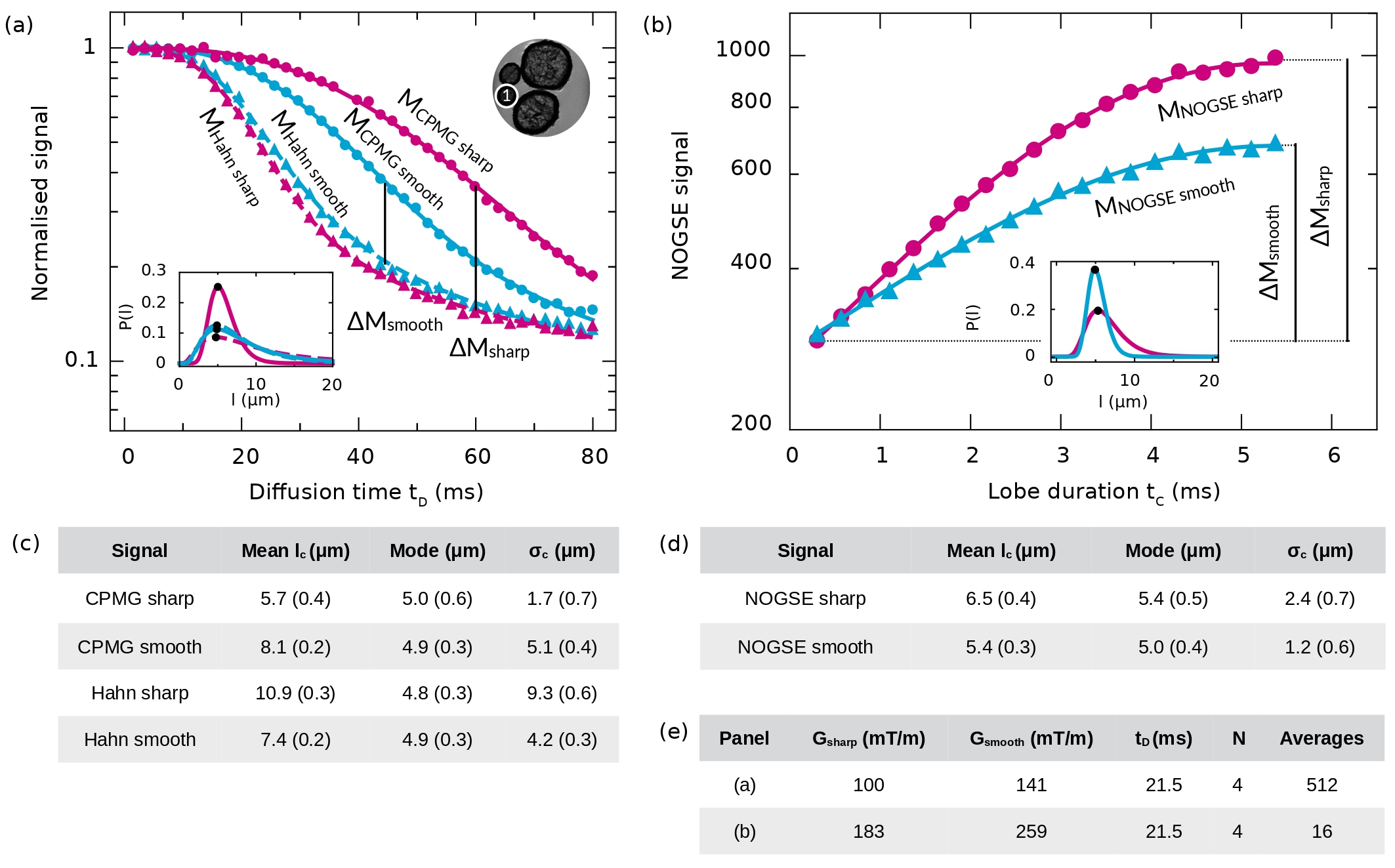
The selected acquisition parameters for the NOGSE sequence setup ensure that both modulations yield the same decay rate within the restricted diffusion regime for a single restriction size. Based on Equations 8 and 11, this condition is achieved when = . Hence, we chose = 100 mT/m and = 141 mT/m as in Figures 1b and d.
Comparing the signal decays shown in Figure 6a with the ones predicted by the theoretical model for a single restriction size in Figures 1b and d, we find that the overall behaviour of the predicted shifts is observed. The main difference is due to the restriction size distribution effects on the experimental data regardless of the chosen modulation type. Each restriction size from the probability distribution modelled by Equation 5, contributes with a different decay rate and shift, which are manifested differently as a function of the diffusion time . Still, in the region of the normalised signal within 0.3 and 0.6 an effective restriction size seems to dominate on the decaying curve manifesting the expected shift of the exponentially decaying curves as in Figures 1b and d. At longer times, the spin signal contribution from smaller restrictions becomes dominant and the decaying laws change. Moreover, Rician noise effects may also become significant.
The NOGSE signal shift reduces as a function of the diffusion time significantly faster for the smooth modulation compared with the sharp modulation as expected. For the sharp modulation, it also seems to be reduced. In this latter case, it might be due to the fact that the sharp modulations are performed with trapezoidal pulse gradients, which are not instantaneous as in the theoretical model. It might also be due to the size-distribution effects or Rician noise manifestation.
The fit of the theoretical representations to the experimental data provides comparable size distributions for both types of gradient modulations. The modes of the distributions are shown with black dots which are indistinguishable between the different cases. However, the distribution width evidences some variations (see the caption of Figure 6). We provide further discussions about these differences in the following section.
We also present the NOGSE signal as a function of the lobe duration in Figure 6b. As predicted, the NOGSE contrast is larger for the sharp modulation. As shown in the inset, the extracted size distributions from the fitting of the theoretical model of Equation 5 to the experimental data are also comparable. Again, the mode is robust, i.e. they are indistinguishable in both cases, yet there are differences on the distribution widths.
IV.4 Estimation of restriction-size distributions
We performed a more systematic evaluation of the reconstructed restriction size distributions determined from the different NOGSE sequences using sharp and smooth gradient modulations. We carried out NOGSE experiments for different , and as a function of the lobe duration , as shown in Figure 6b. Figure 7 shows the extracted parameters that characterise the corresponding estimated size distributions for all the considered cases. We present the mode, median, mean size and standard deviation of the restriction size distribution obtained from the fitted curves to the experimental data of the averaged signal of ROI1. The symbols represent the fitted size distribution parameters as a function of different NOGSE modulations and acquisition parameters: (Figure 7a), (Figure 7b) and (Figure 7c).
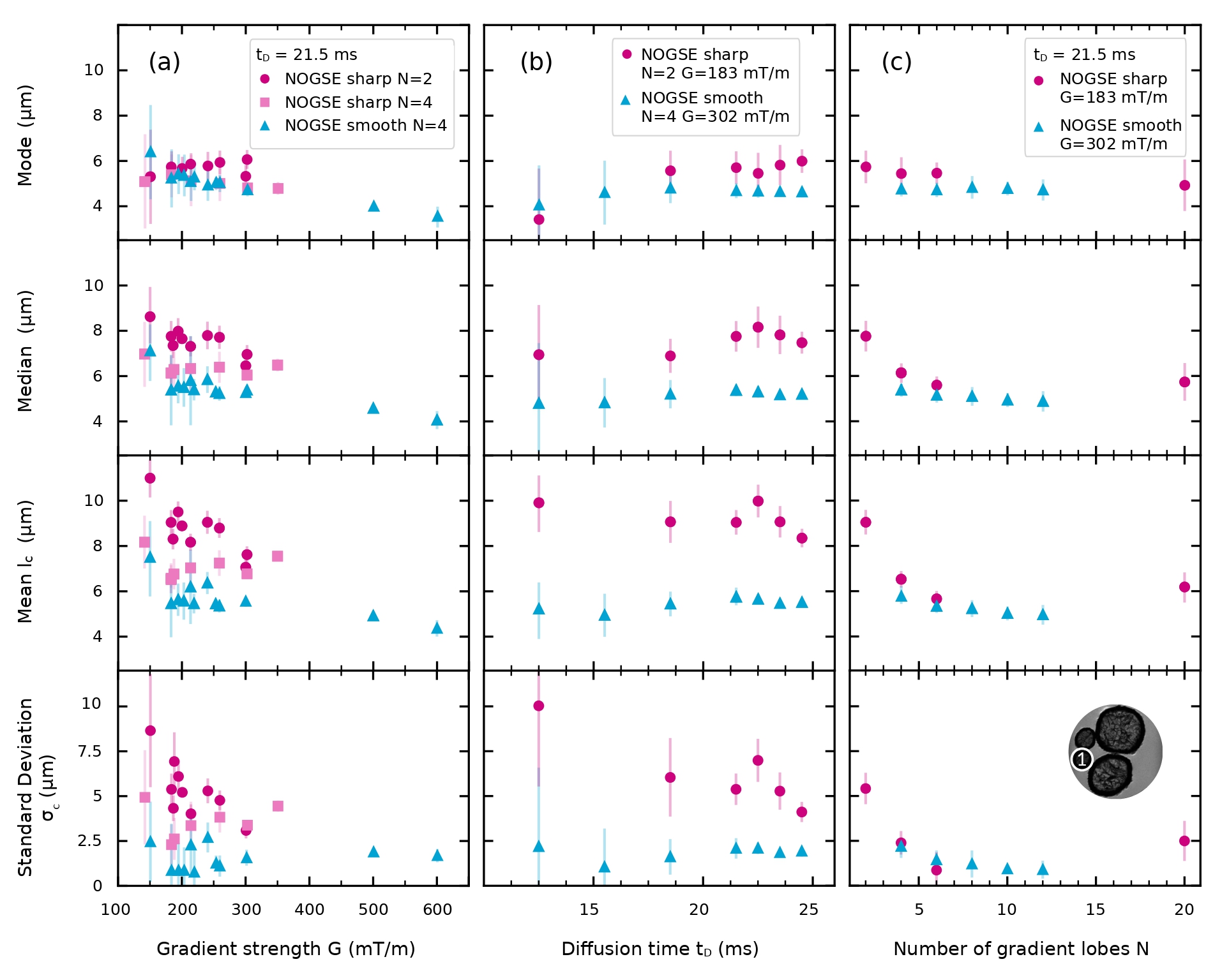
For both modulation types, the mean size and standard deviation have more dispersion than the mode and, in second place, than the median. The mode evidences to be a more robust parameter for characterising the restriction-size compared to the mean size. For all the cases, including variations of , and , the mode is quite stable near to the optimal setup parameters of the sequence for the restriction-size inference predicted in Section IV.1. It is even robust when comparing the different modulation shapes of the gradient. However, the mean and median sizes do not manifest robustness, as they are dependent on the value of the estimated standard deviation .
As the sequence is not sensitive to sizes larger than those explored during the diffusion time, the estimation of size distributions appears to incline towards a distribution that encompasses larger sizes beyond the range of exploration due to the lack of sensitivity to them. The estimation of larger sizes is correlated with the inclusion of smaller sizes when increasing . For this reason, despite the dispersion of the distribution shape, the mode seems always to be a robust parameter to characterise the system.
Both NOGSE modulations estimate similar lognormal distributions, although we find that, in general, smooth gradient modulations give slightly smaller microstructure-size mode and mean values, as well as for the distribution widths. Similar qualitative behaviours are observed for the extracted size distribution parameter from different ROIs in the phantom.
The estimated values have less dispersion when estimated with NOGSE acquisition parameters near to the optimal region predicted in Section IV.1. Notice that higher parametric fluctuations are observed at the lower and higher ends of the gradient strengths and also at the extremes of the explored range for the diffusion time. These extremes are less sensitive for estimating the size distribution parameters as they are far from the optimal setup for the inference. We find, in general, that the regions with less dispersion in the estimated size distribution parameters, are at a bit higher gradient strengths compared with the predicted optimal value. In particular this is more noticeable for the sharp modulation. This seems to be consistent with the fact that the numerical predictions assume ideal squared shapes, while in practice they have trapezoidal shapes. By increasing , we find that the estimation provides slightly lower restriction sizes. This is consistent with the fact that the lower possible is the most sensitive for estimating restriction sizes zwick_precision_2020 and that increasing for the same diffusion time reduces the maximum restriction sizes that can be estimated.
In addition to evaluate the consistency of the estimations, we compare the resulting restriction size distributions obtained from the averaged signal of a ROI as shown in Figure 7 with the ones obtained from single-restriction size fits from the voxel-by-voxel data. In this case, we use the NOGSE parameters derived from the region in Figure 7a that exhibits the lowest dispersion of the estimated values. Figure 8a,b are maps of the determined single-restriction sizes for each voxel, for the sharp and smooth NOGSE modulations, respectively. The observed variations in fibre densities, based on the restriction size estimation, are consistent with the level of compaction achieved during the phantom preparation process. Notice that the assumption here is that the size-distribution width at every voxel is negligible.
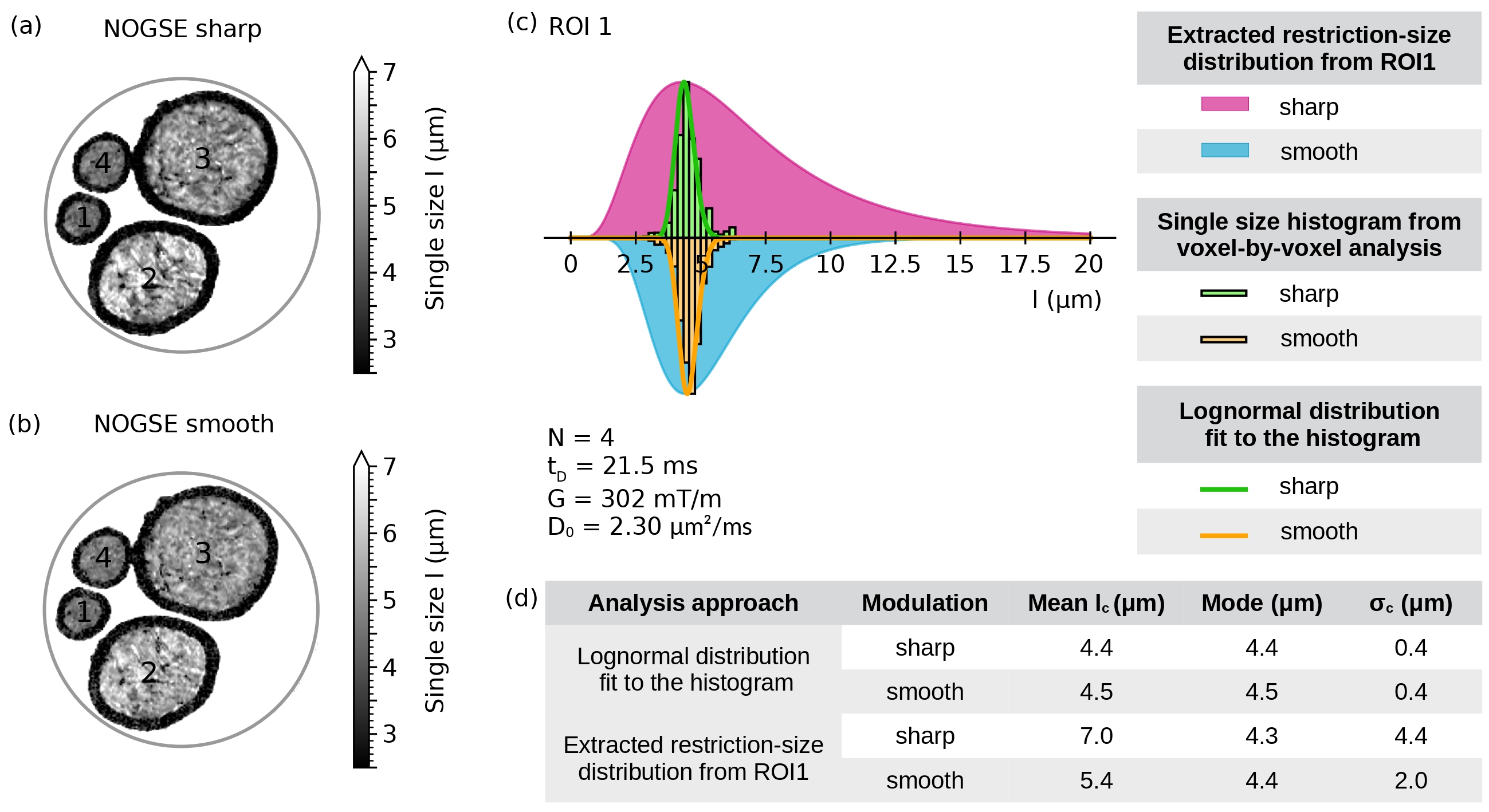
Single-size histograms from the voxel-by-voxel fits of ROI1 are shown in Figure 8c. Smooth and sharp modulations provide very similar size distributions. We also compare each histogram with the restriction-size distribution that arises from the averaged-signal fit of ROI1, for both types of gradient modulation. The distribution from the voxel-by-voxel differs from the one obtained via the averaged-signal. The distribution size mode is robust as both approaches give indistinguishable values. Nevertheless, there is an inconsistency in the distribution-width determination.
V Conclusions
Motivated by the need for improved diagnostic tools in neurodegenerative diseases, particularly in those associated with white-matter alterations, our study is focused on determining microstructural sizes using the NOGSE sequence in DWI. NOGSE has shown to be a tool to selectively probe microstructure sizes based on a decay-shift, especially using sharp gradient modulations. Our research aimed to evaluate the applicability of this technique focusing on comparing the estimation of microstructure size-distributions using both sharp and smooth gradient modulations, where the latter is more suitable for clinical protocols.
For this purpose we designed home-made phantoms to mimic axon bundles, in particular to study the diffusion within the extra-axonal compartments. We demonstrated with a combination of analytical derivations and numerical simulations using information theory tools, contrasted with proof-of-principle experiments, that both modulations can be used to estimate restriction-size distributions using NOGSE and its decay-shift. We found that both types of modulation give comparable microstructural information.
By a systematic analysis of the estimated microstructural properties of the white-matter phantom, we evaluate the reliability and self-consistency of obtaining compartment-size distributions with the NOGSE sequence. We found that the estimation of the distribution’s mode is very robust, and thus reliable for both, sharp and smooth gradient modulations. On the contrary, the mean, median size and its distribution width are less robust. While further work needs to be performed, this seems to be associated with indistinguishable properties of the assumed log-normal distribution than to a specific method for the inference.
Overall, the presented results are a step towards improving diagnostic tools based on quantitative imaging of tissue microstructure that might allow early stage diagnosis of neurodegenerative diseases associated with axon alterations in the white matter of the brain.
Acknowledgements
This work was supported by CNEA; CONICET, ANPCyT-FONCyT PICT-2017-3156, PICT-2017-3699, PICT-2018-4333, PICT-2021-GRF-TI-00134, PICT-2021-I-A-00070; PIP-CONICET (11220170100486CO); UNCUYO SIIP Tipo I 2019-C028, 2022-C002, 2022-C030; Instituto Balseiro; Collaboration programs between the MINCyT (Argentina) and, MAECI (Italy) and MOST (Israel); and Erasmus+ Higher Education program from the European Commission between the CIMEC (University of Trento) and the Instituto Balseiro (Universidad Nacional de Cuyo).
*
Appendix A NOGSE magnetisation decay
As mentioned in the Theory section of the main text (Subsection II.1), the magnetisation signal observed from an ensemble of non-interacting and equivalent spins under the effects of a modulated gradient sequence is = . Here, = is the phase acquired by a spin during the evolution time , and the brackets denote the average over the random phases of the spin ensemble hahn_spin_1950 ; carr_effects_1954 . For the considered modulated gradient spin-echo sequences, the average phase becomes = 0. Then, as typically follows a Gaussian distribution klauder_spectral_1962 ; stepisnik_analysis_1981 ; stepisnik_validity_1999 , the signal will evidence a decay depending on the random phase variance as
| (17) |
The attenuation factor can be written in a Fourier representation as stepisnik_time-dependent_1993 ; lasic_displacement_2006 ; shemesh_measuring_2013 ; alvarez_coherent_2013 ; zwick_maximizing_2016
| (18) |
Within this FT representation, the signal decay is determined by the integral of the overlap between the filter function and the spectral density . The filter only depends on the setup parameters of the chosen MGSE sequence, since it is defined by the FT of the gradient modulation . The spectral density only depends on the characteristics of the diffusion-driven fluctuations, given by
| (19) |
where is the free diffusion coefficient and is the time required for most molecules to fully probe the compartment boundaries. Considering the Einstein’s expression = , the characteristic time is related to the restriction length of the microstructure compartment in which diffusion is taking place callaghan_translational_2011 . Therefore, by suitably choosing the oscillating gradient modulation parameters to steer the NMR signal decay, one can probe the water diffusion process and, consequently, extract microstructural restriction sizes from its time dependence gore_characterization_2010 ; shemesh_measuring_2013 ; alvarez_coherent_2013 ; capiglioni_noninvasive_2021 .
In the following Subsections we specify the signal decays expressions for the sharp and smooth gradient modulations used in this work (see Figures 1a and c for a single diffusion restriction size ).
A.1 NOGSE signal decay for sharp gradient modulations
For the ideal NOGSE sequence shown in Figure 1a of the main text, gradient lobes of duration are repeated with alternated sign times giving the CPMG modulation and a last refocusing period which corresponds to the Hahn counterpart. The total diffusion duration for the CPMG part is and for the Hahn part, . For the sharp gradient modulation, the NOGSE magnetisation decay is shemesh_measuring_2013 ; alvarez_coherent_2013
| (20) |
with the Hahn signal decay given by
| (21) |
and for the CPMG signal decay by
| (22) |
with
| (23) |
and
| (24) |
The cross term has an argument
| (25) |
The difference between the two limiting values, and of this expression is the NOGSE sharp modulation contrast .
When the diffusion times and are much longer than , the NOGSE magnetisation decay in the restricted diffusion regime is
| (26) |
from which we obtain the restricted diffusion expressions for the Hahn modulation at the limiting value and for the CPMG modulation at = (Equations 6 and 7, respectively). With these expressions we obtain the NOGSE contrast from Equation 8.
In the free diffusion regime, where the diffusion times are much shorter than , the NOGSE magnetisation decays with
| (27) |
A.2 NOGSE signal decay for smooth gradient modulations
Instead, if we consider a sinusoidal waveform as a representation of a smooth gradient modulation as in Figure 1c, the NOGSE sharp magnetisation decay for a given restriction size results
| (28) |
The Hahn modulation for the smooth gradient modulation has a duration of = . The difference between the two limiting values, and = from this expression is the NOGSE smooth modulation contrast .
When considering the restricted diffusion regime, the NOGSE magnetisation decay in this case results
| (29) |
from which we obtain the restricted diffusion expressions for the Hahn and CPMG extremes of Equations 9 and 10, respectively, yelding the NOGSE contrast from Equation 11.
In the free diffusion regime, the NOGSE smooth magnetisation decays with
| (30) |
References
- (1) De Santis S, Gabrielli A, Palombo M, Maraviglia B, Capuani S. Non-Gaussian diffusion imaging: a brief practical review. Magnetic Resonance Imaging. 2011;29(10):1410-1416. Proceedings of the International School on Magnetic Resonance and Brain Functiondoi: https://doi.org/10.1016/j.mri.2011.04.006
- (2) White NS, Leergaard TB, D’Arceuil H, Bjaalie JG, Dale AM. Probing tissue microstructure with restriction spectrum imaging: Histological and theoretical validation. Human Brain Mapping. 2013;34(2):327–346. doi: 10.1002/hbm.21454
- (3) White NS, McDonald CR, Farid N, et al. Diffusion-Weighted Imaging in Cancer: Physical Foundations and Applications of Restriction Spectrum Imaging. Cancer Research. 2014;74(17):4638–4652. doi: 10.1158/0008-5472.CAN-13-3534
- (4) Alexander DC, Dyrby TB, Nilsson M, Zhang H. Imaging brain microstructure with diffusion MRI: practicality and applications. NMR in Biomedicine. 2019;32(4):e3841. doi: 10.1002/nbm.3841
- (5) Xu J, Jiang X, Li H, et al. Magnetic resonance imaging of mean cell size in human breast tumors. Magnetic Resonance in Medicine. 2020;83(6):2002-2014. doi: 10.1002/mrm.28056
- (6) Fokkinga E, Hernandez-Tamames JA, Ianus A, et al. Advanced Diffusion-Weighted MRI for Cancer Microstructure Assessment in Body Imaging, and Its Relationship With Histology. J. Magn. Reson. Imaging. 2023;n/a(n/a). doi: https://doi.org/10.1002/jmri.29144
- (7) Le Bihan D. Looking into the functional architecture of the brain with diffusion MRI. Nat Rev Neurosci. 2003;4(6):469–480. doi: 10.1038/nrn1119
- (8) Xu J, Li H, Harkins KD, et al. Mapping mean axon diameter and axonal volume fraction by MRI using temporal diffusion spectroscopy. NeuroImage. 2014;103:10–19. doi: 10.1016/j.neuroimage.2014.09.006
- (9) Jack Jr. CR, Bernstein MA, Fox NC, et al. The Alzheimer’s disease neuroimaging initiative (ADNI): MRI methods. Journal of Magnetic Resonance Imaging. 2008;27(4):685-691. doi: https://doi.org/10.1002/jmri.21049
- (10) Drago V, Babiloni C, Bartrés-Faz D, et al. Disease Tracking Markers for Alzheimer’s Disease at the Prodromal (MCI) Stage. Journal of Alzheimer’s Disease. 2011;26(s3):159–199. doi: 10.3233/JAD-2011-0043
- (11) Harrison JR, Bhatia S, Tan ZX, et al. Imaging Alzheimer’s genetic risk using diffusion MRI: A systematic review. NeuroImage: Clinical. 2020;27:102359. doi: https://doi.org/10.1016/j.nicl.2020.102359
- (12) Chu X, Wu P, Yan H, et al. Comparison of brain microstructure alterations on diffusion kurtosis imaging among Alzheimer’s disease, mild cognitive impairment, and cognitively normal individuals. Front. aging neurosci.. 2022;14:919143.
- (13) Hyde KL, Samson F, Evans AC, Mottron L. Neuroanatomical differences in brain areas implicated in perceptual and other core features of autism revealed by cortical thickness analysis and voxel-based morphometry. Hum Brain Mapp. 2010;31(4):556–566. doi: 10.1002/hbm.20887
- (14) Enzinger C, Barkhof F, Ciccarelli O, et al. Nonconventional MRI and microstructural cerebral changes in multiple sclerosis. Nat Rev Neurol. 2015;11(12):676–686. doi: 10.1038/nrneurol.2015.194
- (15) Grussu F, Schneider T, Tur C, et al. Neurite dispersion: a new marker of multiple sclerosis spinal cord pathology?. Annals of Clinical and Translational Neurology. 2017;4(9):663–679. doi: 10.1002/acn3.445
- (16) Kubicki M, McCarley R, Westin CF, et al. A review of diffusion tensor imaging studies in schizophrenia. Journal of Psychiatric Research. 2007;41(1):15–30. doi: 10.1016/j.jpsychires.2005.05.005
- (17) Canazza A, Minati L, Boffano C, Parati E, Binks S. Experimental Models of Brain Ischemia: A Review of Techniques, Magnetic Resonance Imaging, and Investigational Cell-Based Therapies. Front. neurol.. 2014;5:63894.
- (18) Zhu LH, Zhang ZP, Wang FN, Cheng QH, Guo G. Diffusion kurtosis imaging of microstructural changes in brain tissue affected by acute ischemic stroke in different locations. Neural Regen Res. 2019;14(2):272–279. doi: 10.4103/1673-5374.244791
- (19) Caminiti R, Carducci F, Piervincenzi C, et al. Diameter, Length, Speed, and Conduction Delay of Callosal Axons in Macaque Monkeys and Humans: Comparing Data from Histology and Magnetic Resonance Imaging Diffusion Tractography. J. Neurosci.. 2013;33(36):14501–14511. doi: 10.1523/JNEUROSCI.0761-13.2013
- (20) Maier-Hein KH, Neher PF, Houde JC, et al. The challenge of mapping the human connectome based on diffusion tractography. Nature communications. 2017;8(1):1349.
- (21) Schilling KG, Tax CMW, Rheault F, et al. Prevalence of white matter pathways coming into a single white matter voxel orientation: The bottleneck issue in tractography. Human Brain Mapping. 2022;43(4):1196-1213. doi: https://doi.org/10.1002/hbm.25697
- (22) Maffei C, Sarubbo S, Jovicich J. Diffusion-based tractography atlas of the human acoustic radiation. Sci Rep. 2019;9(1):4046. doi: 10.1038/s41598-019-40666-8
- (23) Maffei C, Sarubbo S, Jovicich J. A Missing Connection: A Review of the Macrostructural Anatomy and Tractography of the Acoustic Radiation. Front. neuroanat.. 2019;13:27.
- (24) Huang TH, Lai MC, Chen YS, Huang CW. Brain Imaging in Epilepsy-Focus on Diffusion-Weighted Imaging. Diagnostics (Basel). 2022;12(11):2602. doi: 10.3390/diagnostics12112602
- (25) Assaf Y, Basser PJ. Composite hindered and restricted model of diffusion (CHARMED) MR imaging of the human brain. Neuroimage. 2005;27(1):48–58.
- (26) Assaf Y, Blumenfeld-Katzir T, Yovel Y, Basser PJ. Axcaliber: A method for measuring axon diameter distribution from diffusion MRI. Magnetic Resonance in Medicine. 2008;59(6):1347–1354. doi: 10.1002/mrm.21577
- (27) Patterson DM, Padhani AR, Collins DJ. Technology Insight: water diffusion MRI—a potential new biomarker of response to cancer therapy. Nat Rev Clin Oncol. 2008;5(4):220–233. doi: 10.1038/ncponc1073
- (28) Padhani AR, Liu G, Mu-Koh D, et al. Diffusion-Weighted Magnetic Resonance Imaging as a Cancer Biomarker: Consensus and Recommendations. Neoplasia. 2009;11(2):102–125. doi: 10.1593/neo.81328
- (29) Ong HH, Wehrli FW. Quantifying axon diameter and intra-cellular volume fraction in excised mouse spinal cord with q-space imaging. NeuroImage. 2010;51(4):1360–1366. doi: 10.1016/j.neuroimage.2010.03.063
- (30) Jelescu IO, Palombo M, Bagnato F, Schilling KG. Challenges for biophysical modeling of microstructure. Journal of Neuroscience Methods. 2020;344:108861. doi: https://doi.org/10.1016/j.jneumeth.2020.108861
- (31) Kakkar LS, Bennett OF, Siow B, et al. Low frequency oscillating gradient spin-echo sequences improve sensitivity to axon diameter: An experimental study in viable nerve tissue. NeuroImage. 2018;182:314–328. doi: 10.1016/j.neuroimage.2017.07.060
- (32) Veraart J, Nunes D, Rudrapatna U, et al. Noninvasive quantification of axon radii using diffusion MRI. eLife. 2020;9:e49855. doi: 10.7554/eLife.49855
- (33) Olesen JL, Østergaard L, Shemesh N, Jespersen SN. Diffusion time dependence, power-law scaling, and exchange in gray matter. NeuroImage. 2022;251:118976. doi: https://doi.org/10.1016/j.neuroimage.2022.118976
- (34) Alexander DC, Hubbard PL, Hall MG, et al. Orientationally invariant indices of axon diameter and density from diffusion MRI. Neuroimage. 2010;52(4):1374–1389. doi: 10.1016/j.neuroimage.2010.05.043
- (35) Zhang H, Schneider T, Wheeler-Kingshott CA, Alexander DC. NODDI: Practical in vivo neurite orientation dispersion and density imaging of the human brain. NeuroImage. 2012;61(4):1000–1016. doi: 10.1016/j.neuroimage.2012.03.072
- (36) Shemesh N, Álvarez GA, Frydman L. Measuring small compartment dimensions by probing diffusion dynamics via Non-uniform Oscillating-Gradient Spin-Echo (NOGSE) NMR. Journal of Magnetic Resonance. 2013;237:49–62. doi: 10.1016/j.jmr.2013.09.009
- (37) Novikov DS, Fieremans E, Jespersen SN, Kiselev VG. Quantifying brain microstructure with diffusion MRI: Theory and parameter estimation. NMR in Biomedicine. 2019;32(4):e3998. doi: 10.1002/nbm.3998
- (38) Palombo M, Ianus A, Guerreri M, et al. SANDI: A compartment-based model for non-invasive apparent soma and neurite imaging by diffusion MRI. NeuroImage. 2020;215:116835. doi: https://doi.org/10.1016/j.neuroimage.2020.116835
- (39) Capiglioni M, Zwick A, Jiménez P, Álvarez GA. Noninvasive Quantitative Imaging of Selective Microstructure Sizes via Magnetic Resonance. Phys. Rev. Appl.. 2021;15(1):014045. doi: 10.1103/PhysRevApplied.15.014045
- (40) Warner W, Palombo M, Cruz R, et al. Temporal Diffusion Ratio (TDR) for imaging restricted diffusion: Optimisation and pre-clinical demonstration. NeuroImage. 2023;269:119930. doi: 10.1016/j.neuroimage.2023.119930
- (41) Jelescu IO, Budde MD. Design and Validation of Diffusion MRI Models of White Matter. Frontiers in Physics. 2017;5.
- (42) Novikov DS, Kiselev VG, Jespersen SN. On modeling. Magnetic Resonance in Medicine. 2018;79(6):3172–3193. doi: 10.1002/mrm.27101
- (43) Afzali M, Pieciak T, Newman S, et al. The sensitivity of diffusion MRI to microstructural properties and experimental factors. Journal of Neuroscience Methods. 2021;347:108951. doi: 10.1016/j.jneumeth.2020.108951
- (44) Stepišnik J. Time-dependent self-diffusion by NMR spin-echo. Physica B: Condensed Matter. 1993;183(4):343–350. doi: 10.1016/0921-4526(93)90124-O
- (45) Callaghan PT, Stepišnik J. Frequency-Domain Analysis of Spin Motion Using Modulated-Gradient NMR. Journal of Magnetic Resonance, Series A. 1995;117(1):118–122. doi: 10.1006/jmra.1995.9959
- (46) Stepišnik J, Lasič S, Mohorič A, Serša I, Sepe A. Spectral characterization of diffusion in porous media by the modulated gradient spin echo with CPMG sequence. Journal of Magnetic Resonance. 2006;182(2):195–199. doi: 10.1016/j.jmr.2006.06.023
- (47) Callaghan PT. Translational Dynamics and Magnetic Resonance: Principles of Pulsed Gradient Spin Echo NMR. OUP Oxford, 2011.
- (48) Siow B, Drobnjak I, Chatterjee A, Lythgoe MF, Alexander DC. Estimation of pore size in a microstructure phantom using the optimised gradient waveform diffusion weighted NMR sequence. Journal of Magnetic Resonance. 2012;214:51–60. doi: 10.1016/j.jmr.2011.10.004
- (49) Álvarez GA, Shemesh N, Frydman L. Coherent Dynamical Recoupling of Diffusion-Driven Decoherence in Magnetic Resonance. Phys. Rev. Lett.. 2013;111(8):080404. doi: 10.1103/PhysRevLett.111.080404
- (50) Sjölund J, Szczepankiewicz F, Nilsson M, Topgaard D, Westin CF, Knutsson H. Constrained optimization of gradient waveforms for generalized diffusion encoding. Journal of Magnetic Resonance. 2015;261:157-168. doi: https://doi.org/10.1016/j.jmr.2015.10.012
- (51) Drobnjak I, Zhang H, Ianuş A, Kaden E, Alexander DC. PGSE, OGSE, and sensitivity to axon diameter in diffusion MRI: Insight from a simulation study. Magnetic Resonance in Medicine. 2016;75(2):688–700. doi: 10.1002/mrm.25631
- (52) Nilsson M, Lasič S, Drobnjak I, Topgaard D, Westin CF. Resolution limit of cylinder diameter estimation by diffusion MRI: The impact of gradient waveform and orientation dispersion. NMR in Biomedicine. 2017;30(7):e3711. doi: 10.1002/nbm.3711
- (53) Stepišnik J. Analysis of NMR self-diffusion measurements by a density matrix calculation. Physica B+C. 1981;104(3):350-364. doi: https://doi.org/10.1016/0378-4363(81)90182-0
- (54) Does MD, Parsons EC, Gore JC. Oscillating gradient measurements of water diffusion in normal and globally ischemic rat brain. Magnetic Resonance in Medicine. 2003;49(2):206-215. doi: https://doi.org/10.1002/mrm.10385
- (55) Gore JC, Xu J, Colvin DC, Yankeelov TE, Parsons EC, Does MD. Characterization of tissue structure at varying length scales using temporal diffusion spectroscopy. NMR in Biomedicine. 2010;23(7):745–756. doi: 10.1002/nbm.1531
- (56) Stejskal EO, Tanner JE. Spin Diffusion Measurements: Spin Echoes in the Presence of a Time-Dependent Field Gradient. J. Chem. Phys.. 1965;42(1):288–292. doi: 10.1063/1.1695690
- (57) Grebenkov DS. NMR survey of reflected Brownian motion. Rev. Mod. Phys.. 2007;79(3):1077–1137. doi: 10.1103/RevModPhys.79.1077
- (58) Smith PE, Bensky G, Álvarez GA, Kurizki G, Frydman L. Shift-driven modulations of spin-echo signals. Proceedings of the National Academy of Sciences. 2012;109(16):5958–5961. doi: https://doi.org/10.1073/pnas.1120704109
- (59) Zwick A, Álvarez GA. Quantum sensing tools to characterize physical, chemical and biological processes with magnetic resonance. Journal of Magnetic Resonance Open. 2023;16-17:100113. doi: https://doi.org/10.1016/j.jmro.2023.100113
- (60) Shemesh N, Álvarez GA, Frydman L. Size Distribution Imaging by Non-Uniform Oscillating-Gradient Spin Echo (NOGSE) MRI. PLOS ONE. 2015;10(7):e0133201. doi: 10.1371/journal.pone.0133201
- (61) Klauder JR, Anderson PW. Spectral Diffusion Decay in Spin Resonance Experiments. Phys. Rev.. 1962;125(3):912–932. doi: 10.1103/PhysRev.125.912
- (62) Stepišnik J. Analysis of NMR self-diffusion measurements by a density matrix calculation. Physica B+C. 1981;104(3):350–364. doi: 10.1016/0378-4363(81)90182-0
- (63) Stepišnik J. Validity limits of Gaussian approximation in cumulant expansion for diffusion attenuation of spin echo. Physica B: Condensed Matter. 1999;270(1):110–117. doi: 10.1016/S0921-4526(99)00160-X
- (64) Lasič S, Stepišnik J, Mohorič A. Displacement power spectrum measurement by CPMG in constant gradient. Journal of Magnetic Resonance. 2006;182(2):208–214. doi: 10.1016/j.jmr.2006.06.030
- (65) Zwick A, Álvarez GA, Kurizki G. Maximizing Information on the Environment by Dynamically Controlled Qubit Probes. Phys. Rev. Appl.. 2016;5(1):014007. doi: 10.1103/PhysRevApplied.5.014007
- (66) Zwick A, Suter D, Kurizki G, Álvarez GA. Precision Limits of Tissue Microstructure Characterization by Magnetic Resonance Imaging. Phys. Rev. Appl.. 2020;14(2):024088. doi: 10.1103/PhysRevApplied.14.024088
- (67) Barazany D, Basser PJ, Assaf Y. In vivo measurement of axon diameter distribution in the corpus callosum of rat brain. Brain. 2009;132(5):1210–1220. doi: 10.1093/brain/awp042
- (68) Nilsson M, Westen vD, Ståhlberg F, Sundgren PC, Lätt J. The role of tissue microstructure and water exchange in biophysical modelling of diffusion in white matter. Magn Reson Mater Phy. 2013;26(4):345–370. doi: 10.1007/s10334-013-0371-x
- (69) Pajevic S, Basser PJ. An Optimum Principle Predicts the Distribution of Axon Diameters in Normal White Matter. PLOS ONE. 2013;8(1):e54095. doi: 10.1371/journal.pone.0054095
- (70) Liewald D, Miller R, Logothetis N, Wagner HJ, Schüz A. Distribution of axon diameters in cortical white matter: an electron-microscopic study on three human brains and a macaque. Biol Cybern. 2014;108(5):541–557. doi: 10.1007/s00422-014-0626-2
- (71) Carr HY, Purcell EM. Effects of Diffusion on Free Precession in Nuclear Magnetic Resonance Experiments. Phys. Rev.. 1954;94(3):630–638. doi: 10.1103/PhysRev.94.630
- (72) Meiboom S, Gill D. Modified Spin-Echo Method for Measuring Nuclear Relaxation Times. Review of Scientific Instruments. 1958;29(8):688–691. doi: 10.1063/1.1716296
- (73) Hahn EL. Spin Echoes. Phys. Rev.. 1950;80(4):580–594. doi: 10.1103/PhysRev.80.580
- (74) Baron CA, Beaulieu C. Oscillating gradient spin-echo (OGSE) diffusion tensor imaging of the human brain. Magnetic Resonance in Medicine. 2014;72(3):726–736. doi: 10.1002/mrm.24987
- (75) Jimenez PJ, Zwick AE, Álvarez GA. Optimization method for estimating tissue microstructure size-distributions with diffusion weighted imaging. Proc. Intl. Soc. Mag. Reson. Med. 2023;31(4485).