Optimization of nonequilibrium free energy harvesting illustrated on bacteriorhodopsin
Abstract
Harvesting free energy from the environment is essential for the operation of many biological and artificial systems. We use techniques from stochastic thermodynamics to investigate the maximum rate of harvesting achievable by optimizing a set of reactions in a Markovian system, possibly under various kinds of topological, kinetic, and thermodynamic constraints. This question is relevant for the optimal design of new harvesting devices as well as for quantifying the efficiency of existing systems. We first demonstrate that the maximum harvesting rate can be expressed as a constrained convex optimization problem. We illustrate it on bacteriorhodopsin, a light-driven proton pump from Archaea, which we find is close to optimal under realistic conditions. In our second result, we solve the optimization problem in closed-form in three physically meaningful limiting regimes. These closed-form solutions are illustrated on two idealized models of unicyclic harvesting systems.
I Introduction
Many molecular systems, both biological and artificial, harvest free energy from their environments. Biological organisms require free energy to grow and replicate [1, 2], and many species undergo selection for increased harvesting [3, 4, 5, 6]. Artificial harvesting systems have also been constructed and optimized in the field of synthetic biology [7, 8, 9, 10, 11, 12, 13, 14]. The optimization of free energy harvesting is thus a central problem both in biology and engineering.
As an example, consider a harvesting system such as a biological metabolic network that converts glucose to ATP [15]. Suppose that the kinetic and thermodynamic parameters of one or more reactions can be optimized, either by natural selection or artificial design. What is the maximum rate of free energy harvesting that the network can achieve, and what are the kinetic and thermodynamic parameters that achieve it? These questions are relevant both for design of optimal harvesting devices and for quantifying the efficiency of existing systems.
In this paper, we use techniques from stochastic thermodynamics to derive bounds on maximum rate of free energy harvesting. We consider a harvesting system in nonequilibrium steady state which is coupled to an external source of free energy, an internal free energy reservoir, and a heat bath. The setup is well-suited for studying the kinds of small-scale systems usually considered in stochastic thermodynamics [16], where assumptions of local detailed balance and steady state are justified. The steady-state assumption is reasonable in many molecular systems, where there is a separation of timescales between internal relaxation and environmental change.
We suppose that the system’s dynamics can be separate into two kinds of processes, termed baseline and control. The baseline processes, which are held fixed, mediate the coupling to the external source of free energy. Control refers to all other processes which can be optimized for increasing the harvesting rate at which free energy flows into the internal reservoir. The particular separation of baseline/control generally depends on domain knowledge about the system and the scientific question at hand. For example, to study the efficiency of a particular reaction in a metabolic network, that reaction may be treated as control while the other reactions are baseline. The baseline/control separation is similar to the distinction in control theory between “plant” (a given system with fixed dynamical laws) and “controller” (the part that undergoes optimization) [17].
In our first set of results, we demonstrate that the optimization of the harvesting rate can be expressed as a convex optimization problem. The optimal solution of this problem determines both the maximum harvesting rate and the specific control processes that achieve that maximum. Importantly, the optimization can also account for various types of constraints on the possible network topology, kinetic timescales, and thermodynamic forces of the control processes.
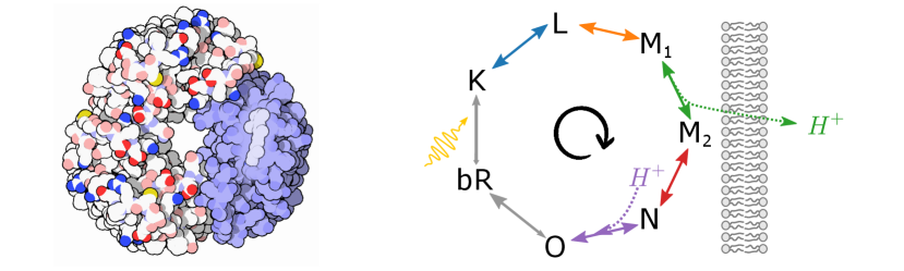
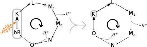
We illustrate our results on bacteriorhodopsin (Fig. 1), a proton-pumping membrane protein. Bacteriorhodopsin is a photosynthetic system found in Archaea, with close relatives in bacteria [20, 21]. It is also used in many artificial light-harvesting systems [7, 9, 8, 11]. Using published thermodynamic and kinetic data, we develop a thermodynamically consistent stochastic model of bacteriorhodopsin. We demonstrate that, under normal operating conditions, the bacteriorhodopsin system is remarkably efficient.
Our main result is formulated as a convex optimization problem which must be solved numerically in the general case. In the second part of this paper, we derive closed-form solutions of this problem for three physically meaningful regimes: the weakly-driven linear response regime, the irreversible deterministic regime, and the intermediate near-deterministic regime. These solutions illustrate how optimal harvesting reflects the “alignment” between free energy input and relaxation dynamics. We illustrate these closed-form solutions on two unicyclic systems, which may be interpreted as idealized models of two types of nonequilibrium harvesting devices.
We finish our paper with a brief Discussion. There we relate our approach to previous work, including maximization of power output in steady-state engines and flux balance analysis. We also propose directions for future research.
II Setup
We consider a system with mesostates described by the distribution . The distribution evolves according to the master equation , where is the transition rate (). Usually represents a probability distribution of a stochastic system with Markovian dynamics [22, 23]. However, under an appropriate choice of units, it may also represent chemical concentrations in a deterministic chemical reaction network with pseudo-first-order reactions, such as an enzymatic cycle [24, 25].
The system is coupled to a heat bath at inverse temperature , an internal free energy reservoir, and a nonequilibrium environment that serves as an external source of free energy. For example, in a metabolic network, one may consider an internal reservoir of ATP and an external source of glucose. The system has nonequilibrium free energy
| (1) |
where is the Shannon entropy and is the internal free energy of mesostate [26].
As mentioned in the Introduction, we suppose that the dynamics of the system can be separated into baseline and control processes. We make one important assumption in our analysis: the control processes are only coupled to the heat bath and internal free energy reservoir, but not directly to the external source of free energy. This means that control can only increase harvesting by interacting with the baseline, rather than directly increasing the inflow of free energy from the external source. For example, in a metabolic network, control processes cannot directly increase the import of glucose, but they can affect the rate at which glucose is converted into ATP by optimizing intermediate reactions and mechanisms. Control processes may be driven by the internal reservoir (e.g., coupled to ATP hydrolysis) or undriven (e.g., enzymes).
To formalize the baseline/control distinction, we write the rate matrix as , where and represent the transition rate of due to baseline and control. Given distribution , the increase of system free energy due to baseline processes is
| (2) |
The increase due to control processes is defined analogously but using rate matrix ,
| (3) |
The harvesting rate is the rate at which free energy flows to the internal reservoir. The harvesting rate due to baseline processes is
| (4) |
where is the free energy increase in the internal reservoir due to a single baseline transition and is the rate of free energy flow to the internal reservoir due to internal transitions within (assuming is a coarse-grained mesostate). Similarly, the harvesting rate due to control processes is
| (5) |
where is the free energy increase in the internal reservoir due to control transition . For simplicity, we assume that control cannot exchange free energy with the internal reservoir due to internal transitions within . Negative values of indicate driving done on the system by the internal reservoir.
For a concrete example of how are defined for a real biomolecular system, see the bacteriorhodopsin example below and SM-II [27].
As standard in stochastic thermodynamics, we assume that control processes obey local detailed balance (LDB) [16, 28],
| (6) |
Eq. (6) guarantees that the irreversibility of each control transition is determined by the amount of free energy dissipated by that transition [29]. Observe that the right side accounts for free energy changes of the system () and the internal reservoir (), but not the external source. This formalizes the assumption that control processes do not exchange free energy with the external source.
We do not require that the baseline rate matrix obeys LDB, although it will often do so for reasons of thermodynamic consistency.
III Maximum harvesting rate
Suppose that the combined rate matrix has the steady-state distribution , which satisfies . The total steady-state harvesting rate due to baseline and control is
| (7) |
We seek to maximize this harvesting rate by varying the parameters of the control processes while holding the baseline parameters () fixed. Finding this maximum would allow us to determine fundamental bounds on harvesting and to evaluate the efficiency of existing harvesting systems.
However, is not a concave function of the parameters , therefore maximization of (7) is not a convex optimization problem and is not generally intractable. In the following, we reformulate this maximization as a convex optimization with a physically interpretable objective. This allows us to solve the optimization numerically and, at least for some special cases, also in closed form.
To begin, we rewrite (7) as
| (8) |
where we introduced the Schnackenberg formula for the entropy production rate (EPR) [22],
| (9) |
where is the one-way probability flux due to control transition .
Eq. (8) has an intuitive physical interpretation: the total steady-state harvesting rate is the rate of free energy increase in the system and internal reservoir due to baseline, minus the rate of dissipation (EPR) due to the control fluxes. The derivation of this result proceeds in two steps (see SM-I.1 [27] for details). The first step is to show that , which follows by combining (9) with (3) and (6). This states that the EPR due to control is proportional to the free energy loss in the system and internal reservoir due to control. The second step is to show that , which follows because the left side is the overall derivative of the nonequilibrium free energy , as defined in (1), therefore it must vanish in steady state. The result (8) then follows by combining with (7) and rearranging.
Importantly, when expressed in the form (8), the harvesting rate is a concave function of the steady-state distribution and the control fluxes (see SM-I.2 [27]). To find the maximum harvesting rate, we optimize (8) with respect to and . Note that varying and is equivalent to varying the control rate matrix via and control driving via (6). However, when performing this optimization, we must also ensure that is the steady-state distribution induced by the fluxes . This condition can be expressed as a linear constraint on and via . Here is treated as a vector in and is the incidence matrix with entries , which guarantees .
Combining, we arrive at the bound , where
| (10) |
In this expression, is the feasible set of distributions and control fluxes . At a minimum, ensures the validity of the distribution and the fluxes via the linear constraints , , and . We write instead of because the set of allowed fluxes is potentially unbounded. Eq. (10) implies a tradeoff between the total gain of free energy in the system and internal reservoir due to baseline (which depends only on ) and the dissipation due to control fluxes (which depends only on ).
Importantly, the feasible set can include additional convex constraints, which may introduce topological, kinetic, thermodynamic, etc. restrictions on the control processes. Topological constraints restrict which transitions can be controlled; e.g., ensures that control does not use transition ). Kinetic constraints restrict timescales of control processes, as might reflect underlying physical processes like diffusion; e.g., an upper bound on control transition rate can be enforced via . Thermodynamic constraints bound the affinity [22] of control transitions; e.g., ensures that . The above examples all involve linear constraints. An example of a nonlinear, but still convex, constraint is an upper bound on the EPR incurred by control, .
Eq. (10) is our first main result. Importantly, is defined purely in terms of the thermodynamic and kinetic properties of the baseline process, along with desired constraints encoded in . Thus, is the maximum steady-state harvesting rate that can be achieved by any allowed control processes, given a fixed baseline. In addition, Eq. (10) involves the maximization of a concave objective given convex constraints. This is equivalent to the minimization of a convex objective, thus Eq. (10) is a convex optimization problem that can be efficiently solved using standard numerical techniques [30]. The optimization also identifies an optimal steady-state distribution and control fluxes that achieve the maximum harvesting rate (or come arbitrarily close to achieving it). These fix the optimal control rate matrix via . Thus, our optimization specifies an upper bound on harvesting as well as the optimal control strategy that achieves this bound.
There is an important special case in which our optimization problem is simplified. Suppose that does not enforce additional constraints on and (more generally, we permit topological constraints if the graph of allowed transitions is connected and contains all states). Then, the objective is maximized in limit of fast control, and . We can then write (10) as an optimization over steady-state distributions:
| (11) |
The optimal is unique as long as the baseline rate matrix is irreducible. The optimal control rate matrix is very fast () and obeys detailed balance for , . For details, see SM-I.3 and SM-I.4 [27].
IV Bacteriorhodopsin
We illustrate our results using bacteriorhodopsin, a light-driven proton pump from Archaea [18].
We define a thermodynamically consistent model of the bacteriorhodopsin cycle using published thermodynamic [31] and kinetic [32] data (see SM-II [27]). The system operates in a cyclical manner, absorbing a photon and pumping a proton during each turn of the cycle (Fig. 1, right). Specifically, the transition pumps a proton out of the cell. This stores free energy in the internal reservoir (the membrane electrochemical potential),
| (12) |
where is the elementary charge constant, is the membrane electrical potential, and is the membrane pH difference. The other transitions in the cycle do not affect the free energy of the internal reservoir ( and ).
During the transition , the system leaves the ground state by absorbing a photon at 580nm, thereby harvesting free energy from the external source and dissipating some heat to the environment at K. This transition is much faster (picoseconds) than the other transitions in the photocycle (micro- to milliseconds). As commonly done in photochemistry [33], we coarse-grain transitions and into a single effective transition .
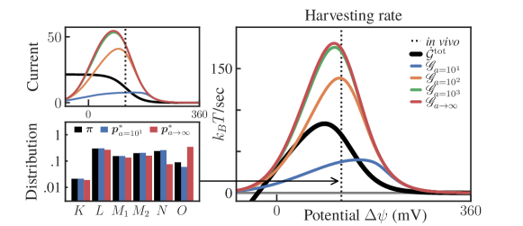
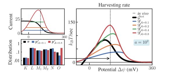
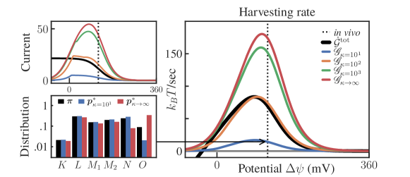
To explore the performance of bacteriorhodopsin under different conditions, we vary the membrane electrical potential between and mV, while using a realistic fixed [34]. We show the actual harvesting rate ( in units of sec) at different potentials as a black line in Fig. 2 (a). At a plausible in vivo mV [34], the model exhibits a steady-state current of 11.5 protons/sec, each proton carrying 6.1 of free energy, corresponding to /sec. The largest output is achieved near the in vivo potential: at lower potentials, the cycle current saturates while the free energy per proton drops, and at higher potentials the pump stalls.
Next, we quantify the maximum harvesting rate that can be achieved by optimizing the parameters of individual transitions. This analysis is relevant for understanding limits on increasing bacteriorhodopsin output, whether via natural selection or biosynthetic methods [35, 36, 37, 38]. Interestingly, such transition-level optimization may be feasible in bacteriorhodopsin, as the properties of several transitions are known to be individually controlled by particular amino acid residues in the bacteriorhodopsin protein [35, 39, 40, 41].
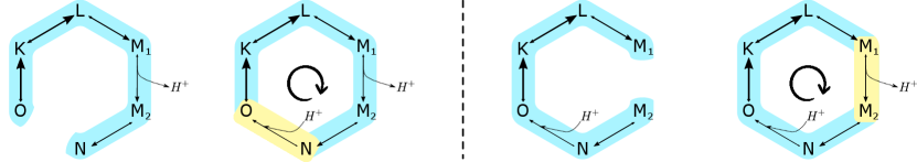
For each reversible transition in the cycle, for instance , we define the baseline as the rest of the cycle without that transition. We then optimize control under the topological constraint that only the relevant transition (e.g., ) is allowed. The analysis is repeated for all transitions, except for the (coarse-grained) photon-absorbing transition , which is in accordance with our assumption that control cannot directly exchange free energy directly with the external source.
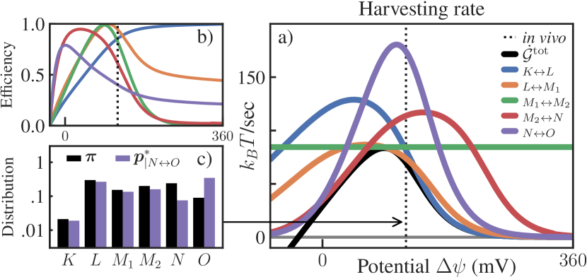
Fig. 2 (a) shows , the maximum achievable by optimizing each reversible transition. In Fig. 2 (b), we also show the efficiency for each transition, that is the ratio of the actual and maximum harvesting rate.
Several transitions, such as ,,, are remarkably efficient () near in vivo membrane potentials. The reprotonation step is the least efficient () and also has the slowest kinetics of the 5 transitions studied in Fig. 2. This suggests that is a bottleneck whose optimization can have a big impact on the harvesting rate, while optimization of other non-bottleneck transitions has a more limited effect.
Observe that for does not depend on . This is because is a function of baseline properties, which do not depend on the membrane potential when is treated as control. Conversely, as control transition can be optimized by varying the membrane potential and/or scaling up the forward/backward rates. Our results show that this transition is very close to optimal at in vivo membrane potentials and kinetic timescales.
Optimal distributions are also obtained, with a typical one shown in Fig. 2 (c). We find a consistent shift toward state , which accelerates the reset of the cycle and increases the flux across the photon-absorbing transition .
In SM-II [27], we illustrate how the efficiency of bacteriorhodopsin transitions can be evaluated under other types of constraints, including constraints on thermodynamic affinity, dynamical activity, and kinetics.
As a final analysis, instead of optimizing individual existing transitions in the bacteriorhodopsin cycle, we ask to what extent the harvesting rate can be increased by any additional control processes. For example, this could involve an additional enzyme that shifts the cycle’s steady state by permitting a new transition between distant states (e.g. ), possibly yielding an increase of the proton pumping rate.
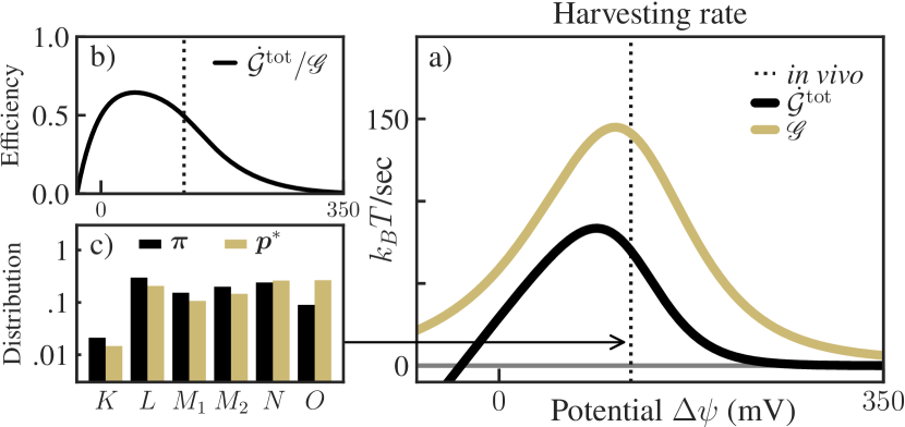
In this case, we treat the entire bacteriorhodopsin system as the baseline, and we do not introduce any additional constraints on the steady-state distribution or the control fluxes. Then, as shown in Sec. SM-I.4 [27], the objective in (10) is achieved in the limit of fast control, and the maximum harvesting rate can be found by solving the simplified optimization problem (11).
For this setup, Fig. 3 (a) shows the baseline (actual) harvesting rate and the maximum harvesting rate at varying . Interestingly, both peak at around the in vivo values of the membrane potential. In Fig. 3 (b), we show that the actual bacteriorhodopsin cycle harvests approximately 50% of the fundamental bound given by (at in vivo values of ). This suggests that bacteriorhodopsin is remarkably close to optimal, relative to improvements that could be achieved by introducing any additional control processes.
We also show the actual steady-state distribution and the optimal distribution in Fig. 3 (c). The optimal distribution increases the probability of state , similar to the optimal distribution found by optimizing the transition, shown in Fig. 2 (c). However, unlike Fig. 2 (c), where most of the extra probability is taken from state , in Fig. 3 (c) the probability is drawn more uniformly from other states in the cycle, indicating the presence of distributed control.
V Limiting regimes
Our results are stated via an optimization problem that generally does not have a closed-form solution. In our second set of results, we identify closed-form expressions in three physically meaningful regimes. For simplicity, here we focus on the simplified objective (11). See SM-III [27] for detailed derivations, including analysis of the conditions under which each of these three approximation are be valid.
For convenience, we first rewrite (11) as
| (13) |
where is the increase of the Shannon entropy of under and for convenience we defined . The objective (13) contains a nonlinear term quantifying the decrease of information-theoretic entropy and a linear term quantifying the flow of thermodynamic free energy.
Next, we consider three regimes.
Linear response (LR) applies when the optimal distribution is close to the steady-state distribution of the baseline rate matrix . Suppose that is irreducible and has a unique steady state with full support. We introduce the “additive reversibilization” of ,
| (14) |
The rate matrix obeys detailed balance (DB) for the steady-state distribution and has the same dynamical activity [42] on all edges as . may be considered as a DB version of , and it is equal to when the latter obeys DB [43, 44]. Let indicate the -th right eigenvector of normalized as , and the corresponding real-valued eigenvalue (). The LR solution for the maximum harvesting rate and the optimal distribution is
| (15) |
where quantifies the harvesting “amplitude” for mode .
Eq. (15) has a simple interpretation. In addition to the baseline harvesting rate , contains contributions from the relaxation modes of , with each mode weighed by its squared amplitude and relaxation timescale . All else being equal, is large when slow modes have large harvesting amplitudes. The optimal shifts the baseline steady state toward mode in proportion to that mode’s harvesting amplitude and relaxation timescale, thereby optimally balancing the tradeoff between harvesting and dissipation.
The Deterministic (D) regime applies when the nonlinear information-theoretic term in (13) is much smaller than the linear thermodynamic term. We can then ignore the former, turning (13) into a simple linear optimization. This gives the approximate solution
| (16) |
where is the optimal mesostate. This solution concentrates probability on a single mesostate, effectively ignoring the cost of maintaining this low-entropy distribution.
The Near-Deterministic (ND) regime lies between Linear Response and Deterministic ones. By perturbing around , we can decouple the values of in the objective function (11). The maximal harvesting rate and optimal distribution in this regime are then given by
| (17) |
The ND solution also has a simple interpretation. It perturbs the Deterministic solution by shifting probability towards states with high transition rates away from the optimal state (large ) and small decreases in harvesting (). This balances the benefit of harvesting against the cost of pumping probability against .
VI Example: unicyclic systems
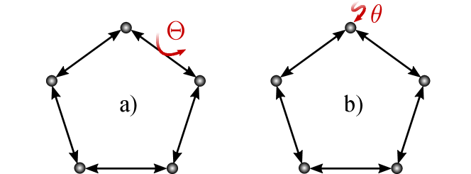
We illustrate our closed-form solutions using two simple models, both based on a unicyclic system with states. The baseline dynamics involve diffusion across a 1-dimensional ring, with left and right jump rates set to 1. The baseline steady state is a uniform distribution, , with no cyclic current. We assume a uniform free energy function, for all .
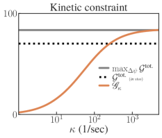
We consider two different scenarios. In the first scenario, shown schematically in Fig. 4 (a), of free energy is harvested each time the system carries out the transition , so
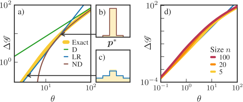
and otherwise. This scenario may be interpreted as an idealized model of a biomolecular harvesting cycle, such as a transporter. In the second scenario, shown schematically in Fig. 4 (b), free energy is harvested at a rate of per unit time when the system is located in one particular mesostate , so
| (18) |
and otherwise. This scenario may be interpreted as an idealized model of error correction or self-assembly, where free energy can only be harvested when the system is in some particular functional mesostate.
For both scenarios, we evaluate the maximum harvesting rate and the optimal distributions achievable by adding any possible control to the system, without constraints. We report exact values found by numerical optimization of Eq. (13), as well as the LR, ND, and D approximations described above. To calculate the LR values, we exploit the fact that the baseline unicyclic rate matrix is a circulant matrix with a simple eigendecomposition [45]. Full details of the derivations for the two scenarios are provided in SM-IV [27] and SM-IV.3 [27], respectively.
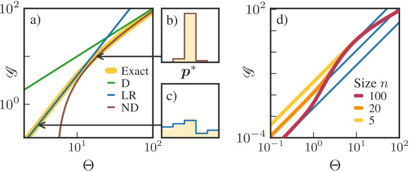
We first report results for the first scenario from Fig. 4 (a), where free energy is harvested during the transition . Observe that baseline harvesting rate vanishes, , since harvesting free energy requires a cyclic current. In Fig. 5 (a), we plot the maximum harvesting rate and its approximations as a function of the supplied free energy . For small , LR applies and the maximum harvesting rate is
| (19) |
The optimal distribution in the LR regime, shown in Fig. 5 (c), builds up in equal increments starting from until the optimal state , after which it drops sharply. For large , the D regime is relevant and the optimal distribution concentrates on the optimal state , so
| (20) |
At intermediate , the ND regime applies, which gives
| (21) |
The optimal distribution in the ND regime, shown in Fig. 5 (b), allocates , and the rest to the optimal state .
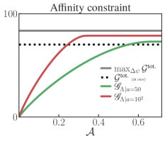
Next, we consider the second scenario from Fig. 4 (b), where free energy is harvested when the system is in the optimal mesostate . Observe that the uniform baseline steady state assigns probability to the optimal state, thus in this scenario the baseline harvesting rate is . To facilitate comparison with the first scenario, we focus on the increase of the maximum harvesting rate relative to baseline,
| (22) |
In Fig. 6 (a), we show and its approximations as a function of the free energy supply rate . For small , LR applies and the maximum harvesting rate is
| (23) |
The optimal distribution in the LR regime, shown in Fig. 6 (c), is symmetric about the optimal state . For large , the D regime is relevant and the optimal distribution concentrates on the optimal state , so
| (24) |
At intermediate , the ND regime applies, giving
| (25) |
The optimal distribution in the ND regime, shown in Fig. 6 (b), allocates and the rest to .
There are some similarities among the two harvesting scenarios. For both scenarios, in the LR regime, the increase of the harvesting rate scales quadratically in the supplied free energy ( or ) and linearly in inverse temperature . This scaling reflects the fact that the optimal strategy has to balance harvesting ( or contributions) with the thermodynamic cost of maintaining a low entropy ( contributions). In the ND and D regimes, scales linearly in the supplied free energy and loses its linear dependence on . Thus, outside of LR, the thermodynamic cost of maintaining a low entropy distribution has a minor effect on the optimal strategy.
There are also important differences between the two scenarios. For the first scenario, the optimal strategy maintains an asymmetric , thereby generating a net flux across the transition . In the LR regime, the cost of maintaining this asymmetric distribution grows with the system size , therefore the maximum harvesting rate in Eq. (19) scales as . This is shown in Fig. 5 (d), where we plot and its LR approximation at various and . For the second scenario, the optimal strategy maintains a peaked but symmetric . Remarkably, the cost of maintaining this distribution does not depend on system size . This is shown in Fig. 6 (d), where we plot at various and .
VII Discussion
In this paper, we consider the problem of optimizing free energy harvesting in a nonequilibrium steady-state system. We demonstrate that this problem can be formulated as a constrained convex optimization problem, and we use this formulation to study optimal harvesting and efficiency in the bacteriorhodopsin proton pump. We also solve the convex optimization problem in closed-form for three limiting regimes, as illustrated on two unicyclic models discussed above.
A key step in our analysis is to separate the dynamics of the system into separate contributions from fixed baseline processes and optimizable control processes. We note that, in stochastic thermodynamics, the baseline/control separation has been previously used to study autonomous Maxwellian demons [46, 47], counterdiabatic driving [48], and the cost of maintaining a nonequilibrium steady state [49, 50].
We derive a simplified bound on the maximum harvesting rate in (13), which is achieved in the limit of fast dissipation-less control. Interestingly, this expression involves a tradeoff between two terms, one information-theoretic and one thermodynamic. At first glance, this resembles information/free-energy tradeoffs characteristic of Maxwellian demons and other “information engines” [51, 52, 53, 54, 55, 56, 57, 58]. However, there are important differences. In a typical information engine, there is no external source of driving and information serves as fuel, which can be converted into of thermodynamic free energy per bit. In our case, there is an external source of free energy that in some cases can be harvested more effectively by reducing the system’s statistical entropy, e.g. by concentrating it on favorable states. Here, a bit of information can increase the harvesting rate by a very large amount (much larger than ), and information acts more like a catalyst than a fuel [59, 60]. Loosely speaking, this is similar to how information encoded in the sequence of a metabolic enzyme is not itself fuel, but rather allows metabolism to harvest a large amount of fuel from elsewhere.
We finish by mentioning some connections to previous work and future directions. First, our approach may be related to prior work on optimizing power output and free energy transduction in steady-state molecular machines [61, 62, 63, 64, 65, 29, 66]. Here we consider the general problem of optimizing a set of control processes, given a fixed baseline and possible additional constraints on kinetics, topology, and thermodynamics. Previous work does not make the baseline/control distinction; instead, it is mostly concerned with the problem of optimizing system performance with respect to a small set of specific parameters or observables of interest, such as the location of free energy barriers [66, 62, 63, 65], efficiency [66], and the size of fluctuations [61, 64].
There is also an interesting relation between our work and flux balance analysis (FBA) [67, 68, 69]. The goal of FBA is to identify deterministic fluxes in biological metabolic systems that optimize biomass production, or other similar metrics of performance. This can be formulated as a linear program, which may include linear constraints that enforce thermodynamically favored reaction directions [69] (interestingly, in Ref. [70], the authors propose a version of FBA that also accounts for the entropy production rate). Our setting and optimization are different from FBA and its variants. We seek to optimize free energy harvesting at the stochastic level, and our objective involves nonlinear information-theoretic contributions to free energy. In addition, our optimization involves both the steady-state distribution and fluxes , which allows us to optimize harvesting due to to internal transitions within coarse-grained mesostates, as in Fig. 4 (b). Nonetheless, investigating the relationship between our approach and FBA is an interesting direction for future work.
Another interesting direction for future work is to consider stochastic fluctuations of free energy harvesting. In particular, the thermodynamic uncertainty relation may be used to study tradeoffs between the entropy production rate, the average harvesting rate (the quantity considered here), and the fluctuations in the amount of harvested free energy [71, 64]. For biomolecular systems, large fluctuations in harvesting can lead to starvation, suggesting that minimizing fluctuations may be of significant biological importance.
Finally, an interesting direction for future work is to consider free energy harvesting in a system embedded in a fluctuating environment. For example, one may imagine a harvesting system in an environment with fluctuating sugar sources, or with a fluctuating amount of available light. In this setting, it is natural to optimize the harvesting rate under the topological constraint that control fluxes cannot directly change the state of the environment, for instance using bipartite models of Markovian dynamics [72]. It would be interesting to investigate how, under the optimal harvesting strategy, the information flow from the environment to the system varies with the abundance of free energy and complexity of the environment.
Acknowledgements.
We thank members of the Complex Systems Lab, B. Corominas-Murtra, L. Seoane, D. Wolpert, and D. Sowinski for useful discussions. A.K. also thanks Sosuke Ito for support and encouragement. This project has received funding from the European Union’s Horizon 2020 research and innovation programme under the Marie Skłodowska-Curie Grant Agreement No. 101068029. J.P. was supported by the María de Maeztú fellowship MDM-2014-0370-17-2 and Grant No. 62417 from the John Templeton Foundation. The opinions expressed in this publication are those of the authors and do not necessarily reflect the views of the John Templeton Foundation.References
- [1] T. L. Hill, Free energy transduction in biology: the steady-state kinetic and thermodynamic formalism. New York: Academic Press, 1977.
- [2] H. Morowitz, Foundations of bioenergetics. Elsevier, 2012.
- [3] A. J. Lotka, “Contribution to the energetics of evolution,” Proceedings of the National Academy of Sciences, vol. 8, no. 6, pp. 147–151, 1922.
- [4] J. H. Brown, P. A. Marquet, and M. L. Taper, “Evolution of body size: consequences of an energetic definition of fitness,” The American Naturalist, vol. 142, no. 4, pp. 573–584, 1993.
- [5] W. B. Watt, “Bioenergetics and evolutionary genetics: opportunities for new synthesis,” The American Naturalist, vol. 125, no. 1, pp. 118–143, 1985.
- [6] O. P. Judson, “The energy expansions of evolution,” Nature ecology & evolution, vol. 1, no. 6, p. 0138, 2017.
- [7] H.-J. Choi and C. D. Montemagno, “Artificial organelle: Atp synthesis from cellular mimetic polymersomes,” Nano letters, vol. 5, no. 12, pp. 2538–2542, 2005.
- [8] K. Y. Lee, S.-J. Park, K. A. Lee, S.-H. Kim, H. Kim, Y. Meroz, L. Mahadevan, K.-H. Jung, T. K. Ahn, K. K. Parker, et al., “Photosynthetic artificial organelles sustain and control atp-dependent reactions in a protocellular system,” Nature biotechnology, vol. 36, no. 6, pp. 530–535, 2018.
- [9] S. Berhanu, T. Ueda, and Y. Kuruma, “Artificial photosynthetic cell producing energy for protein synthesis,” Nature communications, vol. 10, no. 1, p. 1325, 2019.
- [10] K. Villa and M. Pumera, “Fuel-free light-driven micro/nanomachines: Artificial active matter mimicking nature,” Chemical Society Reviews, vol. 48, no. 19, pp. 4966–4978, 2019.
- [11] C. Kleineberg, C. Wölfer, A. Abbasnia, D. Pischel, C. Bednarz, I. Ivanov, T. Heitkamp, M. Börsch, K. Sundmacher, and T. Vidaković-Koch, “Light-driven atp regeneration in diblock/grafted hybrid vesicles,” ChemBioChem, vol. 21, no. 15, pp. 2149–2160, 2020.
- [12] T. E. Miller, T. Beneyton, T. Schwander, C. Diehl, M. Girault, R. McLean, T. Chotel, P. Claus, N. S. Cortina, J.-C. Baret, et al., “Light-powered co2 fixation in a chloroplast mimic with natural and synthetic parts,” Science, vol. 368, no. 6491, pp. 649–654, 2020.
- [13] C. Guindani, L. C. da Silva, S. Cao, T. Ivanov, and K. Landfester, “Synthetic cells: From simple bio-inspired modules to sophisticated integrated systems,” Angewandte Chemie, vol. 134, no. 16, p. e202110855, 2022.
- [14] P. Albanese, F. Mavelli, and E. Altamura, “Light energy transduction in liposome-based artificial cells,” Frontiers in Bioengineering and Biotechnology, vol. 11, p. 1161730, 2023.
- [15] N. S. Chandel, “Glycolysis,” Cold Spring Harbor Perspectives in Biology, vol. 13, no. 5, p. a040535, 2021.
- [16] U. Seifert, “Stochastic thermodynamics, fluctuation theorems and molecular machines,” Reports on progress in physics, vol. 75, no. 12, p. 126001, 2012.
- [17] J. C. Doyle, B. A. Francis, and A. R. Tannenbaum, Feedback control theory. Courier Corporation, 2013.
- [18] J. K. Lanyi, “Bacteriorhodopsin,” Annu. Rev. Physiol., vol. 66, pp. 665–688, 2004.
- [19] D. Goodsell, “Bacteriorhodopsin,” The RSCB PDB Molecule of the Month, vol. 3, 2002. doi:10.2210/rcsb_pdb/mom_2002_3.
- [20] O. Béja, L. Aravind, E. V. Koonin, M. T. Suzuki, A. Hadd, L. P. Nguyen, S. B. Jovanovich, C. M. Gates, R. A. Feldman, J. L. Spudich, et al., “Bacterial rhodopsin: evidence for a new type of phototrophy in the sea,” Science, vol. 289, no. 5486, pp. 1902–1906, 2000.
- [21] L. Gómez-Consarnau, J. A. Raven, N. M. Levine, L. S. Cutter, D. Wang, B. Seegers, J. Arístegui, J. A. Fuhrman, J. M. Gasol, and S. A. Sañudo-Wilhelmy, “Microbial rhodopsins are major contributors to the solar energy captured in the sea,” Science advances, vol. 5, no. 8, p. eaaw8855, 2019.
- [22] J. Schnakenberg, “Network theory of microscopic and macroscopic behavior of master equation systems,” Reviews of Modern physics, vol. 48, no. 4, p. 571, 1976.
- [23] M. Esposito and C. Van den Broeck, “Three faces of the second law. i. master equation formulation,” Physical Review E, vol. 82, no. 1, p. 011143, 2010.
- [24] A. Wachtel, R. Rao, and M. Esposito, “Thermodynamically consistent coarse graining of biocatalysts beyond michaelis–menten,” New Journal of Physics, vol. 20, no. 4, p. 042002, 2018.
- [25] A. Cornish-Bowden, Fundamentals of enzyme kinetics. John Wiley & Sons, 2013.
- [26] J. M. Horowitz, T. Sagawa, and J. M. Parrondo, “Imitating chemical motors with optimal information motors,” Physical review letters, vol. 111, no. 1, p. 010602, 2013.
- [27] See Supplemental Material at [URL will be inserted by publisher] for a derivation of our main results, a full description of the bacteriorhodopsin model and the details for the analyses of limiting regimes and unicyclic examples.
- [28] C. Maes, “Local detailed balance,” SciPost Physics Lecture Notes, p. 032, 2021.
- [29] A. I. Brown and D. A. Sivak, “Theory of nonequilibrium free energy transduction by molecular machines,” Chemical Reviews, vol. 120, pp. 434–459, Jan. 2020.
- [30] S. P. Boyd and L. Vandenberghe, Convex optimization. Cambridge university press, 2004.
- [31] G. Varo and J. K. Lanyi, “Thermodynamics and energy coupling in the bacteriorhodopsin photocycle,” Biochemistry, vol. 30, no. 20, pp. 5016–5022, 1991.
- [32] V. A. Lórenz-Fonfría and H. Kandori, “Spectroscopic and kinetic evidence on how bacteriorhodopsin accomplishes vectorial proton transport under functional conditions,” Journal of the American Chemical Society, vol. 131, pp. 5891–5901, Apr. 2009.
- [33] E. Penocchio, R. Rao, and M. Esposito, “Nonequilibrium thermodynamics of light-induced reactions,” The Journal of Chemical Physics, vol. 155, no. 11, 2021.
- [34] J. K. Lanyi, “Light energy conversion in Halobacterium halobium,” Microbiological Reviews, vol. 42, no. 4, pp. 682–706, 1978.
- [35] A. Miller and D. Oesterhelt, “Kinetic optimization of bacteriorhodopsin by aspartic acid 96 as an internal proton donor,” Biochimica et Biophysica Acta (BBA)-Bioenergetics, vol. 1020, no. 1, pp. 57–64, 1990.
- [36] A. Seitz and N. Hampp, “Kinetic optimization of bacteriorhodopsin films for holographic interferometry,” The Journal of Physical Chemistry B, vol. 104, no. 30, pp. 7183–7192, 2000.
- [37] K. J. Wise, N. B. Gillespie, J. A. Stuart, M. P. Krebs, and R. R. Birge, “Optimization of bacteriorhodopsin for bioelectronic devices,” Trends in biotechnology, vol. 20, no. 9, pp. 387–394, 2002.
- [38] J. R. Hillebrecht, K. J. Wise, J. F. Koscielecki, and R. R. Birge, “Directed evolution of bacteriorhodopsin for device applications,” in Methods in enzymology, vol. 388, pp. 333–347, Elsevier, 2004.
- [39] J. Tittor, M. Wahl, U. Schweiger, and D. Oesterhelt, “Specific acceleration of de-and reprotonation steps by azide in mutated bacteriorhodopsins,” Biochimica et Biophysica Acta (BBA)-Bioenergetics, vol. 1187, no. 2, pp. 191–197, 1994.
- [40] S. P. Balashov, M. Lu, E. S. Imasheva, R. Govindjee, T. G. Ebrey, B. Othersen, Y. Chen, R. K. Crouch, and D. R. Menick, “The proton release group of bacteriorhodopsin controls the rate of the final step of its photocycle at low ph,” Biochemistry, vol. 38, no. 7, pp. 2026–2039, 1999.
- [41] Q. Li, S. Bressler, D. Ovrutsky, M. Ottolenghi, N. Friedman, and M. Sheves, “On the protein residues that control the yield and kinetics of o630 in the photocycle of bacteriorhodopsin,” Biophysical Journal, vol. 78, no. 1, pp. 354–362, 2000.
- [42] The dynamical activity refers to the overall rate of back-and-forth jumps across a transitions, .
- [43] A. Kolchinsky, N. Ohga, and S. Ito, “Thermodynamic bound on spectral perturbations, with applications to oscillations and relaxation dynamics,” Physical Review Research, vol. 6, no. 1, p. 013082, 2024.
- [44] J. A. Fill, “Eigenvalue bounds on convergence to stationarity for nonreversible Markov chains, with an application to the exclusion process,” The Annals of Applied Probability, vol. 1, no. 1, pp. 62–87, 1991.
- [45] R. M. Gray et al., “Toeplitz and circulant matrices: A review,” Foundations and Trends® in Communications and Information Theory, vol. 2, no. 3, pp. 155–239, 2006.
- [46] N. Shiraishi, S. Ito, K. Kawaguchi, and T. Sagawa, “Role of measurement-feedback separation in autonomous maxwell’s demons,” New Journal of Physics, vol. 17, no. 4, p. 045012, 2015.
- [47] N. Shiraishi, T. Matsumoto, and T. Sagawa, “Measurement-feedback formalism meets information reservoirs,” New Journal of Physics, vol. 18, no. 1, p. 013044, 2016.
- [48] K. Takahashi, K. Fujii, Y. Hino, and H. Hayakawa, “Nonadiabatic control of geometric pumping,” Physical Review Letters, vol. 124, no. 15, p. 150602, 2020.
- [49] J. M. Horowitz and J. L. England, “Information-theoretic bound on the entropy production to maintain a classical nonequilibrium distribution using ancillary control,” Entropy, vol. 19, no. 7, p. 333, 2017.
- [50] J. M. Horowitz, K. Zhou, and J. L. England, “Minimum energetic cost to maintain a target nonequilibrium state,” Physical Review E, vol. 95, no. 4, p. 042102, 2017.
- [51] J. M. Parrondo, J. M. Horowitz, and T. Sagawa, “Thermodynamics of information,” Nature Physics, vol. 11, no. 2, pp. 131–139, 2015.
- [52] T. Sagawa and M. Ueda, “Minimal energy cost for thermodynamic information processing: measurement and information erasure,” Physical review letters, vol. 102, no. 25, p. 250602, 2009.
- [53] D. Abreu and U. Seifert, “Thermodynamics of genuine nonequilibrium states under feedback control,” Physical review letters, vol. 108, no. 3, p. 030601, 2012.
- [54] F. J. Cao and M. Feito, “Thermodynamics of feedback controlled systems,” Physical Review E, vol. 79, no. 4, p. 041118, 2009.
- [55] S. Ito and T. Sagawa, “Information thermodynamics on causal networks,” Physical review letters, vol. 111, no. 18, p. 180603, 2013.
- [56] D. Hartich, A. C. Barato, and U. Seifert, “Stochastic thermodynamics of bipartite systems: transfer entropy inequalities and a Maxwell’s demon interpretation,” Journal of Statistical Mechanics: Theory and Experiment, vol. 2014, no. 2, p. P02016, 2014.
- [57] A. C. Barato, D. Hartich, and U. Seifert, “Efficiency of cellular information processing,” New Journal of Physics, vol. 16, no. 10, p. 103024, 2014.
- [58] P. Sartori, L. Granger, C. F. Lee, and J. M. Horowitz, “Thermodynamic costs of information processing in sensory adaptation,” PLoS Comput Biol, vol. 10, no. 12, p. e1003974, 2014.
- [59] J. Barham, “A dynamical model of the meaning of information,” Biosystems, vol. 38, no. 2-3, pp. 235–241, 1996.
- [60] A. Kolchinsky and D. H. Wolpert, “Semantic information, autonomous agency and non-equilibrium statistical physics,” Interface Focus, vol. 8, p. 20180041, Dec. 2018.
- [61] P. Pietzonka, A. C. Barato, and U. Seifert, “Universal bound on the efficiency of molecular motors,” Journal of Statistical Mechanics: Theory and Experiment, vol. 2016, p. 124004, Dec. 2016.
- [62] A. I. Brown and D. A. Sivak, “Allocating dissipation across a molecular machine cycle to maximize flux,” Proceedings of the National Academy of Sciences, vol. 114, no. 42, pp. 11057–11062, 2017.
- [63] A. I. Brown and D. A. Sivak, “Allocating and splitting free energy to maximize molecular machine flux,” The Journal of Physical Chemistry B, vol. 122, no. 4, pp. 1387–1393, 2018.
- [64] P. Pietzonka and U. Seifert, “Universal Trade-Off between Power, Efficiency, and Constancy in Steady-State Heat Engines,” Physical Review Letters, vol. 120, p. 190602, May 2018.
- [65] J. A. Wagoner and K. A. Dill, “Mechanisms for achieving high speed and efficiency in biomolecular machines,” Proceedings of the National Academy of Sciences, vol. 116, no. 13, pp. 5902–5907, 2019.
- [66] T. Schmiedl and U. Seifert, “Efficiency of molecular motors at maximum power,” EPL (Europhysics Letters), vol. 83, no. 3, p. 30005, 2008.
- [67] D. A. Beard, S.-d. Liang, and H. Qian, “Energy balance for analysis of complex metabolic networks,” Biophysical journal, vol. 83, no. 1, pp. 79–86, 2002.
- [68] K. J. Kauffman, P. Prakash, and J. S. Edwards, “Advances in flux balance analysis,” Current opinion in biotechnology, vol. 14, no. 5, pp. 491–496, 2003.
- [69] M. Kschischo, “A gentle introduction to the thermodynamics of biochemical stoichiometric networks in steady state,” The European Physical Journal Special Topics, vol. 187, no. 1, pp. 255–274, 2010.
- [70] R. M. Fleming, C. M. Maes, M. A. Saunders, Y. Ye, and B. Ø. Palsson, “A variational principle for computing nonequilibrium fluxes and potentials in genome-scale biochemical networks,” Journal of theoretical biology, vol. 292, pp. 71–77, 2012.
- [71] T. R. Gingrich, J. M. Horowitz, N. Perunov, and J. L. England, “Dissipation bounds all steady-state current fluctuations,” Physical review letters, vol. 116, no. 12, p. 120601, 2016.
- [72] J. M. Horowitz and M. Esposito, “Thermodynamics with continuous information flow,” Physical Review X, vol. 4, no. 3, p. 031015, 2014.
- [73] M. Esposito, “Stochastic thermodynamics under coarse graining,” Physical Review E, vol. 85, no. 4, p. 041125, 2012.
- [74] T. M. Cover and J. A. Thomas, Elements of information theory. John Wiley & Sons, 2006.
- [75] E. Ilker, Ö. Güngör, B. Kuznets-Speck, J. Chiel, S. Deffner, and M. Hinczewski, “Shortcuts in stochastic systems and control of biophysical processes,” Physical Review X, vol. 12, no. 2, p. 021048, 2022.
- [76] A. M. Ferreira and D. Bashford, “Model for proton transport coupled to protein conformational change: application to proton pumping in the bacteriorhodopsin photocycle,” Journal of the American Chemical Society, vol. 128, no. 51, pp. 16778–16790, 2006.
- [77] J. K. Lanyi, “Halorhodopsin: a light-driven chloride ion pump,” Annual review of biophysics and biophysical chemistry, vol. 15, no. 1, pp. 11–28, 1986.
- [78] S. Ahmed and I. R. Booth, “The use of valinomycin, nigericin and trichlorocarbanilide in control of the protonmotive force in escherichia coli cells,” Biochemical Journal, vol. 212, no. 1, pp. 105–112, 1983.
- [79] C. Naslund, “Mathematics stackexchange. question 104967,” 2012. https://math.stackexchange.com/questions/104967/.
- [80] Svyatoslav and C. Leibovici, “Mathematics stackexchange. question 4567421,” 2022. https://math.stackexchange.com/questions/4567421/.
Supplemental Material:
Optimization of nonequilibrium free energy harvesting illustrated on bacteriorhodopsin
Jordi Piñero, Ricard Solé, and Artemy Kolchinsky
I Derivations of main results
I.1 Derivation of (8) from LDB and steady-state assumption
Here we derive (8) in the main text, which reads as
| (S1.1) |
To derive this result,
| (S1.2) |
The first line follows from definitions made in the main text. Since is a rate matrix, for any . This allows us to further rewrite (S1.2) as
| (S1.3) |
In the second line, we plugged in the condition of LDB, as expressed in (6) in the main text:
| (S1.4) |
Using the definition of one-way fluxes due to control given a generic distribution , , and the Schnackenberg expression of EPR , we rewrite (S1.3) as
| (S1.5) |
In the main text, this equality is applied at the steady-state distribution . However, Eq. (S1.5) is valid for all distributions as long as (S1.4) holds.
To complete our derivation of (S1.1), recall that by definition of the steady-state . At the same time, from the definition of in (2), we have
| (S1.6) |
Combining the definition of with (S1.5) and (S1.6) gives Eq. (S1.1),
| (S1.7) |
Finally, note that the entropy production rate is always nonnegative:
| (S1.8) |
where the last inequality follows because the terms and have the same sign. This can be seen as a statement of the Second Law.
Let us briefly comment on the physical meaning of our derivation. First, we note that LDB holds when the control dynamics exhibit a separation of timescales, with fast equilibration within each mesostate and slower transitions between mesostates [73].
Second, recall our assumption that the control processes do not interact directly with the external source of free energy, but only with the internal reservoir and heat bath. This assumption is formalized in the particular form of the LDB condition (S1.4). It means that for the control processes, the combined “system+internal reservoir” may be treated as a single system coupled only to a heat bath at inverse temperature . Hence, the rate of entropy production due to control is simply times the decrease of the combined free energy of the system and internal reservoir, as in (S1.5). Moreover, owing to Second Law, their combined free energy cannot increase under control dynamics [26, 29],
| (S1.9) |
I.2 Concavity of constrained optimization (10)
Consider the objective in (10) in the main text. In Sec. I.3 below, we show that the term is concave in . Here we show that is convex in . This shows that the overall objective is concave in the pair .
Consider any pair of feasible fluxes and and let indicate their convex mixture. To prove convexity, we write
| (S1.10) |
Here we used the log-sum inequality [74, Thm. 2.7.1],
| (S1.11) |
I.3 Properties of the unconstrained optimization (11)
I.3.1 Concavity and existence of maximizer
Consider the objective in (11), as equivalently written in (13):
| (S1.12) |
where is the rate of increase of the Shannon entropy of distribution under the rate matrix . Here we show that is concave, thus (11) involves the maximization of a concave function. This is equivalent to the minimization of a convex function, making it convex optimization problem which can be solved using standard numerical techniques. We also show the existence of a maximizer
Existence of : The feasible set is compact (-dimensional probability simplex) and the objective is continuous, so the maximizer exists by the extreme value theorem. Also, the maximum value is finite (see (S3.86)).
Concavity: Consider any pair of distributions and , and let indicate their convex mixture. We will show that the objective is concave:
| (S1.13) |
Observe that is linear in , thus we can use (S1.12) to rearrange (S1.13) as
| (S1.14) |
To prove (S1.14), we first rewrite the rate of decrease of the Shannon entropy as
| (S1.15) |
Here we first used that for any , then used that the diagonal terms of the sum () vanish. Next, we use (S1.15) to prove (S1.14) as
| (S1.16) | ||||
The second line follows from the log-sum inequality (S1.11).
I.3.2 Strict concavity and uniqueness of maximizer under irreducibility assumption
We can prove further results under the assumption that the baseline rate matrix is irreducible (i.e., there is a path of non-zero transitions connecting any two states) and has a steady-state with full support ( for all ). In graph theoretic terms, this means that the graph of allowed transitions under is strongly connected. Specifically, we prove that our objective is strictly concave, and that the optimizer is unique and has full support.
Strict concavity: The log-sum inequality (S1.11) is strict when [74, Thm. 2.7.1]. In our case, (S1.16) is strict for any pair of states that have and
| (S1.17) |
Such a pair of states must exist, as we now prove by contradiction. Suppose to the contrary that (S1.17) is an equality for all where . Consider a walk on the graph defined by the allowed transitions in — that is, a sequence of states such that . We would then have that , hence also (by multiplication) that . Now, since is irreducible, any state can be reached from any other, implying that for all , hence . Since probabilities are nonnegative and normalized to sum to 1, this can only hold when , contradicting our assumption that in (S1.16).
To summarize, there must be some such that the corresponding term in (S1.16) is a strict inequality, therefore
| (S1.18) |
Uniqueness of maximizer: Suppose that there are two different maximizers, . Then, (S1.18) implies that the convex mixture would achieve a larger value than , leading to a contradiction.
Full support of : Suppose that the maximizer did not have full support, so that some states have 0 probability. Then, there must be some pair such that and and (otherwise the graph of allowed transitions would not be strongly connected). But for this pair, . Plugging into (S1.15) implies that and contradicting the fact that is a maximizer. Hence, must have full support.
I.4 Derivation and achievability of unconstrained optimization (11)
In this section, we derive the unconstrained optimization (11) from the constrained optimization (10).
First, observe that that the maximum in (10) is always less than the maximum in (11):
This follows from nonnegativity of and the fact that (11) has less constraints than (10).
We will show that as long as the feasible set is not too constrained. In addition to the basic normalization and nonnegativity constraints on and , we allow to encode a set of topological constraints like
| (S1.19) |
for , where is a symmetric matrix that determines the topology of the control dynamics ( when the transition is allowed, and otherwise ). We assume that is connected and contains all states. Of course, we may have for all , in which case no topological constraints are imposed. We assume that includes no other constraints.
Given these assumptions, we construct a sequence of control process which satisfy LDB such that:
-
1.
The combined steady state of and control fluxes belong to for all .
-
2.
The combined steady state obeys , where is the optimizer of (11).
-
3.
The steady-state EPR vanishes , therefore the steady-state harvesting rate obeys
Our proof technique is related to the idea sketched out in Ref. [50], which studied the minimal cost of maintaining a nonequilibrium steady state. It is also related to constructions from the literature on counterdiabatic driving [75].
I.4.1 Construction of optimal control
We define a sequence of control processes parameterized by . For each control process, the free energy exchanges with the internal reservoir are set to
| (S1.20) |
The control rate matrix is defined by scaling a given rate matrix
| (S1.21) |
Here is an overall rate constant and is the matrix discussed in (S1.19). The particular choice of the topology encoded in is arbitrary, given our assumption that it is connected and contains all states which guarantees that is irreducible. It can be verified that the rate matrix defined in (S1.21) obeys LDB (6). It also satisfies detailed balance (DB) for the distribution ,
| (S1.22) |
This implies that is the unique steady-state distribution, .
I.4.2 Achievability of the steady state
We show that , the steady-state of the combined rate matrix of , approaches in the limit of fast control (large ). Since and , we have
| (S1.23) |
Rearranging and applying the Moore-Penrose inverse to both sides gives
| (S1.24) |
Since is irreducible by construction, . Plugging into (S1.24), we obtain
| (S1.25) |
which follows from . Taking norms gives
| (S1.26) |
where in the last step we used that the norm of any probability distribution is bounded by 1. This shows that , meaning that the combined steady-state converges to .
I.4.3 EPR vanishes
The steady-state EPR incurred by rate matrix is
| (S1.27) |
Next, we use (S1.25) to write . Using the DB condition for with respect to obtained in (S1.22), we rearrange terms to find:
| (S1.28) |
Plugging into (S1.27) gives
| (S1.29) |
Taking the limit shows that EPR vanishes:
where we used and the DB condition (S1.22) in the logarithmic factor.
II Bacteriorhodopsin model
II.1 Details of model
Here we provide thermodynamic and kinetic details of the bacteriorhodopsin model analyzed in the main text.
The thermodynamic parameters are taken from Ref. [31], which reports in vitro measurements of internal free energies at . Based on Fig. 7 in that paper, we use the following internal free energies for the 6 cycle states:
| (S2.30) |
All values are referenced from the ground state, in other words the zero point refers to the internal free energy of the ground state [31]. However, since we coarse-grain the transitions and into a single transition , we do not include this ground state in our model. See Fig. S7 for an illustration of the coarse-graining.
We use to indicate the free energy transferred to the internal reservoir by the jump from state to state . Only transitions between neighboring states in the cycle are permitted: , , , , , and . The values of are zero for all transitions except for the transition , corresponding to proton transport across the membrane. This value is determined via Eq. (12) as a function of the electrochemical potential (a.k.a. proton motive force), which includes contributions from electrical potential and pH difference across the membrane. To summarize:
| (S2.33) |
We emphasize that is the membrane electrical potential in volts, where indicates that the inside is more negative. is the membrane pH difference, where indicates that the inside is more basic. No free energy is exchanged in the processes internal to each cycle state, so
| (S2.34) |
The dynamics are represented by the system’s rate matrix. We parameterize the transition rate for the jump from state to neighboring state as
| (S2.35) |
where is the relaxation rate for the transition , and is the entropy produced during the transition . This is a common parametrization which guarantees that the rates satisfy local detailed balance (LDB) [76]. The entropy production for each jump is
| (S2.36) |
where refers to internal free energies in joules (S2.30), and is Boltzmann’s constant. As above is the increase of free energy of the internal reservoir, while is the decrease of free energy in the external source during the transition . In fact, for all except the transition , which corresponds to photon absorption. The energy absorbed from the photon is joules, where is Planck’s constant, is speed of light, and is the photon wavelength. We use a physiologically plausible value of 580 nm [77]. At this wavelength and temperature of K,
| (S2.37) |
Observe that the transition is highly irreversible (). In fact, our results are essentially the same regardless of whether the transition rate for this step is computed using (S2.35) or made absolutely irreversible.
The relaxation kinetics that enter into (S2.35) are taken from Table 1 in Ref. [32]. We use the geometric mean of the upper and lower estimates of to get the following relaxation rates (in sec-1):
| (S2.38) |
For concreteness, here we provide the numerical values of entropy production for each jump , at in vivo potential mV:
| (S2.39) |
The resulting rate matrix, again at the in vivo potential, is (in sec-1)
| (S2.46) | ||||
II.2 Details of numerical analysis in Fig. 2
To calculate the curves plotted in Fig. 2, we first define the ordered set of transitions
Then, for each value of the electrical membrane potential we perform the following:
- 1.
- 2.
-
3.
For each transition that acts as control:
-
(a)
Define the baseline transition matrix by removing the chosen transition from . As standard, the diagonal entries are determined by .
-
(b)
Define optimization parameters with and a vector in constrained such that , , where is the incidence matrix with entries . Finally, we make all for .
- (c)
- (d)
-
(a)
We emphasize that in the data shown in Fig. 2 we add no extra constraints. However, in the remaining of this supplementary material, we consider various additional linear constraints pertaining to activity, thermodynamic affinity and kinetic limitations. Such constraints are imposed at Step 3.b and determine the feasibility set in Eq. (10).
We make three final observations regarding our bacteriorhodopsin model. First, our analysis assumes that control processes can be added without affecting membrane parameters, such as and . In practice, this may be justified by homeostatic mechanisms. For instance, excess proton pumping produced by the introduction of control may be balanced by up-regulation of ATPase, which consumes the protons while making ATP.
Second, in order to consistent with LDB (6), changing the rate of control transition , while keeping the internal free energy values fixed, may require changing the free energy used by that control transition . For transitions coupled to the membrane potential (such as ), this can be achieved by manipulating or , which here act as external parameters (see (12)). However, for a transition that is not coupled to the membrane potential, manipulating may require, for example, the consumption of a chemical fuel such as ATP. The strength of driving can be modulated by regulating the nonequilibrium concentration of the chemical fuel.
Third, our model reproduces steady-state currents and parameter dependence (such as membrane potential) that agree with reported data, at least to a first approximation. At the same time, it is worth noting that the equilibrium constants reported in our source of kinetic data [32] differ somewhat from the free energy changes reported in our source of thermodynamic data [31]. This may be due to different experimental or estimation methods, or because some reaction steps are not approximated well as elementary transitions.
II.3 Additional analysis: reprotonation step as control
In the analysis in the main text, we observe that near the in vivo membrane potential, the reprotonation reaction () is the least efficient of all five transitions in . In this section, we study this transition as control with additional constraints.
Our analysis can be motivated in the context of synthetic or natural selection for increased output in bacteriorhodopsin [35, 36, 37, 38]. Suppose that the genotype-phenotype map of bacteriorhodopsin is sufficiently modular such that the thermodynamic and kinetic properties of individual transitions in the cycle can be separately manipulated by mutations. In fact, in case of the reprotonation transition , there is evidence that a single amino acid in the bacteriorhodopsin protein specifically and effectively changes the kinetics of that transition [35]. In this setting, we ask to what extend the existing transition is optimal. At the same time, we illustrate how underlying thermodynamic and kinetic constraints, e.g., as might arise from underlying diffusion timescales and biochemistry, can be incorporated when quantifying optimality.
In concrete terms, we let and fix the flux parameters of the optimization problem (10) as for all . Formally, we consider the following feasibility set in (10):
| (S2.50) |
along with other constraints discussed below.
To compare the result of optimization to the actual system, we also consider the actual transition as the control, defined via:
| (S2.51) |
with all other . The baseline-and-control dynamics correspond to the actual bacteriorhodopsin system described in Sec. II.1. See also Fig. S8 (left).
For Sections II.3 and II.4 in this SM, it is useful to define the current (i.e., net flux) as
| (S2.52) |
where and are the optimal fluxes found by our optimization problem (10). In the setting of these sections, where the control transition is the missing step of the unicyclic bacteriorhodopsin system, is the cyclic current in the presence of the baseline and the optimal control transition.
II.3.1 Constrained activity and affinity
We optimize the maximum harvesting rate with respect to the transition , while imposing an additional constraint on the “dynamical activity” of the fluxes and . This defines a smaller feasibility set in (10):
| (S2.53) |
for some value of in units of . This upper-bounds the dynamical activity of our control transition such that fluxes cannot be arbitrarily large.
The result of this analysis are shown in Fig. (S9). We begin by noting that, in some instances in the right plot in this figure, the optimized constrained control yields a lower harvesting rate than that of the actual system (black line). For example, if at around in vivo values, the actual harvesting rate is roughly double the one achieved by the constrained (blue line). This is not too surprising since, from our computation of the actual harvesting rate at in vivo values, we read off (in ):
Thus, constraining the activity as in (S2.53) limits the ability of the optimized system to amplify the current above the actual in vivo current (see top left plot in Fig. S9). In contrast, increasing approaches the optimal solution to the one shown for the transition in the main text (Fig. 2), here shown in red. Note also that for strongly constrained activity, such as , the optimal distribution around the in vivo value shifts in the opposite way with respect to the unconstrained case (blue against red bar-plots in the lower left of Fig. S9).
Finally, in the upper left of Fig. S9 we plot the current as a function of . We observe that the actual (baseline-and-control) current effectively goes to zero (stalls) at large potentials, since there is not enough free energy in the cycle to push protons across the membrane. At low potentials, the actual current saturates at a larger value while the harvesting rate plummets. This is because at sufficiently low , transporting protons from inside to outside the cell actually drains free energy stored in the membrane potential, so the cycle operates as a dud.
Thermodynamic affinity constrained: Next, we add further constraints to the optimization problem by including thermodynamic affinity limitations, defined by the feasibility set:
| (S2.54) |
This linear constraint enforces a bound on the thermodynamic affinity of the transition,
| (S2.55) |
Results for this constraint are shown in Fig. S10 with the fixed choice of dynamical activity .
The combination of the constraint on dynamical activity and thermodynamic affinity is necessary to give physically meaningful results. To see why, imagine that only the thermodynamic affinity was constrained, as in (S2.55). Now consider some pair of a distribution and flux vector in our optimization problem (10), where is restricted to have non-zero transitions only for and , and satisfy the steady-state condition . These fluxes can be increased as for . This transformation doesn’t change the current across the transition (S2.52), so the steady-state constraint is still valid for the same (note that only depends on the currents, i.e., net fluxes). Finally, by choosing large enough, we can make the EPR term in (10) vanish and satisfy the affinity constraint (S2.55), since . This shows that, lacking other constraints, the affinity constraint is vacuous, since it can be always satisfied by making the one-way fluxes sufficiently large. On the other hand, the combination of the activity and affinity constraints sets a bound on the fluxes.
II.3.2 Constrained kinetics
Suppose that we optimize as control under a constraint involving the respective transition rates. In particular, assume that the possible rates are bounded by some value such that (in units of ). Then, this can be encoded in the following feasibility set:
| (S2.56) |
Note that introduces constraints that mix both and . We also note that constraints on the transition rates are perhaps the most realistic ones when considering the constraints faced by by biomolecular machines [35]. Harvesting rate curves for different are shown in the right plot of Fig. S11.
II.4 Proton-pumping as control
The proton-pumping steps () is perhaps one of the most experimentally accessible transitions to study. This is because it is the only transition that depends explicitly on the membrane potential , which can be experimentally tweaked and thus used as an external parameter. For example, the electrochemical membrane potential is frequently manipulated by introduction of ionphores, such as valinomycin [78].
In this section, we study this transition as control, possibly under constraints.
In this analysis, the baseline rate matrix does not include the transition . In concrete terms, we let and fix the flux parameters of the optimization problem (10) as for all . Formally, we consider the following feasibility set in (10):
| (S2.57) |
along with other constraints discussed below.
To compare the result of optimization to the actual system, we also consider the actual transition as the control, defined via:
| (S2.58) |
with all other . The baseline-and-control dynamics correspond to the actual bacteriorhodopsin system described in Sec. II.1. See also Fig. S8 (right).
Recall that the proton-pumping transition is the only one that involves the membrane potential (see (S2.33)), and that it is no longer part of the baseline. For this reason, the optimization problem (10), which only involves baseline parameters, no longer depends on the choice of . We now proceed to study this problem for different choices of additional constraints on . For this reason, in Fig. 2, the value for when acts as control is a constant. In this case, it is interesting to compare the optimum harvesting rates with the values of at in vivo membrane potential versus , the maximum value attained by across all membrane potentials in Fig. 2 (right). Results are shown in Fig. S12.
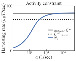
Activity constraint: analogously to Sec. II.3, we now define:
| (S2.59) |
for values of in units of . Solving (10) under yields the blue curve in Fig. S12 for as a function of .
Thermodynamic affinity constraint: owing to the same reasoning as in Sec. II.3, this constraint proves physically meaningful if combined with another constraint on the fluxes, such as the activity constraint (S2.59). In this case, we analogously define the feasibility set:
| (S2.60) |
In the inset of Fig. S12, we show the solution to (10) under for values of a range of with fixed values of (green line) and (red line).
III Closed-form solutions of Eq. (11) in different regimes
We consider a system of states indexed by that evolves according to a Markovian master equation with rate matrix , where and correspond to baseline and control processes respectively. Here we study the optimization (11) in three limiting regimes.
III.1 Linear Response (LR) regime, Eq. (15)
We first consider (11) in the linear response regime, that is under the assumption that the optimal distribution is close to the baseline steady state , thereby arriving at (15). We assume that is irreducible and has a unique steady state with full support. Note that the assumption that has full support is satisfied when is “weakly reversible”, meaning that whenever .
First, we rewrite the entropic term in (13) as
| (S3.62) | ||||
| (S3.63) |
where in the last step we used that when is the steady-state distribution of the baseline. We focus on the first term in (S3.63), and use the expansion for , to derive
| (S3.64) |
where we defined
| (S3.65) |
Our variable to optimize is a probability distribution , which needs to satisfy two constrains: and . The latter constraint holds automatically, given our hypothesis that is very close to . The former constraint can be expressed in terms of by setting
| (S3.66) |
We impose this linear constraint on below, when redefining the optimization problem in terms of rather than .
Before we finish off with the entropic term, we introduce the following symmetric matrix:
| (S3.67) |
The matrix is sometimes dubbed the “additive symmetrization” of . It will always obey the detailed balance condition (DB) for , . Moreover, if and only if obeys DB. We note that only in this latter case would be an equilibrium distribution. We also define:
| (S3.68) |
Observe that , which implies that and are related via a similarity transformation so any right eigenpair of , is an eigenpair of the symmetric matrix . Also, since and are both symmetric, so is . In particular, since is the sum of two irreducible rate matrices, it is then itself an irreducible rate matrix which has a unique right eigenvector. It is easy to show that, in fact, is ’s steady-state distribution with eigenvalue . Then, by similarity, also has a unique eigenvector with eigenvalue . Moreover, since is a rate matrix, it is negative semidefinite (), and so is also negative semidefinite. We indicate the right eigenvectors of as and the eigenvectors of the symmetric matrix as . We assume that are normalized as , therefore .
Going back to (S3.64), we note that
| (S3.69) |
In order to keep track of the second term in (S3.63), let us first recall the free-energy term in (13) and the pay-off vector which, in terms of the baseline parameters, reads as
and conveniently redefine it such that:
| (S3.70) |
For reasons that will become obvious below, we re-scale (S3.70) by setting
| (S3.71) |
We combine the above with the definition (S3.65) and the nonlinear term (S3.69). We then recast the optimization problem in terms of the variable , which is constrained by (S3.66). Finally, under the LR regime, (11) is approximated by
| (S3.72) |
Eq. (S3.72) is a quadratic optimization problem, which can be solved using standard techniques from linear algebra. For convenience we summarize these techniques in Lemma 1 in Sec. V of this SM. That theorem implies that
| (S3.73) |
where is the Moore-Penrose pseudo-inverse of . In applying Theorem 1, we used result (S5.123) and the relation , where solves (S3.72).
We can rewrite (S3.73) using the eigensystem of ,
| (S3.74) |
Finally, as in the main text we define
| (S3.75) |
which can be interpreted as the harvesting amplitude of the eigenmodes of . Plugging into (S3.73) gives Eq. (15) in the main text,
| (S3.76) |
Region of validity of the LR regime
Note that the LR regime applies when . We can write
| (S3.77) |
where we used the triangle inequality and properties of the matrix norm. Therefore, the LR approximation is guaranteed to be valid when
| (S3.78) |
In other words, the harvesting amplitude on each eigenmode must be slower than relaxation modes, up to a factor that depends only on , , and the steady state .
III.2 Deterministic (D) regime, Eq. (16)
In the Deterministic (D) regime, we assume that the nonlinear terms in (13) are small compared to the linear terms. This allows us to approximate the optimal solution of (13) as the linear optimization
| (S3.79) | ||||
| (S3.80) |
where . The maximum in (S3.80) is achieved by with , so
| (S3.81) |
as appears in the main text.
Region of validity of the D regime
We now discuss when the Deterministic regime approximation is valid.
We begin by making the assumption that the baseline harvesting rate is non-negative, . In addition, for notational convenience, let indicate the largest escape rate.
We express the regime of validity in terms of the following two parameters:
| (S3.82) | ||||
| (S3.83) |
The parameter reflects the balance between diffusion out of the optimal state versus Deterministic harvesting rate. The parameter is the minimal steady-state probability of any state.
Assuming , we show that
| (S3.84) |
The RHS of (S3.84) vanishes for , so the LHS tightens as . We emphasize that the D approximation only becomes accurate in relative, not additive, terms (i.e., it is not necessarily true that ).
To derive (S3.84), we first consider an upper bound on . Observe that for any ,
| (S3.85) |
where we used for and . Plugging into (S3.79) and using that for all and , we then have
| (S3.86) |
To derive a lower bound on , define the distribution , with as in (S3.82). Plugging this distribution into the objective in (S3.79) yields
| (S3.87) |
where we used that since . Using , we bound the first term on the right side of (S3.87) as
| (S3.88) |
where we used that in the last inequality. For the second term on the right side of (S3.87),
| (S3.89) |
We can plug (III.2) and (S3.89) into (S3.87) to give a lower bound on ,
where we used the definition of (S3.82) and rearranged. Since , we can further drop the term to give
| (S3.90) |
where in the second line we used the assumption . Combining and using that yields
| (S3.91) |
which can be rearranged to give (S3.84).
Interestingly, we can also derive a relative perturbation bound on the maximum increase of the harvesting rate, above the baseline harvesting rate. Specifically, using a similar derivation as above, we can show that
| (S3.92) |
where and is defined as before. In fact, this perturbation bound on the increase holds without any additional assumptions, i.e., regardless of the sign of .
III.3 Near-Deterministic (ND) regime, Eq. (17)
In this regime, we consider a perturbation of the Deterministic regime: we assume that the optimal is close to a delta-function distribution centered at . If ,
| (S3.93) |
This allows us to approximate the entropic term in (S3.79) as
| (S3.94) |
where we used when . Plugging into (S3.79) gives
| (S3.95) |
where we recall that , which does not depend on . After maximizing with respect to by taking derivatives and setting them to zero, one obtains
| (S3.96) |
Plugging (S3.96) into (III.3) gives
| (S3.97) |
Region of validity of the ND regime
The ND approximation applies when , or equivalently when
For convenience, we define the harvesting gap as the difference in the pay-off between the optimal state and the second optimal state,
By combining and rearranging the above, we can simplify the validity condition for the ND approximation as
| (S3.98) |
Note that this condition also guarantees that for . Expression (S3.98) implies that ND approximation is valid when the harvesting gap is much larger than the rates of escape from the optimal state .
IV Unicyclic model
Here we analyze the unicyclic model considered in the main text. Before proceeding, we briefly introduce some useful facts about the eigendecomposition of a unicylic rate matrix.
IV.1 An Algebraic Aperitif: eigendecomposition of unicyclic rate matrix
Consider a unicylic rate matrix ,
| (S4.99) |
which is a symmetric circulant matrix. Due to symmetry, its steady state is uniform: for all . The eigensystem for is obtained from the theory of circulant matrices [45], which, for odd , yields:
| (S4.100) |
where . These eigenvalues are all degenerate twice (except , whose eigenvector is simply ). An orthonormal choice of eigenbasis is given by the set
| (S4.101) |
IV.2 Transition harvesting cycle
We now analyze the unicyclic model using techniques developed in Sec. III. We consider a systems with state arranged in a ring, where baseline transitions are symmetric with uniform kinetics: , (see Fig. S13 here and Fig. 4 (a) in the main text). The baseline dynamics are equivalent to a random walk on a one-dimensional ring, and the baseline rate matrix is given by (S4.99).
We assume that a single transition, taken to be without loss of generality, harvests joules of free energy. In addition, note that in the main text we chose to set the units of without loss of generality. However, we have kept explicit in the rest of the SM. For this system, the baseline steady state is uniform, , and the harvesting vector is
| (S4.102) |

In the rest of this section, we analyze this model in the LR, D and ND regimes. We will also discuss the validity of these approximation in terms of the model parameters.
IV.2.1 LR regime
We first consider the LR solution (S3.76). Combining (S4.102) with (S3.71), , and gives . In addition, since in this particular example obeys detailed balance, . Finally, it is easy to verify that . Thus, has the same eigendecomposition as . The normalized eigenvectors of are given by (S4.101).
We can compute for , using the eigenvector set given in (S4.101),which simply yields
| (S4.103) |
Next, we compute the maximum harvesting rate attainable using (S3.76),
| (S4.104) |
On the other hand, continuing with odd , it is also possible to compute the deviation of the optimal distribution from stationary distribution using (S3.76),
| (S4.105) |
which is depicted in Fig. S14(a). (Note that, due to our choice of a complex-valued eigenbasis, we must be careful in adding the complex conjugate on the , following the ordering of the operator in (S3.76).) Now, component by component, we can rewrite (S4.105) as
| (S4.106) |
In the first line, we used the expressions for from (S4.103), from (S4.100), from (S4.101), and and then simplified. In the second line, we expanded into real and imaginary components and then used that the imaginary components cancel over the sum. In the last line, we used the identity for and and then simplified. It can be verified that the first series in (S4.106) sums to . The second series is trickier but can be simplified using trigonometric methods as shown in Ref. [79]. Plugging in that solution and simplifying gives the very simple expression:
| (S4.107) |
Thus, in the LR regime, the optimal distribution builds up in equal increments starting at until the optimal state , after which it falls off a cliff. This is shown in Fig. S14.

We can also compute the probability current across the transition , which we leave as an exercise for the reader:
| (S4.108) |
The expressions (S3.77) and (S3.78) suggest for which values of the optimal solution will be in the LR regime. In this case, however, it is possible to work out the norm exactly:
which implies that the LR regime is valid when
| (S4.109) |
In this case, the larger the number of states in the ring, the wider the interval of values that will make the optimal solution fall into the LR regime. For large , we obtain
IV.2.2 D and ND Regimes
Note that the optimal mesostate is . Hence and . Next, consider the ND expressions (S3.96) with the payoff vector (S4.102). Denote and ; and observe that , and for all . Hence, for , we obtain
| (S4.110) |
The harvesting rate attainable in this regime can be calculated using Eq. (S3.97),
| (S4.111) | ||||
| (S4.112) |
IV.3 State harvesting cycle
In this section, we consider the second unicyclic model, see Fig. S15 and Fig. 4 (b) in the main text. In this model, the baseline dynamics correspond once again to the unicycle with symmetric rates, as in Sec. IV.2. However, harvesting is not coupled to transitions, but rather to internal fluxes within a single mesostate. Without loss of generality, we choose this mesostate to be . In other words, we let and . There is now no preferential direction for the probability current. The free energy harvested per unit time when the system is in mesostate is given by the parameter , which carries the same units as . Just as before, the baseline steady state is uniform, i.e. . Hence, the harvesting vector is
| (S4.113) |
Below we consider the LR, D and ND regimes.
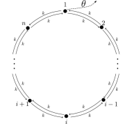
IV.3.1 LR Regime
In analogy with the previous example, the expression for the upper bound in free energy harvesting rate under the LR regime here is obtained as
| (S4.114) |
with , where the vectors correspond to the eigensystem discussed in discussed in Sec. IV.1, i.e. in (S4.101). On the other hand, here . The latter is obtained by construction using (S3.65), (S3.70) and (S3.71). Thus,
For large even , it is possible to show that [80]
| (S4.115) |
which allows us to write
| (S4.116) |
If we wanted to approximate the result above for a large odd , we would need to add a term proportional to , which is of second order, hence the leading order is still captured by expression (S4.116).
We can also study the optimal distribution using (S3.76),
| (S4.117) |
with . This is computed numerically and its behavior is shown in Fig. S14(b). We leave this computation as an exercise to the reader.

Expression (S3.78) suggests sufficiency conditions for when the optimum will be in the LR regime. Note that, in this case, while
Then, using , condition (S3.78) will read as:
| (S4.118) |
For sufficiently large , we can approximate , so the LR regime is valid when
| (S4.119) |
Expression (S3.78), however, is not necessarily a tight bound. That is, the result hereby obtained is a sufficient condition for the LR regime to be valid, but not a necessary one.
IV.3.2 D and ND Regimes
The optimal mesostate is . Hence
Next, by following a similar procedure as above, we denote , , and for all . Thus, for , we obtain:
| (S4.120) |
The harvesting rate attainable in this regime can be calculated using Eq. (S3.97),
| (S4.121) |
V Quadratic optimization lemma
In this section, we provide a useful theorem for solving the quadratic optimization problems that occurs in our analysis of the linear response (LR) regime. It uses standard techniques from linear algebra.
Lemma 1.
Consider the maximization problem
| (S5.122) |
where is a negative semidefinite symmetric matrix with a single null eigenvector and is any vector. The solution is given by:
| (S5.123) |
where is the Moore-Penrose pseudo-inverse of .
Proof.
Since is symmetric, its real valued eigendecomposition can be written as:
where we will choose , without loss of generality, i.e. is the only zero eigenvalue. The Moore-Penrose pseudo-inverse of can be written as:
The constraint on the optimization problem reads as , which implies that
Now, consider the objective function,
| (S5.124) |
where we used properties of the transverse operation, symmetry of and , that , and that . Note that the last term on the right hand side of the previous expression does not depend on , and that the first term is always non-positive because is negative semidefinite. Thus, the objective is maximized only by setting the first term to zero, which is achieved by . Upon substitution, this yields .
∎