Optimized Power Control for Over-the-Air Federated Edge Learning
Abstract
Over-the-air federated edge learning (Air-FEEL) is a communication-efficient solution for privacy-preserving distributed learning over wireless networks. Air-FEEL allows “one-shot” over-the-air aggregation of gradient/model-updates by exploiting the waveform superposition property of wireless channels, and thus promises an extremely low aggregation latency that is independent of the network size. However, such communication efficiency may come at a cost of learning performance degradation due to the aggregation error caused by the non-uniform channel fading over devices and noise perturbation. Prior work adopted channel inversion power control (or its variants) to reduce the aggregation error by aligning the channel gains, which, however, could be highly suboptimal in deep fading scenarios due to the noise amplification. To overcome this issue, we investigate the power control optimization for enhancing the learning performance of Air-FEEL. Towards this end, we first analyze the convergence behavior of the Air-FEEL by deriving the optimality gap of the loss-function under any given power control policy. Then we optimize the power control to minimize the optimality gap for accelerating convergence, subject to a set of average and maximum power constraints at edge devices. The problem is generally non-convex and challenging to solve due to the coupling of power control variables over different devices and iterations. To tackle this challenge, we develop an efficient algorithm by jointly exploiting the successive convex approximation (SCA) and trust region methods. Numerical results show that the optimized power control policy achieves significantly faster convergence than the benchmark policies such as channel inversion and uniform power transmission.
I Introduction
In the pursuit of ubiquitous intelligence envisioned in the future 6G networks, recent years have witnessed the spreading of artificial intelligence (AI) algorithms from the cloud to the network edge, resulting in an active area called edge intelligence [1, 2]. The core research issue therein is to allow low-latency and privacy-aware access to rich mobile data for intelligence distillation. To this end, a popular framework called federated edge learning (FEEL) is proposed recently, which distributes the task of model training over edge devices so as to reduce the communication overhead and keep the data-use locally [3, 4]. Essentially, the FEEL framework is a distributed implementation of stochastic gradient decent (SGD) over wireless networks. A typical training process involves iterations between 1) broadcasting of the global model under training from edge server to devices for local SGD execution using local data, and 2) local models/gradients uploading from devices to edge server for aggregation and global model updating. Although the uploading of high-volume raw data is avoided, the updates aggregation process in FEEL may still suffer from a communication bottleneck due to the high-dimensionality of each updates and the multiple access by many devices over wireless links. To tackle this issue, one promising solution called over-the-air FEEL (Air-FEEL) has been proposed, which exploits the over-the-air computation (AirComp) for “one-shot” aggregation via concurrent update transmission, such that communication and computation are integrated in a joint design by exploiting the superposition property of a multiple access channel (MAC) [1, 5, 6].
The idea of AirComp was first proposed in [5] in the context of data aggregation in sensor networks, where it is surprisingly found that “interference” can be harnessed by structured codes to help functional computation over a MAC. Inspired by the finding, it was shown in the subsequent work [6] that for Gaussian independent and identically distributed (i.i.d.) data sources, the uncoded transmission is optimal in terms of distortion minimization. Besides the information-theoretic studies, various practical issues faced by AirComp implementation were also considered in [7, 8, 9]. In particular, the synchronization issue in AirComp was addressed in [7] via an innovative idea of shared clock broadcasting from edge server to devices. The optimal power control policies for AirComp over fading channels were derived in [8] to minimize the average computation distortion, and the cooperative interference management framework for coordinating coexisting AirComp tasks over multi-cell networks was developed in [9].
More recently, AirComp found its merits in the new context of FEEL, known as Air-FEEL, for communication-efficient update aggregation as demonstrated in a rich set of prior works [10, 11, 12, 13, 14, 15]. Specifically, a broadband Air-FEEL solution was proposed in [10], where several communication-learning tradeoffs were derived to guide the design of device scheduling. Around the same time, a source-coding algorithm exploiting gradient sparsification was proposed in [11] to implement Air-FEEL with compressed updates for higher communication efficiency. In parallel, a joint design of device scheduling and beamforming in a multi-antenna system was presented in [12] to accelerate Air-FEEL. Subsequently, the gradient statistics aware power control was investigated in [13] to further enhance the performance of Air-FEEL. Furthermore, to allow Air-FEEL compatible with digital chips embedded in modern edge devices, Air-FEEL based on digital modulation was proposed in [14] featuring one-bit quantization and modulation at the edge devices and majority-vote based decoding at the edge server. Besides the benefit of low latency, Air-FEEL was also found to be beneficial in data privacy enhancement as individual updates are not accessible by edge server, eliminating the risk of model inversion attack [15].
Despite the promise in high communication efficiency, Air-FEEL may suffer from severe learning performance degradation due to the aggregation error caused by the non-uniform channel fading over devices and noise perturbation. Prior work in this field mostly assumed channel inversion power control (or its variants) [10, 11, 12, 15] in an effort to reducing the aggregation error by aligning the channel gains, which could be highly suboptimal in deep fading scenarios due to the noise amplification. Although there exists one relevant study on power control for Air-FEEL system in [13], it focused on the minimization of the intermediate aggregation distortion (e.g., mean squared error) instead of the ultimate learning performance (e.g., the general loss function). Therefore, there still leaves a research gap in learning performance optimization of Air-FEEL by judicious power control, motivating the current work. To close the gap, we first analyze the convergence behavior of the Air-FEEL by deriving the optimality gap of the loss-function under arbitrary power control policy. Then the power control problem is formulated to minimize the optimality gap for convergence acceleration, subject to a set of average and maximum power constraints at edge devices. The problem is generally non-convex and challenging to solve due to the coupling of power control variables over different devices and iterations. The challenge is tackled by the joint use of successive convex approximation (SCA) and trust region methods in the optimized power control algorithm derivation. Numerical results show that the optimized power control policy achieves significantly faster convergence than the benchmark policies such as channel inversion and uniform power transmission, thus opening up a new degree-of-freedom for regulating the performance of Air-FEEL by power control.
II System Model
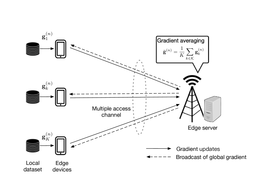
We consider an Air-FEEL system consisting of an edge server and edge devices, as shown in Fig. 1. With the coordination of the edge server, the edge devices cooperatively train a shared machine learning model via over-the-air update aggregation as elaborated in the sequel.
II-A Learning Model
We assume that the learning model is represented by the parameter vector with denoting the model size. Let denote the local dataset at edge device , in which the -th sample and its ground-true label are denoted by and , respectively. Then the local loss function of the model vector on is
| (1) |
where denotes the sample-wise loss function quantifying the prediction error of the model on the sample with respect to (w.r.t.) its ground-true label , and denotes the strongly convex regularization function scaled by a hyperparameter . For notational convenience, we simplify as . Then, the global loss function on all the distributed datasets is given by
| (2) |
where with , and the sizes of datasets in all edge devices are assumed to be uniform for notation simplicity, i.e., .
The objective of the training process is to minimize the global loss function :
| (3) |
Instead of directly uploading all the local data to the edge server for centralized training, the learning process in (3) can be implemented iteratively in a distributed manner based on gradient-averaging approach as illustrated in Fig. 1.
At each communication round , the machine learning model is denoted by . Then each edge device can compute the local gradient denoted by using the local dataset :
| (4) |
where is the gradient operator and we assume that the whole local dataset is used to estimate the local gradients. Next, the edge devices upload all local gradients to the edge server, which are further averaged to obtain the global gradient:
| (5) |
Then, the global gradient estimate is broadcast from edge server to edge devices, based on which edge device can update its own model under training via
| (6) |
where is the learning rate. Notice that the above procedure continues until convergence criteria is met or the maximum number of iterations is achieved.
II-B Basic Assumptions on Learning Model
To facilitate the convergence analysis next, we make several standard assumptions on the loss function and gradient estimates.
Assumption 1 (Smoothness).
Let denote the gradient of the loss function evaluated at point . Then there exists a non-negative constant vector , such that
where the superscript denotes the transpose operation.
Assumption 2 (Polyak-Lojasiewicz Inequality).
Let denote the optimal loss function value to problem (3). There exists a constant such that the global loss function satisfies the following Polyak-Lojasiewicz (PL) condition:
Notice that the above assumption is more general than the standard assumption of strong convexity [16]. Typical loss functions that satisfy the above two assumptions include logistic regression, linear regression and least squares.
Assumption 3 (Variance Bound).
The local gradient estimates , defined in (4), where the index is omitted for simplicity, are assumed to be independent and unbiased estimates of the batch gradient with coordinate bounded variance, i.e.,
| (7) | |||
| (8) |
where and are defined as the -th element of and , respectively, and is a vector of non-negative constants.
II-C Communication Model
The distributed training latency is dominated by the update aggregation process, especially when the number of devices becomes large. Therefore, we focus on the aggregation process over a MAC. Instead of treating different devices’ update as interference, we consider AirComp for fast update aggregation by exploiting the superposition property of MAC. We assume that the channel coefficients remain unchanged within a communication round, and may change over different communication rounds. Besides, the channel state information (CSI) is assumed to be available at all edge devices, so that they can perfectly compensate for the phases introduced by the wireless channels.
Let denote the complex channel coefficient from device to the edge server at communication round , and denote its magnitude with . During the gradient-uploading phase, all the devices transmit simultaneously over the same time-frequency block, and thus the received aggregate signal is given by
| (9) |
in which denotes the transmit power at device , and denotes the additive white Gaussian noise with , where is the noise power density and is an identity matrix. Therefore, the global gradient estimate at the edge server is given by
| (10) |
The devices can adaptively adjust their transmit powers for enhancing the learning performance. In practice, the transmit power of each edge device at each communication round is constrained by a maximum power budget :
| (11) |
In addition, each device is also constrained by an average power budget denoted by over the whole training period as expressed below:
| (12) |
Here, we generally have .
III Convergence Analysis for Air-FEEL with Adaptive Power Control
In this section, we formally characterize the learning performance of Air-FEEL system, which is derived to be a function of transmit powers of all devices.
Let denote the number of needed communication rounds and . For notational convenience, we use to represent . The optimality gap after communication rounds defined by is derived in the following theorem, from which we can understand the convergence behavior of Air-FEEL.
Theorem 1 (Optimality Gap).
The optimality gap for Air-FEEL, with arbitrary transmit power control policy , is given as
| (13) |
with and .
Proof:
The proof follows the widely-adopted strategy of relating the norm of the gradient to the expected improvement made in a single algorithmic step, and comparing this with the total possible improvement.
where the inequalities (a) and (b) follows the Assumption 1 and . By subtracting and taking expectation at both sides, the convergence rate of each communication round is given by (14). Next, (15) is obtained by applying the PL condition in the Assumption 2. Then, by applying above inequality repeatedly through iterations, after some simple algebraic manipulation we have (13), which completes the proof.
| (14) |
| (15) |
∎
Further applying the mean inequality , we can derive a more elegant upper bound for the expression in (13) to attain more insights as follows
| (16) |
where and for while .
Remark 1.
The first term on the right hand side of (16) suggests that the effect of initial optimality gap vanishes as the number of communication round increases. The second term reflects the impact of the power control and additive noise power on the convergence process, that is, transmission with more power in the initial learning iterations is more beneficial in decreasing the optimality gap. This is because that the contribution of power control at iteration is discounted by a factor .
IV Power Control Optimization
In this section, we focus on speeding up the convergence rate by minimizing the optimality gap in Theorem 1, under the power constraints stated in (11) and (12). The optimization problem is thus formulated as
Due to the coupling between the power control and learning rate , problem (P1) is non-convex and hard to solve. We resort to the alternating optimization technique for efficiently solving this problem. In particular, we first solve problem (P1) under any given , and then apply a one-dimension search to find the optimal that achieves the minimum objective value.
Let under any given . Note that the transmit powers at different devices and different communication rounds are coupled with each other in the objective function in (13) under given learning rate , leading to a highly non-convex problem:
To tackle this problem, we propose an iterative algorithm to obtain an efficient solution using the SCA technique. The key idea is that under any given local point at each iteration, we can approximate the non-convex objective as a constructed convex one. Therefore, after solving a series of approximate convex problems iteratively, we can obtain a high-quality suboptimal solution to problem (P2).
Let denote the local point at the -th iteration with , and the set of communication rounds. Notice that by checking the first-order Taylor expansion of w.r.t. at the local point , it follows that
where represents the first-order derivative w.r.t. , given in (17) and (18).
| (17) | ||||
| (18) |
In this case, is linear w.r.t. . To ensure the approximation accuracy, a series of trust region constraints are imposed as [17]
| (19) |
where denotes the radius of the trust region. By replacing as the approximation of and introducing an auxiliary variable , the approximated problem at the -th iteration is derived as a convex problem:
| (20) | ||||
which can be directly solved by CVX [18].
Let denote the optimal power control policy to problem (P2.1) at local point . Then, we can obtain an efficient iterative algorithm to solve problem (P2) as follows. In each iteration , the power control is updated as by solving problem (P2.1) at local point , i.e. , where denotes the initial power control. At the -th iteration, we compute the objective value in problem (P2) by replacing as . If the objective value decreases, we then replace the current point by the obtained solution and go to the next iteration; otherwise, we update and continue to solve problem (P2.1). This algorithm would stop until that is lower than a given threshold denoted by . In summary, the proposed algorithm is presented in Algorithm 1.
Algorithm 1 for Solving Problem (P2)
-
1
Initialization: Given the initial power control ; let .
-
2
Repeat:
-
a)
Solve problem (P1.1) under given to obtain the optimal solution as ;
-
b)
If the objective value of problem (P2) decreases, then update with ; otherwise ;
-
a)
-
3
Until .
With the obtained power control in Algorithm 1, we can find the optimal accordingly via a one-dimensional search.
V Simulation Results
In this section, we provide simulation results to validate the performance of the proposed power control policy for Air-FEEL. In the simulation, the wireless channels from each device to the edge server over fading states follow i.i.d. Rayleigh fading, such that ’s are modeled as i.i.d. circularly symmetric complex Gaussian (CSCG) random variables with zero mean and unit variance. The dataset with size at all device are randomly generated, where part of the data, namely pairs (, ), are left for prediction, and the remaining ones are used for model training. The generated data sample vector follow i.i.d. Gaussian distribution as and the label is obtained as , where represents the -entry in vector and is the observation noise with i.i.d. Gaussian distribution, i.e., . Unless stated otherwise, the data samples are evenly distributed among the devices, and thus it follows . Moreover, we apply ridge regression with the sample-wise loss function and the regularization function with in this paper. Furthermore, recall that and then we can obtain the smoothness parameter and PL parameter as the largest and smallest eigenvalues of the data Gramian matrix , in which is the data matrix. The optimal loss function is computed according to the optimal parameter vector to the learning problem (3), where with . We set the initial parameter vector as an all-zero vector and the noise variance .
We consider two benchmark schemes for performance comparison, namely the uniform power transmission that transmits with uniform power over different communication round under the constraint of average power budget, and the channel inversion adopted in [15]. As for the performance metric for comparison, we consider the optimality gap and prediction error to evaluate the learning performance.
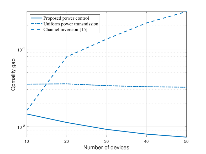
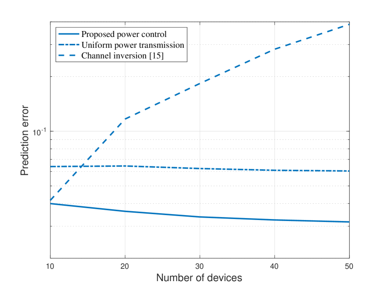
The effect of device population on learning performance is illustrated in Fig. 2 with , where the power budgets at all devices are identically set to be W and W. Notice that the increasing of device population may introduce both the positive and negative effects on the learning performance. The positive effect is that the training process can exploit more data, while the negative effect is the increased aggregation error raised by AirComp over more devices. As observed in Fig. 2, the positive effect can be cancelled or even overweighed by the negative effect when applying the channel inversion or uniform power control. The blessing of including more devices in Air-FEEL can dominate the curse it brings only when the power control is judiciously optimized, showing the crucial role of power control in determining the the learning performance of Air-FEEL.
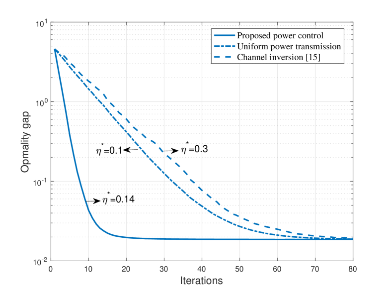
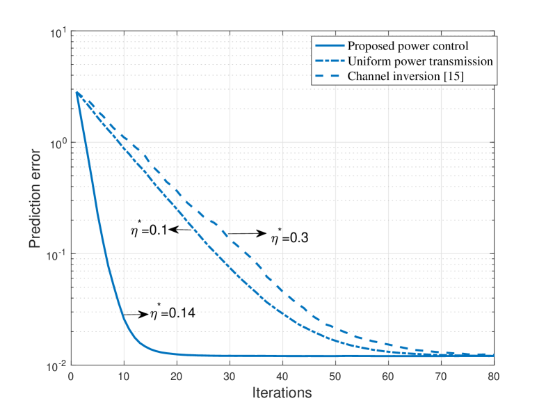
Fig. 3 shows the learning performance during the learning process under the optimized learning rate, where we set , W, W, and . It is observed that the proposed power control scheme can achieve faster convergence than both the channel-inversion and uniform-power-control schemes. This is attributed to the power control optimization directly targeting convergence acceleration.
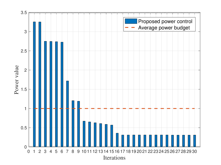
Fig. 4 shows the power allocation over a static channel with uniform channel gain during the learning process, where we set , W, W, and . It is observed that the power allocation over a static channel follows a stair-wise monotonously decreasing function. The behavior of power control coincides the analysis on Remark 1.
VI Conclusion
In this paper, we exploit power control as a new degree of freedom to optimize the learning performance of Air-FEEL, a promising communication-efficient solution towards edge intelligence. To this end, we first analyzed the convergence rate of the Air-FEEL by deriving the optimality gap of the loss-function under arbitrary power control policy. Then the formulated power control problem aimed to minimize the optimality gap for accelerating convergence, subject to a set of average and maximum power constraints at edge devices. Due to the coupling of power control variables over different devices and iterations, the challenge of the formulated power control problem was tackled by the joint use of SCA and trust region methods. Numerical results demonstrated that the optimized power control policy can achieve significantly faster convergence than the benchmark policies such as channel inversion and uniform power transmission.
References
- [1] G. Zhu, D. Liu, Y. Du, C. You, J. Zhang, and K. Huang, “Toward an intelligent edge: Wireless communication meets machine learning,” IEEE Commun. Mag., vol. 58, no. 1, pp. 19–25, Jan. 2020.
- [2] J. Park, S. Samarakoon, M. Bennis, and M. Debbah, “Wireless network intelligence at the edge,” Proc. IEEE, vol. 107, no. 11, pp. 2204–2239, Nov. 2019.
- [3] J. Konečný, H. B. McMahan, F. X. Yu, P. Richtárik, A. T. Suresh, and D. Bacon, “Federated learning: Strategies for improving communication efficiency,” 2016. [Online]. Available: https://arxiv.org/pdf/1610.05492.pdf
- [4] M. Chen, Z. Yang, W. Saad, C. Yin, H. V. Poor, and S. Cui, “A joint learning and communications framework for federated learning over wireless networks,” IEEE Trans. Wireless Commun., pp. 1–1, 2020.
- [5] B. Nazer and M. Gastpar, “Computation over multiple-access channels,” IEEE Trans. Inf. Theory, vol. 53, no. 10, pp. 3498–3516, Oct. 2007.
- [6] M. Gastpar, “Uncoded transmission is exactly optimal for a simple gaussian sensor network,” IEEE Trans. Inf. Theory, vol. 54, no. 11, pp. 5247–5251, Nov. 2008.
- [7] O. Abari, H. Rahul, D. Katabi, and M. Pant, “Airshare: Distributed coherent transmission made seamless,” in Proc. IEEE INFOCOM, Kowloon, Hong Kong, Apr. 2015, pp. 1742–1750.
- [8] X. Cao, G. Zhu, J. Xu, and K. Huang, “Optimized power control for over-the-air computation in fading channels,” IEEE Trans. Wireless Commun., pp. 1–1, 2020.
- [9] X. Cao, G. Zhu, J. Xu, and K. Huang, “Cooperative interference management for over-the-air computation networks,” 2020. [Online]. Available: https://arxiv.org/pdf/2007.11765.pdf
- [10] G. Zhu, Y. Wang, and K. Huang, “Broadband analog aggregation for low-latency federated edge learning,” IEEE Trans. Wireless Commun., vol. 19, no. 1, pp. 491–506, Jan. 2020.
- [11] M. Mohammadi Amiri and D. Gunduz, “Machine learning at the wireless edge: Distributed stochastic gradient descent over-the-air,” IEEE Trans. Signal Process., vol. 68, pp. 2155–2169, 2020.
- [12] K. Yang, T. Jiang, Y. Shi, and Z. Ding, “Federated learning via over-the-air computation,” IEEE Trans. Wireless Commun., vol. 19, no. 3, pp. 2022–2035, Mar. 2020.
- [13] N. Zhang and M. Tao, “Gradient statistics aware power control for over-the-air federated learning,” 2020. [Online]. Available: https://arxiv.org/pdf/2003.02089.pdf
- [14] G. Zhu, Y. Du, D. Gunduz, and K. Huang, “One-bit over-the-air aggregation for communication-efficient federated edge learning: Design and convergence analysis,” 2020. [Online]. Available: https://arxiv.org/pdf/2001.05713.pdf
- [15] D. Liu and O. Simeone, “Privacy for free: Wireless federated learning via uncoded transmission with adaptive power control,” 2020. [Online]. Available: https://arxiv.org/pdf/2006.05459.pdf
- [16] H. Karimi, J. Nutini, and M. Schmidt, “Linear convergence of gradient and proximal-gradient methods under the polyak-łojasiewicz condition,” Lecture Notes in Computer Science, pp. 795–811, 2016. [Online]. Available: http://dx.doi.org/10.1007/978-3-319-46128-1_50
- [17] B. Dai, Y. Liu, and W. Yu, “Optimized base-station cache allocation for cloud radio access network with multicast backhaul,” IEEE J. Sel. Areas Commun., vol. 36, no. 8, pp. 1737–1750, Aug. 2018.
- [18] M. Grant and S. Boyd, “CVX: Matlab software for disciplined convex programming,” 2016. [Online]. Available: http://cvxr.com/cvx