Optimized Schwarz waveform relaxation and discontinuous Galerkin time stepping for heterogeneous problems.
Abstract
We design and analyze Schwarz waveform relaxation algorithms for domain decomposition of advection-diffusion-reaction problems with strong heterogeneities. These algorithms rely on optimized Robin or Ventcell transmission conditions, and can be used with curved interfaces. We analyze the semi-discretization in time with discontinuous Galerkin as well. We also show two-dimensional numerical results using generalized mortar finite elements in space.
keywords:
Coupling heterogeneous problems, domain decomposition, optimized Schwarz waveform relaxation, time discontinuous Galerkin, nonconforming grids, error analysis.AMS:
65 M 15, 65M50, 65M55.1 Introduction
In many fields of applications such as reactive transport, far field simulations of underground nuclear waste disposal or ocean-atmosphere coupling, models have to be coupled in different spatial zones, with very different space and time scales and possible complex geometries. For such problems with long time computations, a splitting of the time interval into windows is essential, with the possibility to use robust and fast solvers in each time window.
The Optimized Schwarz Waveform Relaxation (OSWR) method was introduced for linear parabolic and hyperbolic problems with constant coefficients in [4]. It was analyzed for advection diffusion equations, and applied to non constant advection, in [17]. The algorithm computes independently in each subdomain over the whole time interval, exchanging space-time boundary data through optimized transmission operators. The operators are of Robin or Ventcell type, with coefficients optimizing a convergence factor, extending the strategy developed by F. Nataf and coauthors [3, 12]. The optimization problem was analyzed in [5], [1].
This method potentially applies to different space-time discretization in subdomains, possibly nonconforming and needs a very small number of iterations to converge. Numerical evidences of the performance of the method with variable smooth coefficients were given in [17]. An extension to discontinuous coefficients was introduced in [6], with asymptotically optimized Robin transmission conditions in some particular cases.
The discontinuous Galerkin finite element method in time offers many advantages. Rigorous analysis can be made for any degree of accuracy and local time-stepping, and time steps can be adaptively controlled by a posteriori error analysis, see [20, 14, 16]. In a series of presentations in the regular domain decomposition meeting we presented the DG-OSWR method, using discontinuous Galerkin for the time discretization of the OSWR. In [2], [9], we introduced the algorithm in one dimension with discontinuous coefficients. In [10], we extended the method to the two dimensional case. For the space discretization, we extended numerically the nonconforming approach in [8] to advection-diffusion problems and optimized order 2 transmission conditions, to allow for non-matching grids in time and space on the boundary. The space-time projections between subdomains were computed with an optimal projection algorithm without any additional grid, as in [8]. Two dimensional simulations were presented. In [11] we extended the proof of convergence of the OSWR algorithm to nonoverlapping subdomains with curved interfaces. Only sketches of proofs were presented.
The present paper intends to give a full and self-contained account of the method for the advection diffusion reaction equation with non constant coefficients.
In Section 2, we present the Robin and Ventcell algorithms at the continuous level in any dimension, and give in details the new proofs of convergence of the algorithms for nonoverlapping subdomains with curved interfaces.
Then in Section 3, we discretize in time with discontinuous Galerkin, and prove the convergence of the semi-discrete algorithms for flat interfaces. Error estimates are derived from the classical ones [20].
The fully discrete problem is introduced in Section 4, using finite elements. The interfaces are treated by a new cement approach, extending the method in [8]. Given the length of the paper, the numerical analysis will be treated in a forthcoming paper.
We finally present in Section 5 simulations for two subdomains, with piecewise smooth coefficients and a curved interface, for which no error estimates are available. We also include an application to the porous media equation.
Consider the advection-diffusion-reaction equation in
| (1.1) |
with initial condition
| (1.2) |
The advection and diffusion coefficients and , as well as the reaction coefficient , are piecewise smooth, the problem is parabolic, i.e. a.e. in .
Theorem 1 (Well-posedness and regularity, [15]).
We consider now a decomposition of into nonoverlapping subdomains , as depicted in Figure 1. In all cases the boundaries between the subdomains are supposed to be hyperplanes at infinity.
| \psfrag{Oj}{$\Omega_{i}$}\includegraphics[width=73.7146pt]{subdomains.eps} | \psfrag{Oj}{$\Omega_{i}$}\includegraphics[width=60.70653pt]{subdomainsband.eps} |
Problem (1.1) is equivalent to solving problems in subdomains , with transmission conditions on the interface between two neighboring subdomains and , given by the jumps , . Here is the unit exterior normal to . As coefficients and are possibly discontinuous on the interface, we note, for , . The same notation holds for and .
To any , we associate the set of indices of the neighbors of .
Following [3, 4, 6], we propose as preconditioner for (1.1, 1.2), the sequence of problems
| (1.3a) | |||
| (1.3b) | |||
The boundary operators , acting on the part of the boundary of shared by the boundary of are given by
| (1.4) |
and are respectively the gradient and divergence operators on . are functions in and is in . The initial value is that of in each subdomain. An initial guess is given on for . By convention for the first iterate, the right-hand side in (1.3) is given by . Under regularity assumptions, solving (1.1) is equivalent to solving
| (1.5) |
for with the restriction of to .
2 Studying the algorithm for the P.D.E
The first step of the study is to give a frame for the definition of the iterates.
2.1 The local problem
The optimized Schwarz waveform relaxation algorithm relies on the resolution of the following initial boundary value problem in a domain with boundary :
| (2.1) |
where is the exterior unit normal to . The boundary operator is defined on by
| (2.2) |
The domain has either form depicted in Figure 1, left for , right otherwise.
The functions and are in , and is in . Either , and the boundary condition is of Robin type, or we suppose and the operator will be referred to as Order 2 or Ventcell operator. In the latter case, we need the spaces
| (2.3) |
which are defined for , and equipped with the scalar product
| (2.4) |
We define the bilinear forms on and on by
| (2.5) |
and
| (2.6) |
By the Green’s formula, we can write a variational formulation of (2.1):
| (2.7) |
The well-posedness is a generalization of results in [5, 1, 19]. It relies on energy estimates and Grönwall’s lemma.
Theorem 2.
Suppose , , , , , with a.e.
If , if is in , is in and is in , satisfying the compatibility condition , the subdomain problem (2.1) has a unique solution in .
If , if is in , is in , and is in , problem (2.1) has a unique solution in with .
Proof.
The existence result relies on a Galerkin method like in [18, 19]. In the sequel, denote positive real numbers depending only on the coefficients and the geometry. The basic estimate is obtained by multiplying the equation by and integrating by parts in the domain. We set and .
With the assumptions on the coefficients, we have
Case .
the last inequality coming from the trace theorem
| (2.8) |
We obtain with the Cauchy-Schwarz inequality
We now have with Grönwall’s lemma
| (2.9) |
We apply (2.9) to :
Thanks to the compatibility condition, can be estimated, using the equation, by , and we obtain
Case a.e.
and by the Cauchy-Schwarz inequality
Collecting these inequalities, we obtain
We now integrate in time and use Grönwall’s lemma to obtain for any in
| (2.10) |
We apply (2.10) to :
We now use the equations at time 0 to estimate . From the equation in the domain, we deduce that
and from the boundary condition that
which gives altogether
| (2.11) |
We can now apply the Galerkin method. When , we work in , while if a.e we consider . This gives a unique solution . The regularity is obtained for by the usual regularity results for the Laplace equation with Neumann boundary condition, since
In the other case, we have that
2.2 Convergence analysis for Robin transmission conditions
We suppose here the coefficients to be zero everywhere. Given initial guess on for , the algorithm reduces in each subdomain to
| (2.12a) | |||
| (2.12b) | |||
The well-posedness for the boundary value problem in the previous section permits to define the sequence of iterates. We now consider the convergence of this sequence.
Theorem 3.
Proof.
By linearity, it is sufficient to prove that the sequence of iterates converges to zero if .
We multiply (2.12a) by , integrate on , and use the Green’s formula. We obtain
| (2.13) |
We use now
| (2.14) |
We replace the boundary term in (2.13), and integrate in time. Since the initial value vanishes, we have for any time ,
Since the coefficients are all bounded, the last term in the right-hand side can be handled by the trace theorem (2.8) to be canceled with the terms in the left-hand side like in the proof of Theorem 3. We further insert the transmission condition in the right-hand side:
We sum on the subdomains, and on the iterations, the boundary terms cancel out except the first and last ones, and we obtain for any ,
| (2.15) |
with
We now apply Grönwall’s lemma and obtain that for any ,
which proves that the sequence converges to zero in for each , and concludes the proof of the theorem. ∎
Remark 4.
In the case , if and , then in (2.15) and we conclude without using Grönwall’s lemma.
2.3 Order 2 transmission conditions
Theorem 5.
Proof.
We first need some results in differential geometry. For any , For every , the normal vector can be extended in a neighbourhood of in as a smooth function with length one. Let , such that in a neighbourhood of , in a neighbourhood of for and on . We can assume that is defined on a neighbourhood of the support of . We extend the tangential gradient and divergence operators in the support of by:
It is easy to see that , and for and with support in , we have
| (2.16) |
Now we prove Theorem 5. We consider the algorithm (1.3) on the error, so we suppose . We set , , , and .
The proof is based on energy estimates containing the term
and that we derive by multiplying successively the first equation of (1.3) by the terms , , and .
We multiply the first equation of (1.3) by , integrate on and integrate by parts in space,
| (2.17) |
We multiply the first equation of (1.3) by , integrate on and then integrate by parts in space,
| (2.18) |
We multiply the first equation of (1.3) by integrate on and integrate by parts in space:
| (2.19) |
We observe that
| (2.20) |
with
| (2.21) |
Replacing (2.21) in (2.20) and then (2.20) in (2.19), we obtain
| (2.22) |
Now we multiply the first equation of (1.3) by integrate on and integrate by parts in space:
| (2.23) |
We have,
| (2.24) |
Replacing (2.3) in (2.23) leads to
| (2.25) |
Multiplying (2.18), (2.22) and (2.25) by , and adding the three equations with (2.17), we get
We bound the right-hand side by
We simplify the terms which appear on both sides, and obtain
| (2.26) |
Recalling that on and on , we use now:
| (2.27) |
Replacing (2.27) into (2.26), we obtain
| (2.28) |
In order to estimate the fourth term in the right-hand side of (2.28), we observe that
By the trace theorem in the right-hand side, we write:
and
| (2.29) |
we obtain
| (2.30) |
Moreover, integrating by parts and using the trace theorem, we have
| (2.31) |
Using (2.29), we estimate the third term in the right-hand side of (2.28) by
| (2.32) |
Replacing (2.31), (2.30) and (2.32) in (2.28), then using the transmission conditions, we have:
We now sum up over the interfaces , then over the subdomains for , and on the iterations for , the boundary terms cancel out, and we obtain for any ,
| (2.33) |
with
| (2.34) |
We conclude with Grönwall’s lemma as before. ∎
3 The discontinous Galerkin time stepping for the Schwarz waveform relaxation algorithm
In the following sections, in order to simplify the analysis, we suppose that
a.e. in .
3.1 Time discretization of the local problem: discontinuous Galerkin method
We suppose that the coefficients are restricted to a.e. on , and a.e.. This implies that the bilinear form defined in (2.6) is positive definite on when , and positive definite on when a.e.
We recall the time-discontinuous Galerkin method, as presented in [14]. We are given a decomposition of the time interval , , for , the mesh size is . For a Banach space and an interval of , define for any integer
| (3.3) |
Let if , if . We define an approximation of , polynomial of degree lower than on every subinterval . For every point , we define , and note . The time discretization of (2.7) leads to searching such that
| (3.7) |
with . Since is closed at , is the value of at . Due to the discontinuous nature of the test and trial spaces, the method is an implicit time stepping scheme, and is obtained recursively on each subinterval, which makes it very flexible.
Theorem 6.
If a.e. on , and , equation (3.7) defines a unique solution.
Proof.
The result relies on the fact that the bilinear form is definite positive. It is is most easily seen by using a basis of Legendre polynomials. is obtained recursively on each subinterval. We introduce the Legendre polynomials , orthogonal basis in , with . has the parity of , hence . A basis of orthogonal polynomial on is given by . Choose in (3.7) with , and expand on as . Suppose to be given on . In order to determine on , we must solve the system: for any ,
It is an implicit scheme. We calculate the coefficients
which leads to
It is a square system of partial differential equations, of the type coercive compact. By the Fredholm alternative, we only need to prove uniqueness. Choose now , and obtain
and since is positive definite, we deduce that . ∎
We will make use of the following remark ([16]). We introduce the Gauss-Radau points, , defined such that the quadrature formula
is exact in , and the interpolation operator on at points . For any , .
Let be the operator whose restriction to each subinterval is and satisfies . By using the Gauss-Radau formula, which is exact in , we have for all
As a consequence, we have a very useful inequality:
| (3.8) |
Also, equation (3.7) can be rewritten as
| (3.9) |
or in the strong formulation:
| (3.10) |
Here is the projection in each subinterval of on .
3.2 The discrete in time optimized Schwarz waveform relaxation algorithm with different subdomains grids
In this part we present and analyse the discrete non conforming in time optimized Schwarz waveform relaxation method.
The time partition in subdomain , is , with intervals , and mesh size . In view of formulation (3.10), we define interpolation operators and projection operators in each subdomain, i.e. is the projection in each subinterval of on , and we solve
| (3.12a) | |||
| (3.12b) | |||
Here the operators are different on either part of the "equal" sign:
| (3.13) |
Formally, the sequence of problems (3.12) converges to the solution of
| (3.14a) | |||
| (3.14b) | |||
We present the analysis first with Robin transmission conditions (e.g. ) and general decomposition, and then with order 2 transmission conditions and decomposition in strips.
3.2.1 The Robin case
We consider here a general decomposition of the domain, possibly with corners. We solve (3.12) with , i.e. .
Theorem 8.
Proof.
We first write energy estimates on (3.12) for and . We start like in the proof of Theorem 3. We multiply (3.12a) by , integrate on , then integrate on the interval and use (3.8) and (2.14):
We can not use Grönwall’s Lemma like in the continuous case, due to the presence of the global in time projection operator in the transmission conditions. Therefore we have to assume that everywhere, which cancels the last term. We sum up over the time intervals, using the fact that the errors vanish at time 0:
We now insert the transmission conditions
We use the fact that the projection operator is a contraction to obtain:
We sum up over the subdomains, we define the boundary term
we obtain
| (3.15) |
We first apply this inequality to prove the first part of the Theorem. (3.14) is a square discrete system, and proving well-posedness is equivalent to proving uniqueness. Dropping the superscript in (3.15) gives the result. As for the convergence, we proceed as in the continuous case by summing (3.15) over the iterates to obtain that and tend to zero as tend to infinity. ∎
3.2.2 The Order 2 case
We restrict ourselves to a splitting of the domain into strips with parallel planar interfaces.
Theorem 9.
Proof.
We consider the algorithm (3.12) on the error, so we suppose . As in the continuous case, the proof is based on energy estimates containing the term
and that we derive by multiplying successively the first equation of (3.12) by the terms , , and . We set . We multiply the first equation of (3.12) by , we integrate on then integrate by parts in space and use (3.8):
| (3.16) |
We multiply the first equation of (3.12) by , integrate on and then integrate by parts in space and use (3.8):
| (3.17) |
Now we multiply the first equation of (3.12) by integrate on and integrate by parts in space and use (3.8):
| (3.18) |
where we have used the fact that is a constant coefficient operator. Let
Multiplying (3.16) by , (3.17) by and (3.18) by , and adding the three equations with (3.16), we get
It can be rewritten as
We now sum in time for , and use the transmission condition. Since , we obtain
We sum up over the subdomains and use the fact that the projection is a contraction. Since we are in the case where , , and , we have . Thus, we can sum up over the iterates, the boundary terms cancel out, and we obtain
We conclude as in the proof of Theorem 9. ∎
We now state the error estimate in the Robin case.
3.3 Error estimates in the Robin case
Theorem 10.
If , , and , the error between and the solution of (3.14) is estimated by:
| (3.19) |
Proof.
We introduce the projection operator as
We define , and . Classical projection estimates ([20]) yield the estimate on :
Thus, since , it suffices to prove estimate (3.19) for . Now, thanks to the equations on and , and the identity , satisfies:
| (3.24) |
Multiply the first equation of (3.24) by , integrate on , using (3.8) and integrate by parts in space. Terminate with Cauchy Schwarz inequality:
Rewriting the boundary integral using (2.14), we obtain
Using the transmission condition in (3.24) together with the fact that and are orthogonal to each other and have norm 1, we get by a trace theorem
| (3.25) |
Classical error estimates [20] imply:
Summing (3.25) in and , and using the previous equation yields (3.19). ∎
4 Space-time nonconforming algorithm
In this section we describe the implementation of algorithm (3.12), especially in the cases and . We start from the semi-disrete in time scheme and use finite elements for the space discretization in each subdomain. In order to permit non-matching grids in time and space on the boundary, we extend the nonconforming approach in [8].
We describe first the implementation of algorithm (3.12) at the semi-discrete in time level, and then at the space-time discret level.
4.1 Time discretization
We recall the subdomain scheme in time, and give it in details for and . Then we describe the computation of the transmission conditions in algorithm (3.12).
4.1.1 Interior scheme
We consider the subdomain problem in the algorithm (3.12) at iteration in . Let if , if . We set , and we omit the subscript for the local time scheme to simplify the notations :
| (4.3) |
Case
In the case , the approximating functions are piecewise constant in time, then in , we have , and the method reduces to the modifed backward Euler method
| (4.7) |
Case
In that case, for piecewise linear functions of , using a basis of Legendre polynomials we may write, , on , with , , and we have on :
and with
| (4.10) |
Thus, we obtain for the determination of and the system
| (4.11) |
Multiplying the first equation of (4.7) by (resp. the first equation of (4.11) by and the second equation of (4.11) by ), integrating by parts on , and using the boundary conditions, the variational formulation is:
Case (Variational formulation)
| (4.12) |
Case (Variational formulation)
| (4.13) |
Remark 11.
We now discuss the computation of the right-hand side on the interface for in the algorithm (3.12).
4.1.2 Transmission terms
Let be a given initial guess in , for , . Then, at iteration , we solve the subdomain problem in :
| (4.14a) | ||||
| (4.14b) | ||||
The function is defined for by
| (4.15) |
with , , defined by
We remark that, for ,
| (4.16) |
Once is computed from , we obtain from (4.15) as follows : we introduce the basis functions of polynomial of degree lower than on subinterval , then
with solution of the system
Thus, the computation of on each needs the computation of terms in the form
| (4.17) |
for . Recall that is defined on and . Thus, we first write the integral in (4.17) as an integral over : let be the function defined on , equal to on and equal to zero on . Then
| (4.18) |
We now decompose on the basis functions of polynomial of degree lower than on each subinterval :
with solution of the system
Introducing the function defined on , equal to on and equal to zero on , we have
| (4.19) |
Replacing (4.19) in (4.18) leads to
Let be the projection matrix defined by
Then we have, for ,
with .
In the special cases and , we obtain :
Case
In that case there is one basis function on , and
with , , .
Case
In that case there are two basis functions on , and
with, for ,
and defined by
The projection matrices are computed by a
simple and optimal projection algorithm without any additional grid
(see [7],[8]).
We now discuss the space dicretization using finite elements.
4.2 Space discretization
We suppose that each subdomain is provided with its own mesh , such that
For , let be the diameter of and the discretization parameter
Let denote the space of all polynomials defined over T of total degree less than or equal to . Then, we define over each subdomain the conforming spaces by :
In what follows we assume that the mesh is designed by taking into account the geometry of the in the sense that, the space of traces over each of elements of is a finite element space denoted by . Let be the dimension of and the finite element basis functions of .
We consider two cases : when the grids in space are conforming, and the case of nonconforming space grids.
4.2.1 Conforming case
In the case of conforming grids in space, we have . We can replace by in the variational formulation. We set :
| (4.23) |
and
We introduce the discret algorithm : let be a given initial guess in , for , . Let be the approximation of in . Then, at iteration , we solve the subdomain problem in :
| (4.24) |
For , , we define
| (4.25) |
with
In equation (4.25) we used the fact that the space of traces over each of elements of is the same as the space of traces over each of elements of . For the computation of the right-hand side in (4.24), we follow the same steps as in section 4.1.2, where we replace with defined by
and we replace with solution of
| (4.26) |
The discrete formulation in the cases and are obtained from (4.12) and
(4.13), by replacing by .
4.2.2 Nonconforming case
In this section we extend the nonconforming approach in [8]. We consider the mortar spaces as in [8]. Let be the dimension of and the finite element basis functions of . We introduce the discrete algorithm : let be a discrete approximation of in at step . Then is the solution in of
| (4.34) |
We give first the interior scheme for and and then the computation of
the right-hand side in the transmission condition of (4.34).
Interior scheme. The discrete problem in subdomain in (4.34) is defined as follows : find in solution of
| (4.38) |
In the cases and we obtain
Case
In that case, the approximating functions are piecewise constant in time: and on , and the discrete problem reduces to find solution of
| (4.43) |
Case
In that case, we write and on , , and the discrete problem reduces to find and in solution of the system
| (4.52) |
Transmission terms. Let be a given initial guess, for . Then, at iteration , we solve the subdomain problem in :
| (4.58) |
with, for ,
| (4.61) |
For the computation of the right-hand side in (4.58), we follow the same steps as in section 4.1.2, where we replace with
and we replace with solution of
| (4.62) |
For the computation of , we write , and , and introduce , , and the projection matrices, for , and ,
Then
| (4.63) |
The projection matrices are computed using the projection algorithm in [8].
5 Numerical Results
We have implemented the algorithm with and finite elements in space in each subdomain. Time windows are used in order to reduce the number of iterations of the algorithm. For the free parameters defining and , we chose to be the tangential component of the advection, the value of the diffusion in the domain . The optimized parameters and are constant along the interface. They correspond to a mean value of the parameters obtained by a numerical optimization of the convergence factor [6].
We first give an example of a multidomain solution with discontinuous variable diffusion, for two subdomains and one time window. The advection velocity is also discontinuous, taken normal to the interface in one subdomain, and tangential to the interface in the other subdomain. The latter case of a flow tangential to the interface is difficult when the interface conditions are not related to the convergence factor of the domain decomposition method (see for example [12]).
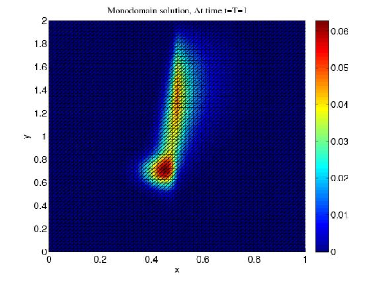
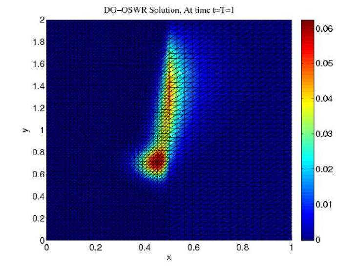
The physical domain is , the final time is . The initial value is and the right-hand side is . The domain is split into two subdomains and . The reaction is zero, the advection and diffusion coefficients are , , and , . The mesh size over the interface and time step in are and , while in , and . In Figure 2, we observe, at final time , that the approximate solution computed using 3 iterations (right figure) is close to the variational solution computed in one time window on a time conforming finergrid (left figure).
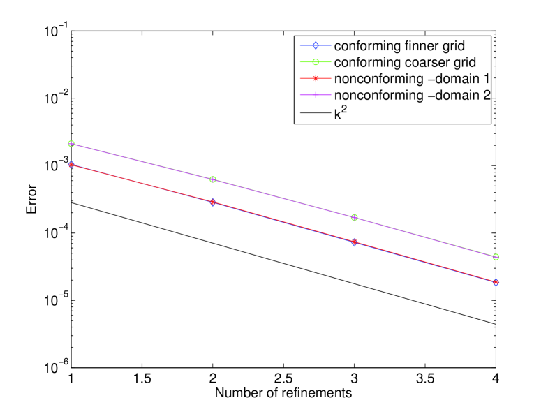
We analyze now the precision in time. The space mesh is conforming and the converged solution is such that the residual is smaller than . We compute a variational reference solution on a time grid with 4096 time steps. The nonconforming solutions are interpolated on the previous grid to compute the error. We start with a time grid with 128 time steps for the left domain and 94 time steps for the right domain. Thereafter the time step is divided by 2 several times. Figure 3 shows the norms of the error in versus the number of refinements, for both subdomains. First we observe the order in time for the nonconforming case. This fits the theoretical estimates, even though we have theoretical results only for Robin transmission conditions. Moreover, the error obtained in the nonconforming case, in the subdomain where the grid is finer, is nearly the same as the error obtained in the conforming finer case.
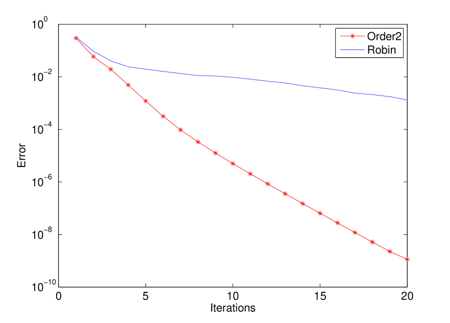
The computations are done using Order 2 transmission conditions. Indeed, the error between the multidomain and the variational solutions decrease much faster with the Order 2 transmissions conditions than with the Robin transmissions conditions as we can see in Figure 4, in the conforming case.
We now consider the advection-diffusion equation with discontinuous porosity :
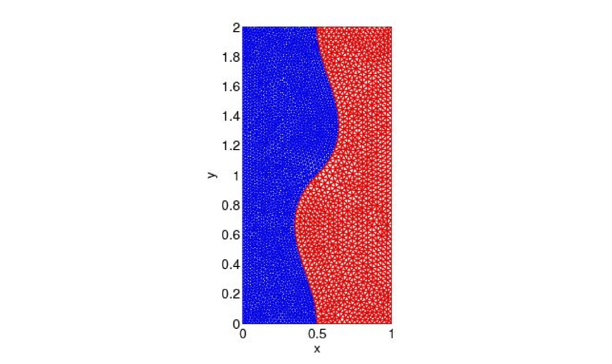
The physical domain is , the final time is . is split into two subdomains. The interface is parametrized with a Hermite polynomial , see Figure 5.
The advection, diffusion and porosity
coefficients are
, ,
,
, , .
We first consider a conforming grid in space. The time step in is , while in , . In Figure 6, we observe, at final time , the approximate solution computed using ten time windows and 5 iterations in each time window. It is close to the variational solution computed in one time window on the conforming finer space-time grid as shown on the error, in Figure 7.
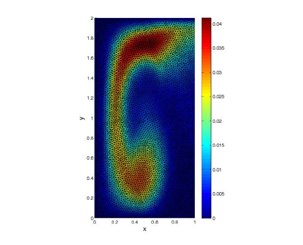 Fig. 6: DG-OSWR solution after 10 time
windows and 5 iterations per window
Fig. 6: DG-OSWR solution after 10 time
windows and 5 iterations per window
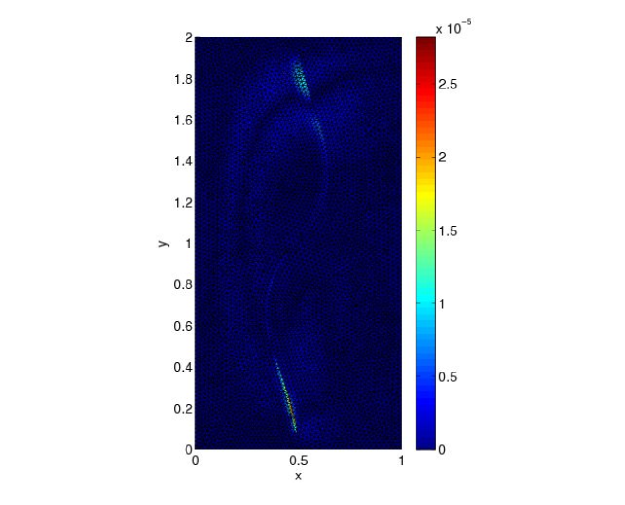 Fig. 7: Error with variational solution after 10 time
windows and 5 iterations per window
Fig. 7: Error with variational solution after 10 time
windows and 5 iterations per window
We analyze in Figure 8 the precision versus the time step. The converged solution is such that the residual is smaller than . A variational reference solution is computed on a time grid with 7680 time steps. The time nonconforming solutions are interpolated on the previous grid to compute the error. We start with a time grid with 120 time steps for the left domain and 26 time steps for the right domain and divide by 2 the time steps several times. Figure 8 shows the norms of the error in versus the time steps, for both subdomains.
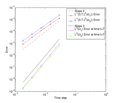
We observe the order in time for the nonconforming case that fits the theoretical estimates. In Figure 8 we show also the norms of the error in at final time versus the time steps, for both subdomains. We observe the order for the time nonconforming case. This corresponds to the superconvergence behavior described in [13].
We now consider nonconforming grids in space as well. The mesh size and time step in are and , while in , and . In Figure 9 we observe, at final time , that the approximate solution computed using 5 iterations in one time window is close to the solution computed with the conformal in space grid in Figure 6, left. In Figure 10 and 11 we observe the precision versus the mesh size. The converged solution is such that the residual is smaller than . A variational reference solution is computed on a time grid with 960 time steps and a space grid with mesh size . The space-time nonconforming solutions are interpolated on the previous grid to compute the error. We start with a time grid with 60 time steps and a mesh size for the left domain and 20 time steps a mesh size for the right domain and divide by 2 the time step and mesh size several times. Figure 10 shows the norms of the error in versus the time steps, for both subdomains. We observe the order for the nonconforming space-time case, even though we have theoretical results only for the time semi-discrete case. Figure 11 displays the norms of the error in and in at final time versus the mesh size, for both subdomains. We observe the order for the error, and the order for the error for the nonconforming space-time case.
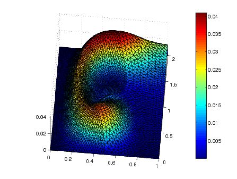
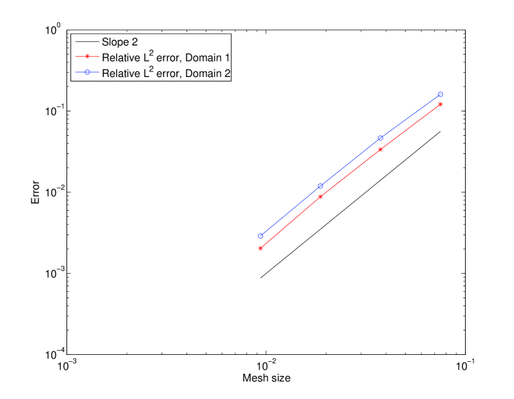 Fig. 10: Relative error in time and space
|
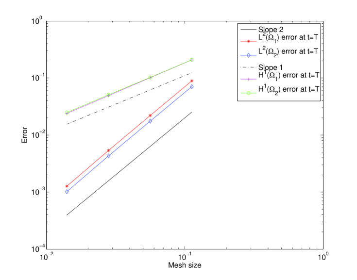 Fig. 11: and errors at the final time
|
6 Conclusion
We have proposed a new numerical method to solve parabolic equations with discontinuous coefficients. It relies on the splitting of the time interval into time windows, in which a few iterations of an optimized Schwarz waveform relaxation algorithm are performed by a discontinuous Galerkin method in time, with non conforming projection between space-time grids on the interfaces. We have shown theoretically in the Robin case that the method preserves the order of the discontinuous Galerkin method. Numerical estimates of the error and the error at final time have shown that the method preserves the order of the space nonconforming scheme as well. The analysis of the fully discrete scheme will be done in a further work.
References
- [1] D. Bennequin, M.J. Gander, and L.Halpern. A homographic best approximation problem with application to optimized Schwarz waveform relaxation. Math. Comp., 78:185–223, 2009.
- [2] E. Blayo, L. Halpern, and C. Japhet. Optimized Schwarz waveform relaxation algorithms with nonconforming time discretization for coupling convection-diffusion problems with discontinuous coefficients. In O.B. Widlund and D.E. Keyes, editors, Decomposition Methods in Science and Engineering XVI, volume 55 of Lecture Notes in Computational Science and Engineering, pages 267–274. Springer, 2007.
- [3] Philippe Charton, Frédéric Nataf, and Francois Rogier. Méthode de décomposition de domaine pour l’équation d’advection-diffusion. C. R. Acad. Sci., 313(9):623–626, 1991.
- [4] Martin J. Gander, Laurence Halpern, and Frédéric Nataf. Optimal convergence for overlapping and non-overlapping Schwarz waveform relaxation. In C-H. Lai, P. Bjørstad, M. Cross, and O. Widlund, editors, Eleventh international Conference of Domain Decomposition Methods. ddm.org, 1999.
- [5] M.J. Gander and L. Halpern. Optimized Schwarz waveform relaxation methods for advection reaction diffusion problems. SIAM Journal on Numerical Analysis, 45(2):666–697, 2007.
- [6] M.J. Gander, L. Halpern, and M. Kern. Schwarz waveform relaxation method for advection–diffusion–reaction problems with discontinuous coefficients and non-matching grids. In O.B. Widlund and D.E. Keyes, editors, Decomposition Methods in Science and Engineering XVI, volume 55 of Lecture Notes in Computational Science and Engineering, pages 916–920. Springer, 2007.
- [7] M.J. Gander, L. Halpern, and F. Nataf. Optimal Schwarz waveform relaxation for the one dimensional wave equation. SIAM Journal of Numerical Analysis, 41(5):1643–1681, 2003.
- [8] M.J. Gander, C. Japhet, Y. Maday, and F. Nataf. A New Cement to Glue Nonconforming Grids with Robin Interface Conditions : The Finite Element Case. In R. Kornhuber, R. H. W. Hoppe, J. Périaux, O. Pironneau, O. B. Widlund, and J. Xu, editors, Domain Decomposition Methods in Science and Engineering, volume 40 of Lecture Notes in Computational Science and Engineering, pages 259–266. Springer, 2005.
- [9] L. Halpern and C. Japhet. Discontinuous Galerkin and Nonconforming in Time Optimized Schwarz Waveform Relaxation for Heterogeneous Problems. In U. Langer, M. Discacciati, D.E. Keyes, O.B. Widlund, and W. Zulehner, editors, Decomposition Methods in Science and Engineering XVII, volume 60 of Lecture Notes in Computational Science and Engineering, pages 211–219. Springer, 2008.
- [10] L. Halpern, C. Japhet, and J. Szeftel. Discontinuous Galerkin and nonconforming in time optimized Schwarz waveform relaxation. In Proceedings of the Eighteenth International Conference on Domain Decomposition Methods, 2009. http://numerik.mi.fu-berlin.de/DDM/DD18/ in electronic form. To appear in printed form in the proceedings of DD19.
- [11] L. Halpern, C. Japhet, and J. Szeftel. Space-time nonconforming Optimized Schwarz Waveform Relaxation for heterogeneous problems and general geometries. In Proceedings of the Eighteenth International Conference on Domain Decomposition Methods, 2010. accepted.
- [12] Caroline Japhet. Méthode de décomposition de domaine et conditions aux limites artificielles en mécanique des fluides : méthode Optimisée d’Ordre 2 (OO2). PhD thesis, Université Paris 13, France, 1998.
- [13] Claes Johnson and Kenneth Eriksson. Adaptive finite element methods for parabolic problems ii: Optimal error estimates in and . SIAM J. Numer.Anal., 32, 1995.
- [14] Claes Johnson, Kenneth Eriksson, and Vidar Thomee. Time discretization of parabolic problems by the discontinuous Galerkin method. RAIRO Modél. Math. Anal. Numér., 19, 1985.
- [15] J-L Lions and E. Magenes. Problèmes aux limites non homogènes et applications, volume 18 of Travaux et recherches mathématiques. Dunod, 1968.
- [16] C. Makridakis and R. Nochetto. A posteriori error analysis for higher order dissipative methods for evolution problems. Numer. Math., 104, 2006.
- [17] V. Martin. An optimized Schwarz waveform relaxation method for unsteady convection diffusion equation. Appl. Numer. Math., 52(4):401–428, 2005.
- [18] Jérémie Szeftel. Absorbing boundary conditions for reaction-diffusion equations. IMA J. Appl. Math., 68(2):167–184, 2003.
- [19] Jérémie Szeftel. Calcul pseudo-différentiel et para-différentiel pour l’étude des conditions aux limites absorbantes et des propriétés qualitatives des EDP non linéaires. PhD thesis, Université Paris 13, France, 2004.
- [20] Vidar Thomee. Galerkin Finite Element Methods for Parabolic Problems. Springer, 1997.