Optimized Tradeoffs for Private Prediction with Majority Ensembling
Abstract
We study a classical problem in private prediction, the problem of computing an -differentially private majority of -differentially private algorithms for and . Standard methods such as subsampling or randomized response are widely used, but do they provide optimal privacy-utility tradeoffs? To answer this, we introduce the Data-dependent Randomized Response Majority (DaRRM) algorithm. It is parameterized by a data-dependent noise function , and enables efficient utility optimization over the class of all private algorithms, encompassing those standard methods. We show that maximizing the utility of an -private majority algorithm can be computed tractably through an optimization problem for any by a novel structural result that reduces the infinitely many privacy constraints into a polynomial set. In some settings, we show that DaRRM provably enjoys a privacy gain of a factor of 2 over common baselines, with fixed utility. Lastly, we demonstrate the strong empirical effectiveness of our first-of-its-kind privacy-constrained utility optimization for ensembling labels for private prediction from private teachers in image classification. Notably, our DaRRM framework with an optimized exhibits substantial utility gains when compared against several baselines.
1 Introduction
Differential privacy (DP) is a widely applied framework for formally reasoning about privacy leakage when releasing statistics on a sensitive database Erlingsson et al. (2014); Cormode et al. (2018). Differential privacy protects data privacy by obfuscating algorithmic output, ensuring that query responses look similar on adjacent datasets while preserving utility as much as possible Dwork et al. (2006).
Privacy in practice often requires aggregating or composing multiple private procedures that are distributed for data or training efficiency. For example, it is common to aggregate multiple private algorithmic or model outputs in methods such as boosting or calibration (Sagi & Rokach, 2018). In federated learning, model training is distributed across multiple edge devices. Those devices need to send local information, such as labels or gradients Konečnỳ et al. (2016), to an aggregating server, which is often honest but curious about the local training data. Hence, the output from each model at an edge device needs to be privatized locally before being sent to the server. When translating from a local privacy guarantee to a centralized one, one needs to reason about the composition of the local privacy leakage Naseri et al. (2020). Therefore, we formally ask the following:
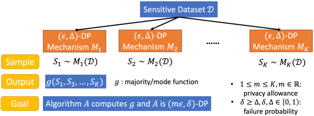
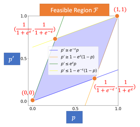
Problem 1.1 (Private Majority Ensembling (Illustrated in Figure 1)).
Consider -differentially private mechanisms for odd. Given a dataset , each mechanism outputs a binary answer — that is, , . Given a privacy allowance , and a failure probability , , how can one maximize the utility of an -differentially private mechanism to compute the majority function , where ?
The majority function is often used in private prediction, where one studies the privacy cost of releasing one prediction Dwork & Feldman (2018) and exploits the fact that releasing only the aggregated output on sharded models is significantly more private than releasing each prediction. For example, this occurs in semi-supervised knowledge transfer with private aggregated teacher ensembles (PATE) Papernot et al. (2017; 2018), in ensemble learning algorithms Jia & Qiu (2020); Xiang et al. (2018), machine unlearning Bourtoule et al. (2021), private distributed learning algorithms such as Stochastic Sign-SGD Xiang & Su (2023), and in ensemble feature selection Liu et al. (2018). Private prediction is also shown to be a competitive technique in data-adaptive settings, where the underlying dataset is changing slowly over time, to quickly adjust to online dataset updates Zhu et al. (2023). Furthermore, to address the large privacy loss of private prediction under the many-query regime, there has been recent works in everlasting private prediction that extends privacy guarantees with repeated, possibly infinite, queries without suffering a linear increase in privacy loss Naor et al. (2023); Stemmer (2024).
These works, however, rely often on the standard sensitivity analysis of to provide a private output and thus generally provide limited utility guarantees. This is because the maximum sensitivity of can be too pessimistic in practice, as observed in the problem of private hyperparameter optimization (Liu & Talwar, 2019). On the other hand, for private model ensembling, a naive way to bound privacy loss without restrictive assumptions is to apply simple composition (Theorem 2.2) or general composition (Theorem 2.3, a tighter version compared to advanced composition) to reason about the final privacy loss after aggregation. A black-box application of the simple composition theorem to compute would incur a privacy cost in the pure differential privacy setting, that is, , or if one is willing to tolerate some failure probability , general composition would yield a privacy cost Kairouz et al. (2015). Thus, a natural baseline algorithm that is -differentially private applies privacy amplification by subsampling and randomly chooses of the mechanisms to aggregate and returns the majority of the subsampled mechanisms. This technique is reminiscent of the subsampling procedure used for the maximization function (Liu & Talwar, 2019) or some general techniques for privacy amplification in the federated setting via shuffling (Erlingsson et al., 2019).
However, standard composition analysis and privacy amplication techniques can be suboptimal for computing a private majority, in terms of both utility and privacy. Observe that if there is a clear majority among the outputs of , one can add less noise. This is because each mechanism is -differentially private already, and hence, is less likely to change its output on a neighboring dataset by definition. This implies the majority outcome is unlikely to change based on single isolated changes in . Furthermore, composition theorems make two pessimistic assumptions: 1) the worst-case function and the dataset are considered, and 2) all intermediate mechanism outputs are released, rather than just the final aggregate. Based on these observations, is it possible then to improve the utility of computing a private majority, under a fixed privacy loss?
1.1 Our Contributions
We give a (perhaps surprising) affirmative answer to the above question by using our novel data-dependent randomized response framework (DaRRM), which captures all private majority algorithms, we introduce a tractable noise optimization procedure that maximizes the privacy-utility tradeoffs. Furthermore, we can provably achieve a constant factor improvement in utility over simple subsampling by applying data-dependent noise injection when ’s are i.i.d. and . To our knowledge, this is the first of its work of its kind that gives a tractable utility optimization over the possibly infinite set of privacy constraints.
Data-dependent Randomized Response Majority (DaRRM). We generalize the classical Randomized Response (RR) mechanism and the commonly used subsampling baseline for solving Problem 1.1 and propose a general randomized response framework DaRRM (see Algorithm 1), which comes with a customizable noise function . We show that DaRRM actually captures all algorithms computing the majority whose outputs are at least as good as a random guess (see Lemma 3.3), by choosing different functions.
Designing with Provable Privacy Amplification. The choice of the function in DaRRM allows us to explicitly optimize noise while trading off privacy and utility. Using structural observations, we show privacy amplification by a factor of 2 under mild conditions over applying simple composition in the pure differential privacy setting when the mechanisms ’s are i.i.d. (see Theorem 4.1).
Finding the Best through Dimension-Reduced Optimization. We further exploit the generality of DaRRM by applying a novel optimization-based approach that applies constrained optimization to find a data-dependent that maximizes some measure of utility. One challenge is that there are infinitely many privacy constraints, which are necessary for DaRRM with the optimized to satisfy the given privacy loss. We show that we can reformulate the privacy constraints, which are infinite dimensional, to a finite polynomial-sized constraint set, allowing us to efficiently constrain the optimization problem to find the best , even for approximate differential privacy (see Lemma 5.1). Empirically, we show that with a small and , the optimized (see in Figure 2) achieves the best utility among all functions, even compared to the subsampling and the data-independent baseline. To our knowledge, this is the first utility maximization algorithm that optimizes over all private algorithms by constrained optimization with dimension reduction.
Experiments. In downstream tasks, such as semi-supervised knowledge transfer for private image classification, we compare our DaRRM with an optimized to compute the private label majority from private teachers against PATE Papernot et al. (2018), which computes the private label majority from non-private teachers. We fix the privacy loss of the output of both algorithms to be the same and find that when the number of teachers is small, DaRRM indeed has a higher utility than PATE, achieving 10%-15% and 30% higher accuracy on datasets MNIST and Fashion-MNIST, respectively.
2 Background
2.1 Related Work
Private Composition. Blackbox privacy composition analysis often leads to pessimistic utility guarantees. In the blackbox composition setting, one can do no better than the privacy analysis for pure differential privacy Dwork et al. (2014). For approximate differential privacy, previous work has found optimal constants for advanced composition by reducing to the binary case of hypothesis testing with randomized response; and optimal tradeoffs between for black box composition are given in Kairouz et al. (2015), where there could be a modest improvement .
Thus, for specific applications, previous work has turned to white-box composition analysis for improved utility. This includes, for example, moment accountant for private SGD Abadi et al. (2016) and the application of contractive maps in stochastic convex optimization Feldman et al. (2018). For the specific case of model ensembles, Papernot et al. (2018) shows a data-dependent privacy bound that vanishes as the probability of disagreement goes to . Their method provides no utility analysis but they empirically observed less privacy loss when there is greater ensemble agreement.
When is the maximization function, some previous work shows that an approximately maximum value can be outputted with high probability while incurring privacy loss, independently of . Liu & Talwar (2019) proposed a random stopping mechanism for that draws samples uniformly at random from at each iteration. In any given iteration, the sampling halts with probability and the final output is computed based on the samples collected until that time. This leads to a final privacy cost of only for the maximization function , which can be improved to (Papernot & Steinke, 2022). In addition to the aforementioned works, composing top-k and exponential mechanisms also enjoy slightly improved composition analysis via a bounded-range analysis Durfee & Rogers (2019); Dong et al. (2020).
Bypassing the Global Sensitivity. To ensure differential privacy, it is usually assumed the query function has bounded global sensitivity — that is, the output of does not change much on any adjacent input datasets differing in one entry. The noise added to the output is then proportional to the global sensitivity of . If the sensitivity is large, the output utility will thus be terrible due to a large amount of noises added. However, the worst case global sensitivity can be rare in practice, and this observation has inspired a line of works on designing private algorithms with data-dependent sensitivity bound to reduce the amount of noises added.
Instead of using the maximum global sensitivity of on any dataset, the classical Propose-Test-Release framework of Dwork Dwork & Lei (2009) uses a local sensitivity value for robust queries that is tested privately and if the sensitivity value is too large, the mechanism is halted before the query release. The halting mechanism incurs some failure probability but deals with the worst-case sensitivity situations, while allowing for lower noise injection in most average-case cases.
One popular way to estimate average-case sensitivity is to use the Subsample-and-Aggregate framework by introducing the notion of perturbation stability, also known as local sensitivity of a function on a dataset Thakurta & Smith (2013); Dwork et al. (2014), which represents the minimum number of entries in needs to be changed to change . One related concept is smooth sensitivity, a measure of variability of in the neighborhood of each dataset instance. To apply the framework under smooth sensitivity, one needs to privately estimate a function’s local sensitivity and adapt noise injection to be order of , where can often be as small as , where , the total dataset size Nissim et al. (2007). Generally, the private computation of the smooth sensitivity of a blackbox function is nontrivial but is aided by the Subsample and Aggregate approach for certain functions.
These techniques hinge on the observation that a function with higher stability on requires less noise to ensure worst case privacy. Such techniques are also applied to answer multiple online functions/queries in model-agnostic learning Bassily et al. (2018). However, we highlight two key differences in our setting with a weaker stability assumption. First, in order to estimate the perturbation stability of on , one needs to downsample or split into multiple blocks Thakurta & Smith (2013); Dwork et al. (2014); Bassily et al. (2018), , and estimate the perturbation stability based on the mode of . This essentially reduces the amount of change in the output of due to a single entry in , with high probability and replaces the hard-to-estimate perturbation stability of with an easy-to-compute perturbation stability of the mode. Such a notion of stability has also been successfully applied, along with the sparse vector technique, for model-agnostic private learning to handle exponentially number of queries to a model Bassily et al. (2018). Note that in these cases, since a private stochastic test is applied, one cannot achieve pure differential privacy Dwork et al. (2014). In practice, e.g. federated learning, however, one does not have direct access to , and thus it is impractical to draw samples from or to split . Second, to ensure good utility, one relies on a key assumption, i.e. the subsampling stability of , which requires with high probability over the draw of subsamples .
Although our intuition in designing DaRRM also relies on the stability of the mode function , previous usage of stability to improve privacy-utility tradeoffs, e.g., propose-test-release Vadhan (2017); Dwork et al. (2014), requires the testing of such stability, based on which one adds a larger (constant) noise . This can still lead to adding redundant noise in our case.
Optimal Randomized Response. Holohan et al. (2017) and Kairouz et al. (2015) show that the classical Randomized Response (RR) mechanism with a constant probability of faithfully revealing the true answer is optimal in certain private estimation problems. Our proposed DaRRM framework and our problem setting is a generalized version of the ones considered in both Holohan et al. (2017) and Kairouz et al. (2015), which not only subsumes RR but also enables a data-dependent probability, or noise addition.
While RR with a constant probability can be shown optimal in problems such as private count queries or private estimation of trait possession in a population, it is not optimal in other problems, such as private majority ensembling, since unlike the former problems, changing one response of the underlying mechanisms does not necessarily change the output of the majority. To explicitly compute the minimum amout of noise required, one needs the output distributions of the underlying mechanisms but this is unknown. To resolve this, our proposed DaRRM framework adds the amount of noise dependent on the set of observed outcomes from the underlying private mechanisms, , which is a random variable of the dataset and is hence a proxy. This enables DaRRM to calibrate the amount of noise based on whether the majority output is likely to change. The amount of noise is automatically reduced when the majority output is not likely to change.
Second, Holohan et al. (2017) and Kairouz et al. (2015) both consider a special case in our setting where all private mechanisms are i.i.d., while our approach focuses on the more general setting where each private mechanism can have a different output distribution.
Learning A Good Noise Distribution. There have been limited works that attempt to derive or learn a good noise distribution that improves the utility. For deep neural networks inference, Mireshghallah et al. (2020) attempts to learn the best noise distribution to maximizing utility subject to an entropy Lagrangian, but no formal privacy guarantees were derived. For queries with bounded sensitivity, Geng & Viswanath (2015) demonstrate that the optimal noise distribution is in fact a staircase distribution that approaches the Laplacian distribution as .
Private Prediction. Instead of releasing a privately trained model as in private learning, private prediction hides the models and only releases private outputs. Private prediction has been shown as a practical alternative compared to private learning, as performing private prediction is much easier compared to private learning on a wide range of tasks Dwork & Feldman (2018); Naor et al. (2023); van der Maaten & Hannun (2020). Although a privately trained model can make infinitely many predictions at the inference time without incurring additional privacy loss, since differential privacy is closed under post-processing, it has been shown recently that it is indeed possible to make infinitely many private predictions Naor et al. (2023) with a finite privacy loss for specific problems.
2.2 Preliminaries
We first introduce the definition of differential privacy, simple composition and general composition as follows. The general composition Kairouz et al. (2015) gives a near optimal and closed-form bound on privacy loss under adaptive composition, which improves upon advanced composition Dwork et al. (2014).
Definition 2.1 (Differential Privacy (DP) Dwork et al. (2014)).
A randomized mechanism with a domain and range satisfies -differential privacy for if for any two adjacent datasets and for any subset of outputs it holds that . is often called pure differential privacy; while is often called approximate differential privacy.
Theorem 2.2 (Simple Composition Dwork et al. (2014)).
For any and , the class of -differentially private mechanisms satisfy -differential privacy under -fold adaptive composition.
Theorem 2.3 (General Composition (Theorem 3.4 of Kairouz et al. (2015))).
For any and , the class of -differentially private mechanisms satisfies -differential privacy under -fold adaptive composition for
We then formalize the error and utility metric in our problem as follows:
Definition 2.4 (Error Metric and Utility Metric).
For the problem setting in Definition 1.1, let the observed (random) outcomes set be , where . For a fixed , we define the error of an algorithm , i.e., , in computing the majority function as the Total Variation (TV) distance between and . Specifically,
and the utility is defined as .
Notation. Throughout the paper, we use the same notations defined in Problem 1.1 and Definition 2.4. Furthermore, let and to denote a pair of adjacent datasets with one entry being different. Also, let and , . We omit the subscript when all ’s or ’s are equal. denotes the indicator function and . For the purpose of analysis, let , i.e. the (random) sum of all observed outcomes on dataset . is omitted when the context is clear. Unless specified, we use the noise function as input to our algorithms to calibrate the probabilistic noise injection. Unless specified, the privacy allowance .
3 Private Majority Algorithms
The very first approach to consider when solving private majority ensembling (Problem 1.1), since the output is binary, is the classical Randomized Response (RR) mechanism Dwork et al. (2014), where one flips a biased coin with a constant probability . If the coin lands on head with probability , output the true majority base on samples; if not, then simply output a noisy random answer. However, to make the output -differential private, the success probability can be at most (or ) when (or ) (see Appendix A.1), which is too small for any reasonable utility.
The key observation for improved utility is that the probability of success should not be a constant, but should depend on the unpublished set of observed outcomes from the mechanisms . If we see many 1’s or 0’s in , then there should be a clear majority even on adjacent datasets. On the other hand, if we see about half 1’s and half 0’s, this means the majority is highly volatile to data changes, which implies we need more noise to ensure privacy. In summary, if we can calibrate the success probability based on to smoothly increase when there is a clear majority, we can improve the utility without affecting privacy.
Subsampling. One natural baseline is outputting the majority of out of randomly subsampled mechanisms (without replacement), given a privacy allowance . Suppose , the privacy loss of the aggregated output can be reasoned through simple composition or general composition. Interestingly, we show outputting the majority of out of subsampled mechanisms corresponds to RR with a non-constant probability , which is set by a polynomial function based on the sum of observed outcomes in Lemma 3.1 (see a full proof in Appendix A.2). Intuitively, subsampling may be seen as implicitly adding noise by only outputting based on a randomly chosen subset of the mechanisms; therefore this implicit noise is inherently data-dependent on .
Lemma 3.1.
Consider Problem 1.1, with the privacy allowance . Consider the data-dependent algorithm that computes and then applies RR with probability . If , where is the value of , i.e., the (random) sum of observed outcomes on dataset , and is
then the majority of out of subsampled mechanisms without replacement and the output of our data-dependent RR algorithm have the same distribution.
One thing special about subsampling is that when , it indeed results in the optimal error, which we show in Lemma 3.2 as follows. See a full proof in Appendix A.3. Note that when , subsampling outputs a majority of 1 with probability exactly . This lower bound only applies to the case when , since when , the probability of subsampling outputting a majority of 1 is not necessary .
Lemma 3.2 (Lower Bound on Error when ).
Let be an -differentially private algorithm, where and , that computes the majority of -differentially private mechanisms , where on dataset and . Then, the error , where is the probability of the true majority output being 1 as defined in Definition 1.1.
Data-dependent Randomized Response (DaRRM). Does subsampling give optimal utility when ? Inspired by the connection between RR and subsampling, we propose Data-dependent Randomized Response Majority (DaRRM) in Algorithm 1, to study optimizing privacy-utility tradeoffs in private majority ensembling. In particular, DaRRM has a non-constant success probability that is set by a parameterized noise function , which in turn depends on the set of observed outcomes . In fact, we can show that DaRRM is general: any reasonable algorithm , name one whose output is at least as good as a random guess, can be captured by the DaRRM framework in Lemma 3.3 (see a full proof in Appendix A.4). We denote DaRRM instantiated with a specific noise function by .
Lemma 3.3 (Generality of DaRRM).
Let be any randomized algorithm to compute the majority function on such that for all , (i.e. is at least as good as a random guess). Then, there exists a a general function such that if one sets by in DaRRM, the output distribution of is the same as the output distribution of .
Designing the Function. With the DaRRM framework, we ask: how to design a good function that maximizes the utility? First, we introduce two characteristics of that do not affect the utility, while simplifying the analysis and the empirical optimization:
-
(a)
A function of the sum of observed samples: Since the observed samples set is a permutation-invariant set, a sufficient statistic that captures the full state of is , the sum of observed outcomes. This allows us to reduce . Hence, in the rest of the paper, we focus on .
-
(b)
Symmetric around : If is asymmetric, we can symmetrize by reflecting one region about and achieve better or equal expected utility, where the utility is summed over symmetric distributions of .
Note that satisfies both characteristics. Now, recall and are the sum of observed outcomes on adjacent datasets and . Also, recall and are the output probabilities of the mechanism on . To design a good noise function in DaRRM, we start by deriving conditions for a function such that is -differentially private in Lemma 3.4 (see a full proof in Appendix A.5).
4 Provable Privacy Amplification
We theoretically demonstrate that privacy is provably amplified under improved design of in our DaRRM framework. Specifically, we show when the mechanisms are i.i.d. and , we gain privacy amplification by a factor of 2 compared to the naïve subsampling baseline by carefully designing .
Theorem 4.1 (Provable Privacy Amplification by 2).
Interpretation. First, when is small, the in Theorem 4.1 corresponds to outputting the majority based on subsampling outcomes, from Lemma 3.1. However, the subsampling baseline, whose privacy loss is reasoned through simple composition, would have indicated that one can only output the majority based on outcomes, therefore implying a x privacy gain. When , the above theorem indicates that we can set a constant , which implies we are optimally outputting the true majority with no noise while still surprisingly ensuring privacy.
Intuition. This x privacy gain is intuitively possible because the majority is only dependent on half of the mechanisms’ outputs, therefore the privacy leakage is also halved. To see this, we start by analyzing the privacy cost objective in Eq. 31, where with a careful analysis of its gradient, we show that the maximum indeed occurs when satisfies certain conditions. Now, when , note that the probability ratio of outputting with outcomes is approximately , where dependence on follows because the probability of outputting is dominated by the probability that exactly mechanisms output 1. To rigorize this, we derive sufficient conditions for functions that satisfy as indicated by Lemma 3.4, to ensure DaRRM to be -differentially private and a more detailed overview and the full proof can be found in Appendix B.
5 Optimizing the Noise Function in DaRRM
Theoretically designing and extending privacy amplification results to the case is difficult and it is likely that our crafted is far from optimal. On the other hand, one can optimize for such that maximizes the utility but this involves solving a “Semi-infinite Programming” problem, due to the infinitely many privacy constraints, which are the constraints in the optimization problem necessary to ensure DaRRM with the optimized satisfy a given privacy loss. Solving a “Semi-infinite Programming” problem in general is non-tractable, but we show that in our specific setting this is in fact tractable, proposing a novel learning approach based on DaRRM that can optimize the noise function to maximize the utility. To the best of our knowledge, such optimization, presented as follows, is the first of its kind:
| (2) | ||||
| (3) | ||||
where is the privacy cost objective as defined in Lemma 3.4, is the feasible region where lies due to each mechanism being -differentially private. Observe that since is symmetric around , we only need to optimize variables instead of variables. is the distribution from which are drawn. We want to stress that no prior knowledge about the dataset or the amount of consensus among the private mechanisms is required to use our optimization framework. When there is no prior knowledge about , is set to be the uniform distribution for maximizing the expected utility. Note the above optimization problem also enables the flexibility of incorporating prior knowledge about the mechanisms by choosing a prior distribution to further improve the utility.
Optimizing Over All Algorithms. We want to stress that by solving the above optimization problem, we are indeed optimizing over all algorithms for maximal utility, since we show in Lemma 3.3 DaRRM that captures all reasonable algorithms computing a private majority.
Linear Optimization Objective. Perhaps surprisingly, it turns out that optimizing for is a Linear Programming (LP) problem! Indeed, after expanding the optimization objective in Eq. 2 by the utility definition (see Definition 2.4), optimizing the above objective is essentially same as optimizing:
where and observe . The above objective is linear in . See a full derivation in Appendix C.1.
Although taking the expectation over involves integrating over variables and this can be computationally expensive, we discuss how to formulate a computationally efficient approximation of the objective in Appendix C.2, which we later use in the experiments. Note that the objective only for maximizing the utility and hence approximating the objective does not affect the privacy guarantee.
Reducing Infinitely Many Constraints to A Polynomial Set. The constraints in the optimization problem (Eq. 3) is what makes sure the output of is -differentially private. We thus call them the privacy constraints. Note that the privacy constraints are linear in .
Though it appears we need to solve for infinitely many such privacy constraints since ’s and ’s are continuous, we show that through a structural understanding of DaRRM, we can reduce the number of privacy constraints from infinitely many to exponentially many, and further to a polynomial set. First, we observe the privacy cost objective is linear in each independent pair of fixing all , , and hence finding the worst case probabilities in given any , is a linear programming (LP) problem. Furthermore, since and are the probability of outputting 1 from the -th -differentially private mechanism on adjacent datasets, by definition, they are close and lie in a feasible region , which we show has 8 corners if (and only 4 corners if ). This implies only happens at one of the corners of , and hence the number of constraints reduces to (and if ). Second, observe that and in the privacy cost objective are the pmf of two Poisson Binomial distributions at . Notice that the Poisson Binomial is invariant under the permutation of its parameters, i.e. has the same distribution as , under some permutation . Based on this observation, we show the number of constraints can be further reduced to if (and if ). We formalize the two-step reduction of the number of privacy constraints in Lemma 5.1 as follows. See a full proof in Appendix C.3. 111Practical Limitation. Although the number of constraints is polynomial in and optimizing in DaRRM is an LP, can still make the number of constraints intractably large when is large. In practice, we observe with the Gurobi optimizer, one can optimize for on a laptop if . But if , since the number of privacy constraints is , one can optimize for over 100.
Lemma 5.1.
Consider using DaRRM (Algorithm 1) to solve Problem 1.1 and let be the privacy cost objective as defined in Lemma 3.4. Given an arbitrary noise function , let the worst case probabilities be .
Then, each pair satisfies
Furthermore, when , there exists a finite vector set of size such that if , then . When , the size of can be reduced to .
6 Experiments
We empirically solve222All code for the experiments can be found at https://anonymous.4open.science/r/OptimizedPrivateMajority-CF50 the above optimization problem (Eq. 2) using the Gurobi333https://www.gurobi.com/ solver and first present the shape of the optimized function, which we call , and its utility in Section 6.1. Then, we demonstrate the compelling effectiveness of DaRRM with an optimized function, i.e., , in ensembling labels for private prediction from private teachers through the application of semi-supervised knowledge transfer for private image classification in Section 6.2.
6.1 Optimized in Simulations
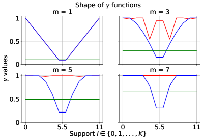
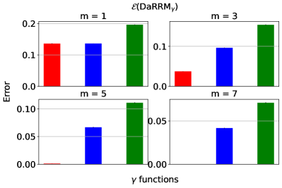

, and the baselines (corresponding to subsampling) and (corresponding to RR). Here, , , and .
We compare the shape and the error of different functions: an optimized and the subsampling as in Lemma 3.1444Note the subsampling mechanism from Section 4, which enjoys a privacy amplification by a factor of 2, only applies to pure differential privacy settings (i.e., when ). However, we focus on the more general approximate differential privacy settings (with ) in the experiments, and hence, the subsampling baseline we consider throughout this section is the basic version without privacy amplification. To see how the subsampling mechanism from Section 4 with privacy amplification compares against the other algorithms, please refer to Appendix D.1.2.. We also compare against in the classical baseline RR (see Section A.1) and . Here, can be viewed as a constant noise function ; and is the same as .
We present the results with and . We assume there is no prior knowledge about the mechanisms , and set the prior distribution from which ’s are drawn, , to be the uniform distribution, in the optimization objective (Eq. 2) searching for . To ensure a fair comparison against the subsampling baseline, we set to be the one by -fold general composition (see Theorem 2.3), which in this case, is . We plot each functions over the support and the corresponding error of each algorithm in Figure 2.
Discussion. In summary, at , the optimized noise function overlaps with which corresponds to the subsampling baseline. This agrees with our lower bound on the error in Lemma 3.2, which implies that at , subsampling indeed gives the optimal error. When , the optimized noise function has the highest probability of outputting the true majority over the support than the functions corresponding to the baselines. This implies has the lowest error (and hence, highest utility), which is verified on the bottom set of plots. More results on comparing the optimized under the uniform against the baselines by general composition (Theorem 2.3) and in pure differential privacy settings (i.e., ) for large and can be found in Appendix D.1.1 and D.1.2. Furthermore, we include results optimizing using a non-uniform prior in Appendix D.1.3.
6.2 Private Semi-Supervised Knowledge Transfer
Dataset MNIST # Queries GNMax (Baseline) (Baseline) (Ours) 0.63 (0.09) 0.76 (0.09) 0.79 (0.09) 0.66 (0.06) 0.75 (0.06) 0.79 (0.05) 0.64 (0.04) 0.76 (0.04) 0.80 (0.04)
Dataset Fashion-MNIST # Queries GNMax (Baseline) (Baseline) (Ours) 0.65 (0.11) 0.90 (0.07) 0.96 (0.03) 0.59 (0.06) 0.94 (0.03) 0.96 (0.02) 0.64 (0.04) 0.93 (0.02) 0.96 (0.02)
-differentially private. With the same per query privacy loss (and hence the same total privacy loss over samples), achieves the highest accuracy compared to the other two baselines.
Semi-supervised Knowledge Transfer. We apply our DaRRM framework in the application of semi-supervised knowledge transfer for private image classification. We follow a similar setup as in PATE Papernot et al. (2017; 2018), where one trains teachers, each on a subset of a sensitive dataset, and at the inference time, queries the teachers for the majority of their votes, i.e., the predicted labels, of a test sample. Each time the teachers are queried, there is a privacy loss, and we focus on this private prediction subroutine in this section. To limit the total privacy loss over all queries, the student model is also trained on a public dataset without labels. The student model queries the labels of a small portion of the samples in this dataset from the teachers and is then trained using semi-supervised learning algorithms on both the labeled and unlabeled samples from the public dataset.
Baselines. We want the privacy loss per query of a test sample to the teachers to be . This can be achieved via two ways: 1) Train non-private teachers, add Gaussian noise to the number of predicted labels from the teachers in each output class, and output the majority of the noisy votes. This is exactly the GNMax algorithm from PATE Papernot et al. (2018). 2) Train -differentially private teachers and output the majority of the teachers’ votes by adding a smaller amount of noise. This can be computed using DaRRM with an appropriate noise function . We compare the performance of GNMax and DaRRM with two functions: (i.e., the optimized ), and (i.e., the subsampling baseline). The overall privacy loss over queries to the teachers can be computed by general composition (Theorem 2.3).
Experiment Setup. We use samples from two randomly chosen classes — class 5 and 8 — from the MNIST and Fashion-MNIST datasets to form our training and testing datasets. Our MNIST has a total of 11272 training samples and testing samples; our Fashion-MNIST has training samples and testing samples. We train teachers on equally divided subsets of the training datasets. Each teacher is a CNN model. The non-private and private teachers are trained using SGD and DP-SGD Abadi et al. (2016), respectively, for 5 epochs. DaRRM Setup: The Gaussian noise in DP-SGD has zero mean and std. ; the gradient norm clipping threshold is . This results in each private teacher, trained on MNIST and Fashion-MNIST, being and -differentially private, respectively, after 5 epochs. We set the privacy allowance 555 Here, we present results with privacy allowance because we think this is a more interesting case. is less interesting, since one cannot get improvement compared to the subsampling baseline. close to a is also less interesting, as this case seems too easy for our proposed method (the optimized function is very close to 1, meaning very little noise needs to be added in this case). Hence, we pick , which is a case when improvement is possible, and is also potentially challenging for our optimization framework. This is also realistic as most applications would only want to tolerate a constant privacy overhead. See more results with different privacy allowance ’s in this setting in Appendix D.2.2. and the privacy loss per query is then computed using general composition under -fold, which give the same privacy loss in the high privacy regime, resulting in on MNIST and on Fashion-MNIST. GNMax Setup: We now compute the std. of the Gaussian noise used by GNMax to achieve a per-query privacy loss of , as in the DaRRM setup. We optimize according to the Renyi differential privacy loss bound of Gaussian noise. Although Papernot et al. (2018) gives a potentially tighter data-dependent privacy loss bound for majority ensembling non-private teachers, we found when and the number of output classes are small as in our case, even if all teachers agree on a single output class, the condition of the data-dependent bound is not satisfied. Hence, we only use the privacy loss bound of Gaussian noise here to set in GNMax. See Appendix D.2.1 for more details, including the values and other parameters. Finally, the per sample privacy loss and the total privacy loss over queries, which is computed by advanced composition, are reported in Table 9.
The testing dataset is treated as the public dataset on which one trains a student model. Papernot et al. (2018) empirically shows querying samples from a public dataset of size suffices to train a student model with a good performance. Therefore, we pick . We repeat the selection of samples 10 times and report the mean test accuracy with one std. in parentheses in Table 1. The queries serve as the labeled samples in training the student model. The higher the accuracy of the labels from the queries, the better the final performance of the student model. We skip the actual training of the student model using semi-supervised learning algorithms here.
| Dataset | # Queries | Privacy loss per query | Total privacy loss over queries |
|---|---|---|---|
| MNIST | |||
| Fashion MNIST | |||
Discussion. Table 1 shows achieves the highest accuracy (i.e., utility) compared to the two baselines on both datasets. First, comparing to , we verify that subsampling does not achieve a tight privacy-utility tradeoff, and we can optimize the noise function in DaRRM to maximize the utility given a target privacy loss. Second, comparing to GNMax, the result shows there are regimes where ensembling private teachers gives a higher utility than directly ensembling non-private teachers, assuming the outputs in both settings have the same privacy loss. Intuitively, this is because ensembling private teachers adds fine-grained noise during both training the teachers and aggregation of teachers’ votes, while ensembling non-private teachers adds a coarser amount of noise only to the teachers’ outputs. This further motivates private prediction from private teachers and the practical usage of DaRRM, in addition to the need of aggregating private teachers in federated learning settings with an honest-but-curious server.
7 Conclusion
In computing a private majority from private mechanisms, we propose the DaRRM framework, which is provably general, with a customizable function. We show a privacy amplification by a factor of 2 in the i.i.d. mechanisms and a pure differential privacy setting. For the general setting, we propose an tractable optimization algorithm that maximizes utility while ensuring privacy guarantees. Furthermore, we demonstrate the empirical effectiveness of DaRRM with an optimized . We hope that this work inspires more research on the intersection of privacy frameworks and optimization.
References
- Abadi et al. (2016) Martin Abadi, Andy Chu, Ian Goodfellow, H Brendan McMahan, Ilya Mironov, Kunal Talwar, and Li Zhang. Deep learning with differential privacy. In Proceedings of the 2016 ACM SIGSAC conference on computer and communications security, pp. 308–318, 2016.
- Bassily et al. (2018) Raef Bassily, Om Thakkar, and Abhradeep Thakurta. Model-agnostic private learning via stability. arXiv preprint arXiv:1803.05101, 2018.
- Bourtoule et al. (2021) Lucas Bourtoule, Varun Chandrasekaran, Christopher A Choquette-Choo, Hengrui Jia, Adelin Travers, Baiwu Zhang, David Lie, and Nicolas Papernot. Machine unlearning. In 2021 IEEE Symposium on Security and Privacy (SP), pp. 141–159. IEEE, 2021.
- Cormode et al. (2018) Graham Cormode, Somesh Jha, Tejas Kulkarni, Ninghui Li, Divesh Srivastava, and Tianhao Wang. Privacy at scale: Local differential privacy in practice. In Proceedings of the 2018 International Conference on Management of Data, pp. 1655–1658, 2018.
- Dong et al. (2020) Jinshuo Dong, David Durfee, and Ryan Rogers. Optimal differential privacy composition for exponential mechanisms. In International Conference on Machine Learning, pp. 2597–2606. PMLR, 2020.
- Durfee & Rogers (2019) David Durfee and Ryan M Rogers. Practical differentially private top-k selection with pay-what-you-get composition. Advances in Neural Information Processing Systems, 32, 2019.
- Dwork & Feldman (2018) Cynthia Dwork and Vitaly Feldman. Privacy-preserving prediction. In Conference On Learning Theory, pp. 1693–1702. PMLR, 2018.
- Dwork & Lei (2009) Cynthia Dwork and Jing Lei. Differential privacy and robust statistics. In Proceedings of the forty-first annual ACM symposium on Theory of computing, pp. 371–380, 2009.
- Dwork et al. (2006) Cynthia Dwork, Frank McSherry, Kobbi Nissim, and Adam Smith. Calibrating noise to sensitivity in private data analysis. In Theory of cryptography conference, pp. 265–284. Springer, 2006.
- Dwork et al. (2014) Cynthia Dwork, Aaron Roth, et al. The algorithmic foundations of differential privacy. Found. Trends Theor. Comput. Sci., 9(3-4):211–407, 2014.
- Erlingsson et al. (2014) Úlfar Erlingsson, Vasyl Pihur, and Aleksandra Korolova. Rappor: Randomized aggregatable privacy-preserving ordinal response. In Proceedings of the 2014 ACM SIGSAC Conference on Computer and Communications Security, CCS ’14, pp. 1054–1067, New York, NY, USA, 2014. Association for Computing Machinery. ISBN 9781450329576. doi: 10.1145/2660267.2660348. URL https://doi.org/10.1145/2660267.2660348.
- Erlingsson et al. (2019) Úlfar Erlingsson, Vitaly Feldman, Ilya Mironov, Ananth Raghunathan, Kunal Talwar, and Abhradeep Thakurta. Amplification by shuffling: From local to central differential privacy via anonymity. In Proceedings of the Thirtieth Annual ACM-SIAM Symposium on Discrete Algorithms, pp. 2468–2479. SIAM, 2019.
- Feldman et al. (2018) Vitaly Feldman, Ilya Mironov, Kunal Talwar, and Abhradeep Thakurta. Privacy amplification by iteration. In 2018 IEEE 59th Annual Symposium on Foundations of Computer Science (FOCS), pp. 521–532. IEEE, 2018.
- Geng & Viswanath (2015) Quan Geng and Pramod Viswanath. The optimal noise-adding mechanism in differential privacy. IEEE Transactions on Information Theory, 62(2):925–951, 2015.
- Holohan et al. (2017) Naoise Holohan, Douglas J. Leith, and Oliver Mason. Optimal differentially private mechanisms for randomised response. IEEE Transactions on Information Forensics and Security, 12(11):2726–2735, November 2017. ISSN 1556-6021. doi: 10.1109/tifs.2017.2718487. URL http://dx.doi.org/10.1109/TIFS.2017.2718487.
- Jia & Qiu (2020) Junjie Jia and Wanyong Qiu. Research on an ensemble classification algorithm based on differential privacy. IEEE Access, 8:93499–93513, 2020. doi: 10.1109/ACCESS.2020.2995058.
- Kairouz et al. (2015) Peter Kairouz, Sewoong Oh, and Pramod Viswanath. The composition theorem for differential privacy. In International conference on machine learning, pp. 1376–1385. PMLR, 2015.
- Konečnỳ et al. (2016) Jakub Konečnỳ, H Brendan McMahan, Felix X Yu, Peter Richtárik, Ananda Theertha Suresh, and Dave Bacon. Federated learning: Strategies for improving communication efficiency. arXiv preprint arXiv:1610.05492, 2016.
- Liu & Talwar (2019) Jingcheng Liu and Kunal Talwar. Private selection from private candidates. In Proceedings of the 51st Annual ACM SIGACT Symposium on Theory of Computing, STOC 2019, pp. 298–309, New York, NY, USA, 2019. Association for Computing Machinery. ISBN 9781450367059. doi: 10.1145/3313276.3316377. URL https://doi.org/10.1145/3313276.3316377.
- Liu et al. (2018) Zhongfeng Liu, Yun Li, and Wei Ji. Differential private ensemble feature selection. In 2018 International Joint Conference on Neural Networks (IJCNN), pp. 1–6, 2018. doi: 10.1109/IJCNN.2018.8489308.
- Mireshghallah et al. (2020) Fatemehsadat Mireshghallah, Mohammadkazem Taram, Prakash Ramrakhyani, Ali Jalali, Dean Tullsen, and Hadi Esmaeilzadeh. Shredder: Learning noise distributions to protect inference privacy. In Proceedings of the Twenty-Fifth International Conference on Architectural Support for Programming Languages and Operating Systems, pp. 3–18, 2020.
- Naor et al. (2023) Moni Naor, Kobbi Nissim, Uri Stemmer, and Chao Yan. Private everlasting prediction. arXiv preprint arXiv:2305.09579, 2023.
- Naseri et al. (2020) Mohammad Naseri, Jamie Hayes, and Emiliano De Cristofaro. Local and central differential privacy for robustness and privacy in federated learning. arXiv preprint arXiv:2009.03561, 2020.
- Nissim et al. (2007) Kobbi Nissim, Sofya Raskhodnikova, and Adam Smith. Smooth sensitivity and sampling in private data analysis. In Proceedings of the thirty-ninth annual ACM symposium on Theory of computing, pp. 75–84, 2007.
- Papernot & Steinke (2022) Nicolas Papernot and Thomas Steinke. Hyperparameter tuning with renyi differential privacy. In International Conference on Learning Representations, 2022. URL https://openreview.net/forum?id=-70L8lpp9DF.
- Papernot et al. (2017) Nicolas Papernot, Martin Abadi, Ulfar Erlingsson, Ian Goodfellow, and Kunal Talwar. Semi-supervised knowledge transfer for deep learning from private training data. In Proceedings of the International Conference on Learning Representations, 2017. URL https://arxiv.org/abs/1610.05755.
- Papernot et al. (2018) Nicolas Papernot, Shuang Song, Ilya Mironov, Ananth Raghunathan, Kunal Talwar, and Úlfar Erlingsson. Scalable private learning with pate. arXiv preprint arXiv:1802.08908, 2018.
- Sagi & Rokach (2018) Omer Sagi and Lior Rokach. Ensemble learning: A survey. Wiley Interdisciplinary Reviews: Data Mining and Knowledge Discovery, 8(4):e1249, 2018.
- Stemmer (2024) Uri Stemmer. Private truly-everlasting robust-prediction. arXiv preprint arXiv:2401.04311, 2024.
- Thakurta & Smith (2013) Abhradeep Guha Thakurta and Adam Smith. Differentially private feature selection via stability arguments, and the robustness of the lasso. In Conference on Learning Theory, pp. 819–850. PMLR, 2013.
- Vadhan (2017) Salil Vadhan. The Complexity of Differential Privacy, pp. 347–450. Springer International Publishing, Cham, 2017. doi: 10.1007/978-3-319-57048-8_7. URL https://doi.org/10.1007/978-3-319-57048-8_7.
- van der Maaten & Hannun (2020) Laurens van der Maaten and Awni Hannun. The trade-offs of private prediction, 2020.
- Xiang & Su (2023) Ming Xiang and Lili Su. $\beta$-stochastic sign SGD: A byzantine resilient and differentially private gradient compressor for federated learning, 2023. URL https://openreview.net/forum?id=oVPqFCI1g7q.
- Xiang et al. (2018) Tao Xiang, Yang Li, Xiaoguo Li, Shigang Zhong, and Shui Yu. Collaborative ensemble learning under differential privacy. Web Intelligence, 16:73–87, 03 2018. doi: 10.3233/WEB-180374.
- Zhang et al. (2019) Ying-Ying Zhang, Teng-Zhong Rong, and Man-Man Li. Expectation identity for the binomial distribution and its application in the calculations of high-order binomial moments. Communications in Statistics - Theory and Methods, 48(22):5467–5476, 2019. doi: 10.1080/03610926.2018.1435818. URL https://doi.org/10.1080/03610926.2018.1435818.
- Zhu et al. (2023) Yuqing Zhu, Xuandong Zhao, Chuan Guo, and Yu-Xiang Wang. " private prediction strikes back!”private kernelized nearest neighbors with individual renyi filter. arXiv preprint arXiv:2306.07381, 2023.
Appendix A Details of Section 3
A.1 Randomized Response with Constant Probability
We show the magnitude of in RR (Algorithm 2) to solve Problem 1.1, such that the output is -DP, in Lemma A.1.
Lemma A.1.
Proof of Lemma A.1.
Let denote the output of RR. Let and , where , and , are adjacent datasets. Recall each mechanism is -differentially private, and the majority of the outputs of is -differentially private. When , using simple composition, and . When , using general composition and . By definition of differential privacy (Definition 2.1), all of the following four constraints on apply:
To ensure RR is -differentially private, needs to be such that for all possible ,
| (5) | ||||
| (6) | ||||
| (7) |
Let . The above inequality of (Eq. 7) needs to hold for worst case output probabilities that cause the maximum privacy loss. That is, needs to satisfy
| (8) |
To find the worst case output probabilities, we solve the following Linear Programming (LP) problem:
| Objective: | (9) | ||||
| Subject to: | (10) | ||||
| (11) | |||||
| (12) | |||||
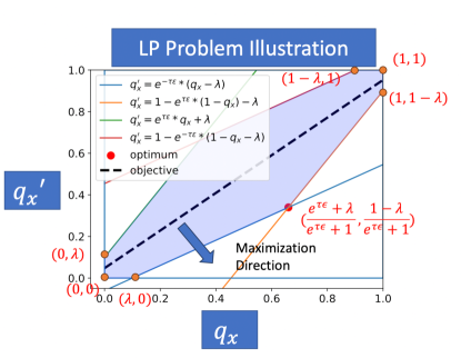
The optimum of any LP problem is at the corners of the feasible region, which is bounded by the optimization constraints. We plot the feasible region and the objective of the above LP problem in Figure 3. Here, . The optimum of the LP problem – that is, the worse case probabilities – is,
| (13) |
By Eq. 8,
| (14) | ||||
| (15) | ||||
| (16) |
For small , using the approximation and that ,
| (17) |
In the pure differential privacy setting, , and so ; and in the approximate differential privacy setting, , and so . ∎
A.2 Proof of Lemma 3.1
Lemma A.2 (Restatement of Lemma 3.1).
Consider Problem 1.1, with the privacy allowance . Consider the data-dependent algorithm that computes and then applies RR with probability . If , where is the value of , i.e., the (random) sum of observed outcomes on dataset , and is
then the majority of out of subsampled mechanisms without replacement and the output of our data-dependent RR algorithm have the same distribution.
Proof of Lemma 3.1.
Let be the sum of observed outcomes from mechanisms. Following Algorithm 3, denotes the indices chosen uniformly at random from without replacement. Conditioned on , notice the output of SubMaj follows a hypergeometric distribution. The output probability of SubMaj is
| (18) | ||||
| (19) | ||||
| (20) |
Consider an arbitrary noise function . Let denote the output of the data-dependent RR-d on dataset , where RR-d has the non-constant probability set by . The output probability of RR is,
| (21) | ||||
| (22) |
We want .
If is odd, for any , this is
| (23) |
and for any , this is
| (24) |
Similarly, if is even, for any , this is
| (25) |
and for any , this is
| (26) |
Next, we show the above is indeed symmetric around . For any , there is . If is odd,
| (27) |
Similarly, if is even,
| (28) |
makes RR-d have the same output distribution as SubMaj.
Similarly, combining Eq. 25, Eq. 26 and Eq. 28, if is even, setting as
| (30) |
makes RR-d have the same output distribution as SubMaj.
∎
A.3 Proof of Lemma 3.2
Lemma A.3 (Restatement of Lemma 3.2).
Let be an -differentially private algorithm, where and , that computes the majority of -differentially private mechanisms , where on dataset and . Then, the error , where is the probability of the true majority output being 1 as defined in Definition 1.1.
Proof.
Consider the setting where ’s are i.i.d., i.e., for some on any dataset . Then, it suffices to show , because a lower bound in this special case would indicate a lower bound for the more general case, where ’s can be different.
Construct a dataset and mechanisms such that and without loss of generality, we may assume .
Next, we construct a sequence of datasets , such that and are neighboring datasets tha t differ in one entry, for all , and , , . Choose such that , for some .
Now, by definition of differential privacy,
Since the probability of true majority being 1 on dataset is , there is
∎
A.4 Proof of Lemma 3.3
Lemma A.4 (Restatement of Lemma 3.3).
Let be any randomized algorithm to compute the majority function on such that for all , (i.e. is at least as good as a random guess). Then, there exists a a general function such that if one sets by in DaRRM, the output distribution of is the same as the output distribution of .
Proof of Lemma 3.3.
For some and conditioned on , we see that by definition . We want to set such that . Therefore, we set .
Lastly, we need to justify that . Clearly, since . Note that the non-negativity follows from assumption. ∎
A.5 Proof of Lemma 3.4
Lemma A.5 (Restatement of Lemma 3.4).
Proof of Lemma 3.4.
By the definition of differential privacy (Definition 2.1),
| is -differentially private | ||||
| (32) |
Let random variables and be the sum of observed outcomes on adjacent datasets and , based on which one sets in DaRRM. Let and , .
Consider the output being 1.
| (33) | ||||
| (34) | ||||
| (35) | ||||
| (36) | ||||
| (37) | ||||
| (38) |
Similarly, consider the output being 0.
| (39) | ||||
| (40) | ||||
| (41) | ||||
| (42) | ||||
| (43) | ||||
| (44) |
Therefore, plugging Eq. 38 and Eq. 44 into Eq. 32,
| is -differentially private | ||||
| (45) | ||||
| (46) |
where and , and are any adjacent datasets.
Next, we show if is symmetric around , i.e., , satisfying either one of Eq. 45 or Eq. 46 implies satisfying the other one. Following Eq. 45,
| (47) | ||||
| (48) | ||||
| (49) | ||||
| Since |
For analysis purpose, we rewrite Eq. 46 as
| (50) |
Recall and . Observe and . Let , for any , denote the set of all subsets of integers that can be selected from . Let be ’s complement set. Notice .
Since denotes the pmf of the Poisson Binomial distribution at , it follows that
| (51) |
Consider and a new random variable , and let . Observe that
| (52) |
Similarly, consider and a new random variable , and let . Then, .
Since Eq. 49 holds for all possible , , Eq. 50 then holds for all in the -simplex, and so Eq. 50 follows by relabeling as and as .
∎
Appendix B Details of Section 4: Provable Privacy Amplification
In this section, we consider Problem 1.1 in the pure differential privacy and i.i.d. mechanisms setting. That is, and . Our goal is to search for a good noise function such that: 1) is -DP, and 2) achieves higher utility than that of the baselines (see Section 3) under a fixed privacy loss. Our main finding of such a function is presented in Theorem 4.1, which states given a privacy allowance , one can indeed output the majority of subsampled mechanisms, instead of just as indicated by simple composition. Later, we formally verify in Lemma B.11, Section B.3 that taking the majority of more mechanisms strictly increases the utility.
To start, by Lemma 3.4, for any noise function , satisfying goal 1) is equivalent to satisfying
| (54) |
where refers to the privacy cost objective (see Lemma 3.4) in the i.i.d. mechanisms setting, and recall and , . Notice in this setting, , and .
Monotonicity Assumption. For analysis, we restrict our search for a function with good utility to the class with a mild monotonicity assumption: and . This matches our intuition that as , i.e., the number of mechanisms outputting 1, approaches or , there is a clearer majority and so not much noise is needed to ensure privacy, which implies a larger value of .
Roadmap of Proof of Theorem 4.1. Since needs to enable Eq. 54 to be satisfied for all , we begin by showing characteristics of the worst case probabilities, i.e., , given any that is symmetric around and that satisfies the above monotonicity assumption, in Lemma B.1, Section B.1. We call the worst case probabilities, since they incur the largest privacy loss. Later in Section B.2, we present the main proof of Theorem 4.1, where we focus on searching for a good that enables , based on the characteristics of in Lemma B.1, to ensure is -differentially private.
B.1 Characterizing the Worst Case Probabilities
First, note are close to each other and lie in a feasible region , due to each mechanism being -differentially private; and so does . The feasible region, as illustrated in Figure 4, is bounded by (a) (b) (c) , and (d) , where the four boundaries are derived from the definition of differential privacy. Therefore, we only need to search for .
Next, we show that given satisfying certain conditions, can only be on two of the four boundaries of in Lemma B.1 — that is, either , i.e., on the blue line in Figure 4, or , i.e., on the orange line in Figure 4.
Lemma B.1 (Characteristics of worst case probabilities).
For any noise function that is 1) symmetric around , 2) satisfies the monotonicity assumption, and 3) and , the worst case probabilities given , , must satisfy one of the following two equalities:
To show Lemma B.1, we first show in Lemma B.2 that the search of can be refined to one of the four boundaries of , via a careful gradient analysis of in , and then show in Lemma B.3 that the search of can be further refined to two of the four boundaries, due to symmetry of . Lemma B.1 directly follows from the two.
Lemma B.2.
For any noise function that is 1) symmetric around , 2) satisfies the monotonicity assumption, and 3) and , the worst case probabilities given , , must satisfy one of the following four equalities:
Proof of Lemma B.2.
Recall the privacy cost objective (as defined in Lemma 3.4) is now
where and , . Since and in the i.i.d. mechanisms setting, and using the pmf of the Binomial distribution, can be written as
The gradients w.r.t. and are
| (55) | ||||
and
| (56) | ||||
We show in the following , and . This implies there is no local maximum inside , and so must be on one of the four boundaries of . Also, if , then , and is a corner point at the intersection of two boundaries. Similarly, if , then , and is also a corner point. This concludes , must be on one of the four boundaries of .
To show for , we write as in Eq. 55, and show that and .
To show , first note
| (57) | ||||
| (58) | ||||
| (59) | ||||
| (60) | ||||
| (61) |
Since , and , there is for ,
| (62) |
Furthermore, since and ,
| (63) |
Eq. 62 and Eq. 63 combined implies
| (64) |
and hence, Eq. 61 holds. This further implies .
Next, to show , note that
| (65) | ||||
| (66) | ||||
| (67) | ||||
| (68) | ||||
| (69) |
Since , and , there is for ,
| (70) |
Furthermore, since and ,
| (71) |
Following Eq.55, for and satisfying the three assumptions,
| (73) |
Following similar techniques, one can show for and satisfying the three conditions,
| (74) |
This implies there is no local minima or local maxima inside the feasible region . Also recall are two special cases where is at the intersection of two boundaries. Hence, we conclude the worst case probability is on one of the four boundaries of — that is, satisfy one of the following:
∎
Lemma B.3.
For any noise function function that is 1) symmetric around and 2) satisfies the monotonicity assumption, the privacy cost objective is maximized when .
Proof of Lemma B.3.
Following Eq. 33 and Eq. 38 in the proof of Lemma 3.4, and that ,
| (75) | |||
| (76) |
where and , . This implies
| (77) |
Hence, is maximized when .
| (78) | ||||
| (79) | ||||
| (80) | ||||
| (81) |
where the last line follows from the observation that in the i.i.d. mechanisms setting, and is hence the pmf of the Binomial distribution at .
Similarly,
| (82) |
Now define the objective
| (83) |
for and it follows that and . We now analyze the monotonicity of in .
For ease of presentation, define . Since and , there is . And replacing with in Eq. 83,
| (84) |
| (85) | ||||
| (86) | ||||
| (87) | ||||
| (88) | ||||
| (89) |
Since and , . This implies is monotonically non-decreasing in and hence,
| (90) |
Therefore, is maximzied when . ∎
B.2 Proof of Privacy Amplification (Theorem 4.1)
Theorem B.4 (Restatement of Theorem 4.1).
Roadmap. Theorem 4.1 consists of two parts: under a large privacy allowance and under a small privacy allowance . We first show in Lemma B.5, Section B.2.1 that if , setting suffices to ensure to be -differentially private, and hence one can always output the true majority of mechanisms. In contrast, simple composition indicates only when can one output the true majority of mechanisms. Next, we show in Lemma B.10, Section B.2.2 that if , one can set to be , which corresponds to outputting the majority of subsampled mechanisms (and hence the name “Double Subsampling”, or DSub). In contrast, simple compositon indicates one can only output the majority of subsampled mechanisms to make sure the output is -differentially private. Theorem 4.1 follows directly from combining Lemma B.5 and Lemma B.10.
B.2.1 Privacy Amplification Under A Large Privacy Allowance
The proof of Lemma B.5 is straightforward. We show that given the constant , if , the worst case probabilities are and notice that , which satisfies the condition in Lemma 3.4. Hence, is -differentially private.
Lemma B.5 (Privacy amplification, ).
Proof of Lemma B.5.
First, notice is: 1) symmetric around , 2) satisfies the monotonicity assumption, and 3) and . Therefore, by Lemma B.1, the worst case probabilities given , i.e., , are on one of the two boundaries of , satisfying
We now find the local maximums on the two possible boundaries, i.e.,
and
separately.
Part I: Local worst case probabilities on the boundary .
Plugging into the privacy cost objective , one gets
| (91) | ||||
The gradient w.r.t. is
| (92) | ||||
| (93) | ||||
| (94) |
Notice that
| (95) |
Since and , . This implies . Hence, is monotonically non-increasing on the boundary, for .
Therefore, . Since , implies .
Hence,
and
Part II: Local worst case probabilities on the boundary .
For simplicity, let and . Note on this boundary and , and hence, and .
Plugging and into the privacy cost objective , one gets a new objective in as
| (96) | ||||
| (97) | ||||
Since on this boundary, , writing this in , this becomes . Plugging into , one gets
| (98) | ||||
The gradient w.r.t. is
| (99) | ||||
| (100) | ||||
| (101) | ||||
| (102) |
Recall and so . Furthermore, since , there is . This implies is monotonically non-decreasing in , and so the local maximum on this boundary is
| (103) |
That is,
| (104) |
Part III: The global worst case probabilities.
Notice that , the maximum on the second boundary , is indeed the minimum on the first boundary .
Therefore, the global maximum given is
| (105) |
and recall that .
Hence, if , by Lemma 3.4 is -differentially private.
∎
B.2.2 Privacy Amplification Under A Small Privacy Allowance
The proof of Lemma B.10 is slightly more involved. First, recall by Lemma 3.1, , the noise function that makes the output of and the subsampling baseline the same, is
for , suppose the privacy allowance .
If we define , then can be written as .
This can be generalized to a broader class of functions — which we call the “symmetric form family” — as follows
Definition B.6.
is a member of the “symmetric form family” if follows
| (106) |
where and
It is easy to verify any function that belongs to the “symmetric form family” satisfies: 1) symmetric around and 2) the monotonicity assumption. Hence, Lemma B.1 can be invoked to find the worst case probabilities given such , i.e., , which in turn gives us the guarantee of being -differentially private.
Roadmap. In this section, we restrict our search of a good that maximizes the utility of to in the “symmetric form family”. To show the main privacy amplification result under a small in Lemma B.10, Section B.2.4, we need a few building blocks, shown in Section B.2.3. We first show in Lemma B.7, Section B.2.3 two clean sufficient conditions that if a “symmetric form family” satisfies, then is -differentially private, in terms of the expectation of the function applied to Binomial random variables. The Binomial random variables appear in the lemma, because recall the sum of the observed outcomes on a dataset , , follows a Binomial distribution in the i.i.d. mechanisms setting. Next, we show a recurrence relationship that connects the expectation of Binomial random variables to Hypergeometric random variables in Lemma B.9. This is needed because observe that for functions that makes have the same output as the majority of subsampled mechanisms, the function is now a sum of pmfs of the Hypergeometric random variable.
Finally, the proof of the main result under a small (Lemma B.10) is presented in Section B.2.4, based on Lemma B.7 and Lemma B.9. We show in Lemma B.10 that , i.e., the function that enables the output of and outputting the majority of subsampled mechanisms to be the same, belongs to the “symmetric form family” and satisfies the sufficient conditions as stated in Lemma B.7, implying being -differentially private.
B.2.3 Building Blocks
Lemma B.7 (Privacy conditions of the “symmetric form family” functions).
Let random variables , , and . For a function that belongs to the “symmetric form family” (Definition B.6), if also satisfies both conditions as follows:
| (107) | |||
| (108) |
then Algorithm is -differentially private.
Proof of Lemma B.7.
Since on , and . Furthermore, since , . Hence, any that belongs to the “symmetric form family” satisfies: 1) symmetric around , 2) the monotonicity assumption, and 3) .
Therefore, by Lemma B.1, the worst case probabilities are on one of the two boundaries of , satisfying
| (109) | |||||
| (110) |
We now derive the sufficient conditions that if any from the “symmetric form family” satisfy, then is -differentially private, from the two boundaries as in Eq. 109 and Eq. 110 separately.
Part I: Deriving a sufficient condition from Eq. 109 for “symmetric form family” .
Consider the boundary of , , .
Given any , plugging into the privacy cost objective , one gets
| (111) | ||||
The gradient w.r.t. is
| (112) | ||||
Consider in the above Eq. 112. For any function that belongs to the “symmetric form family”,
-
1.
If ,
-
2.
If ,
-
3.
Since ,
(113) (114) (115)
Hence, following Eq. 112, the gradient, , given a “symmetric form family” can be written as
| (116) | ||||
| (117) |
where and . The above implies
| (118) |
If , then we know the local worst case probabilities on the boundary given any is . Furthermore, recall the privacy cost objective given any is
and so for any ,
| (119) |
Also, notice the local minimum on this boundary is
| (120) |
Part II: Deriving a sufficient condition from Eq. 110 for “symmetric form family” .
Consider the boundary of , , . For simplicity, let and . Plugging into the privacy cost objective, one gets, given any ,
| (121) | ||||
The gradient w.r.t. is
| (122) | ||||
For any function that belongs to the “symmetric form family”, the gradient can be written as
| (123) | ||||
| (124) |
where and . The above implies
| (125) |
If , then since , we know that the local maximum given any is . That is,
Notice by Eq. 120, the above is the local minimum on the first boundary , .
Therefore, given an arbitrary function, if it satisfies both of the following:
-
1.
On the boundary ,
-
2.
On the boundary , where
then the global worst case probabilities given this is . Furthermore, since by Eq. 119, for any , this implies is -differentially private by Lemma 3.4.
Now, if belongs to the “symmetric form family”, by Eq. 118 and Eq. 125, the sufficient conditions for that enables to be -differentially private are hence
where , , and .
∎
Lemma B.8 (Binomial Expectation Recurrence Relationship (Theorem 2.1 of Zhang et al. (2019))).
Let and . Let be a function with and , then
| (126) |
Lemma B.9.
Given , , , let for some , there is
| (127) |
Proof of Lemma B.9.
We show the above statement in Eq. 127 by induction on and .
Base Case: .
-
1.
If , then . , and .
-
2.
If ,
-
(a)
, , and
-
(b)
, , and .
-
(a)
Hence, Eq. 127 holds for the base case.
Induction Hypothesis: Suppose the statement holds for some and . Consider ,
| (128) | |||
| (129) | |||
| (130) | |||
| (131) | |||
| (By Lemma B.8) | |||
| (132) | |||
| (133) | |||
| (By Induction Hypothesis) | |||
| (134) | |||
| (135) |
Now we consider the edge cases when .
If and ,
| (136) |
If and ,
| (137) | |||
| (138) | |||
| (139) | |||
| (140) | |||
| (Since when and , ) | |||
| (141) | |||
| (Since ) | |||
| (142) | |||
| (143) | |||
| (144) | |||
| (By Induction Hypothesis) | (145) | ||
| (146) | |||
| (147) |
Hence, Eq. 127 holds for all and .
∎
B.2.4 Main Result: Privacy Amplification Under a Small
Lemma B.10 (Privacy amplification, ).
Proof of Lemma B.10.
First, note belongs to the “symmetric form family”. We show satisfies the two sufficient conditions in Lemma B.7 and hence by Lemma B.7, is -differentially private. Specifically, we consider , and .
Two show the first condition is satisfied, let and , and consider .
| (149) | ||||
| (150) | ||||
| (Since ) | ||||
| (151) | ||||
| (152) | ||||
| (By Lemma B.9) |
| (153) | ||||
| (Since ) | ||||
| (154) | ||||
| (155) | ||||
| (By Lemma B.9) |
Since , there is . Hence,
| (161) | ||||
| (162) | ||||
| (163) | ||||
| (164) |
implying
| (165) |
and the first condition is satisfied.
To show the second condition is satisfied, let and , and consider .
Hence,
| (175) | ||||
| (176) | ||||
| (177) |
Note that
| (178) | |||
| (179) | |||
| (180) |
and the condition needs to hold for .
Therefore, by Lemma B.7, is -differentially private.
∎
B.3 Comparing the Utility of Subsampling Approaches
Intuitively, if we subsample mechanisms, the utility is higher than that of the naïve subsampling approach which outputs the majority based on only mechanisms. To complete the story, we formally compare the utility of outputting the majority of subsampled mechanisms (Theorem 4.1) and outputting the majority of subsampled mechanisms (simple composition, Theorem 2.2) in the i.i.d. mechanisms and pure differential privacy setting, fixing the output privacy loss to be .
Lemma B.11.
Consider Problem 1.1 with i.i.d. mechanisms , i.e., . Let be two functions that are both symmetric around . If , then .
Proof.
Recall , where , is the set of observed outcomes from the mechanisms . By Definition 2.4, for any that is symmetric around , the error of is
| (183) | ||||
| (184) | ||||
| (185) | ||||
| (186) |
where , and recall , .
For any ,
-
1.
If or , .
-
2.
Otherwise, for ,
-
(a)
If ,
(187) -
(b)
If ,
(188)
-
(a)
Hence, if , then . Since , , and so
| (189) |
Similarly, if , then and
| (190) |
Therefore,
| (191) |
∎
Since , , by Lemma B.11, — that is, outputting mechanisms has a higher utility than outputting mechanisms.
Appendix C Details of Section 5: Optimizing the Noise Function in DaRRM
C.1 Deriving the Optimization Objective
For any function that is symmetric around , we can write the optimization objective as
| (192) | ||||
| (193) | ||||
| (194) | ||||
| (195) | ||||
| The above follows by conditioning on , i.e. the sum of observed outcomes in | ||||
| (196) | ||||
| The above follows by symmetry of |
Furthermore, notice the objective is symmetric around 0, and can be written as
| (197) | ||||
| (198) | ||||
| (199) |
Since expression in Eq. 199 does not involve , we only need to optimize expression in Eq. 199. That is,
| (200) | ||||
| (201) |
Eq. 201 is the optimization objective we use in the experiments. We see the optimization objective is linear in .
Note in the general setting, , where recall is the sum of observed outcomes on dataset , and hence, is the pmf of the Poisson Binomial distribution at .
C.2 Practical Approximation of the Objective
Since the optimization objective in Eq. 200 requires taking an expectation over , and this invovles integrating over variables, which can be slow in practice, we propose the following approximation to efficiently compute the objective. We start with a simple idea to compute the objective, by sampling ’s from and take an empirical average of the objective value over all subsampled sets of as the approximation of the expectation in Section C.2.1. However, we found this approach is less numerically stable. We then propose the second approach to approximate the objective in Section C.2.2, which approximates the integration over ’s using the rectangular rule instead of directly approximating the objective value. We use the second approximation approach in our experiments and empirically demonstrates its effectiveness. Note approximating the optimization objective does not affect the privacy guarantee.
C.2.1 Approximation via Direct Sampling of ’s
One straightforward way of efficiently computing an approximation to the optimization objective is as follows:
However, we found this approximation is not very numerically stable even for in the experiments and so we propose to adopt the second approximation as follows.
C.2.2 Approximating the Integration Over ’s
Consider the following surrogate objective:
| (202) |
where we approximate the integration instead of directly approximating the objective value. The approximation of the integration is based on the rectangular rule and that the Poisson Binomial distribution is invariant to the order of its probability parameters.
First, we discretize the integration over ’s: pick points representing probabilities between with equal distance . Denote this set of points as . We pick only samples to ensure the distance between each sample, i.e., , is not too small; or this can cause numerical instability. For each , we want to compute an approximated coefficient for as follows:
| (203) |
which approximates integration over a -dimensional grid .
The idea is then to sample points from this -dimensional grid and compute an empirical mean of the integration based on the sample probabilities for from as the approximation of the integration in the objective.
Let be randomly sampled probability values from and we want to compute for all based on . To apply the rectangular rule, since the grid of probabilities is -dimensional, the weight of in the approximate integration is . Furthermore, observe that is the pmf at from a Poison Binomial distribution in our case, and , where denotes a permutation of and denotes “the same distribution”. Hence, with a single probability sample , we can indeed compute for each at points from the grid , since they all have the same value. Therefore, we should set the weight of in the approximate integration as . Furthermore, since the order of does not affect the objective value, there is a total of ( choose with replacement) different points in the grid .
In summary, the integration based approximation of the objective proceeds as follows:
C.3 Reducing # Constraints from to a Polynomial Set
Lemma C.1 (Restatement of Lemma 5.1).
Consider using DaRRM (Algorithm 1) to solve Problem 1.1 and let be the privacy cost objective as defined in Lemma 3.4. Given an arbitrary noise function , let the worst case probabilities be
Then, each pair satisfies
Furthermore, when , there exists a finite vector set of size such that if , then . When , the size of can be reduced to .
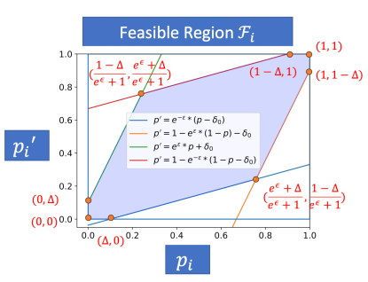
Proof.
Part I: Reducing # privacy constraints from to exponentially many.
Consider for an arbitrary and fixing . Given any noise function , recall the privacy cost objective (see Lemma 3.4), is
and the privacy constraints are of the form
where recall that is a function of and is a function of , and , are the sum of observed outcomes on neighboring datasets and . By Lemma 3.4, needs to make the above privacy constraint hold for all possible to make -differentially private. This is equivalent to saying, needs to ensure .
Notice that the sum of observed outcomes follows a Poisson Binomial distribution, i.e., and . Hence, by the pmf of the Poisson Binomial distribution666See, e.g. https://en.wikipedia.org/wiki/Poisson_binomial_distribution, for the pmf of Poisson Binomial distribution. , the privacy cost objective is linear in each and , fixing all , . Since each mechanism is -differentially private, by definition, satisfies all of the following:
That is, lies in a feasible region (see Figure 5). Note the constraints on , that is, the boundaries of , are linear in and . And so the optimization problem , which finds the worst case probabilities in , is a Linear Programming (LP) problem in for . This implies has to be on one of the eight corners of — that is , . Since all and , for , are independent, we can search for the worst case probabilities by searching for , instead of searching for . Therefore, the infinitely many privacy constraints are now reduced to only to optimize for the best function that maximizes the utility of , while ensuring the output is -differentially private.
Part II: Reducing # privacy constraints from exponentially many to a polynomial set.
To further reduce the number of privacy constraints in optimization, observe that the Poisson Binomial distribution is invariant under the permutation of its parameters. That is, , for some permutation and means “follows the same distribution”. Similarly, .
The above observation implies if we have one privacy constraint , for some , then any privacy constraint , where , , for permutations and , is redundant.
Therefore, there is a vector set , where each probability vector in is constructed by setting , where , such that vectors constructed by is not in . Note (8 chooses K with replacement) = . If we can restrict our search for the worst case probabilities to this set — that is, solving for , then . This implies we only need privacy constraints to optimize for the best noise function in DaRRM, while making sure is -differentially private.
Note if , i.e., the mechanism ’s are pure differentially private, the feasible region in which lies has only 4 corners instead of 8. This implies . Hence, in this case, (4 choose with replacement) = , which implies we only need privacy constraints to optimize for the best noise function in DaRRM.
∎
Appendix D Full Experiment Results
D.1 Optimized in Simulations
D.1.1 Comparison Using General Composition
The general composition (Theorem 2.3) indicates less total privacy loss than simple composition (Theorem 2.2) when the number of folds, , is large, or when the failure probability is large. To enable meaningful comparison against general composition, we consider a larger and a larger failure probability .
Consider . By general composition, if one outputs the majority of subsampled mechanisms for some , the majority output is -differentially private, where
for some . We set this as the privacy guarantee of all majority ensembling algorithms. That is, if we want the majority output to be -differentially private, we set
and accordingly. The parameters and to compute in RR (see Section A.1) are set to be
and .
In the experiments, we consider and ; and is computed using a uniform prior .
All values of the parameters of the private ensembling algorithms we use in the experiment are listed in the table:
| # Subsampled mechanisms | 10 | 13 | 15 | 20 | |
| Privacy allowance | 6.4521 | 7.5742 | 8.2708 | 9.8823 | |
| Parameter of constant | 14.0328 | 14.0328 | 14.0328 | 14.0328 | |
| Parameter of constant | 0.1003 | 0.1003 | 0.1003 | 0.1003 | |
| Overall privacy loss | 0.6452 | 0.7574 | 0.8271 | 0.9882 | |
| Overall failure probability | 0.1001 | 0.1001 | 0.1001 | 0.1002 |
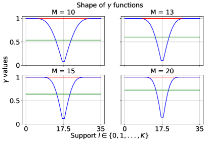
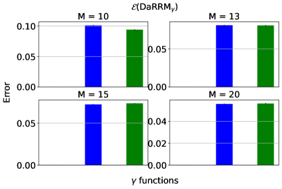

D.1.2 Comparison in Pure Differential Privacy Settings
Consider the pure differential privacy setting, where . Note in this setting, it is known that simple composition is tight.
To compute an optimized in DaRRM, since we have shown the number of constraints is if (see Lemma 5.1), we can set to be larger. Here, we present results for and .
Again, we compare the shape of different and the corresponding under those functions, fixing the total privacy loss to be . is computed using a uniform prior .
Since the subsampling mechanism from Section 4 with privacy amplification applies to this setting, we compare four different noise functions here:
-
1.
(Ours): optimized function using our optimization framework
-
2.
(Baseline): the function that corresponds to outputting the majority of out subsampled mechanisms
-
3.
(Baseline): the function that corresponds to outputting subsampled mechanisms from Theorem 4.1, aka., Double Subsampling (DSub)
-
4.
(Baseline): the constant function that corresponds to the classical Randomized Response (RR) algorithm
Setting 1. , .
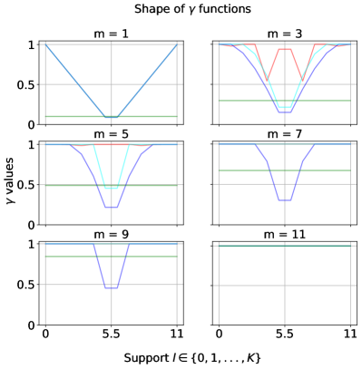
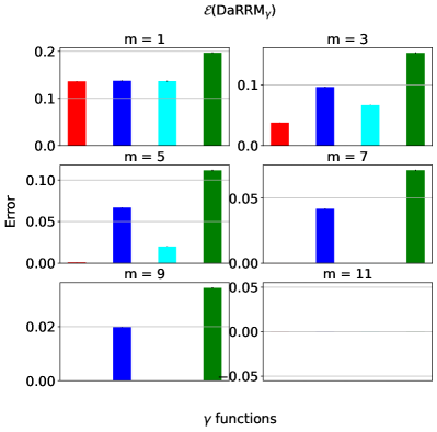

Setting 2. .
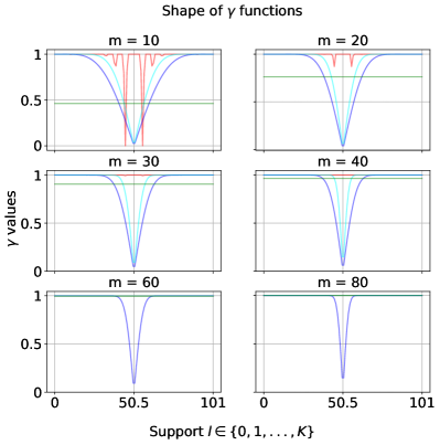
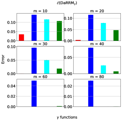

D.1.3 Comparison Using Different Prior Distributions
When optimizing that maximizes the utility in DaRRM, recall that the objective takes an expectation over ’s for , where is some distribution and . The previous experiments assume we do not have access to any prior knowledge about ’s and hence is the uniform distribution, i.e., . However, when one has knowledge about the mechanisms, one can set a proper prior to further maximize the utility of DaRRM.
In this section, let denote and we present results considering a different prior distribution, which we call , as follows. Suppose our prior belief is that each mechanism has a clear tendency towards voting 0 or 1, i.e., is far from 0.5. Let be Uniform().
To optimize under , we change the approximate optimization objective in Eq. 202, which optimizes under , to be the following,
| (204) |
Setting. , , .
We compare the shape and of different functions:
-
1.
denote the function optimized under
-
2.
denote the function optimized under
-
3.
, corresponding to the subsampling baseline
-
4.
, corresponding to the RR baseline
Note when we compute the error, we take the expectation w.r.t. the actual distributions, regardless of the prior used to optimize . In the experiments, we consider three different actual distributions:"
-
1.
“Actual: Uniform”:
-
2.
“Actual: ”:
This setting implies the mechanisms do not have a clear majority
-
3.
“Actual: Uniform”:
This setting implies the mechanisms have a clear majority (i.e., 0)
Since our prior is closer to (i.e., there is a clear majority), we would expect to be the lowest when , but to be higher than when or . The results are presented in Figure 9.
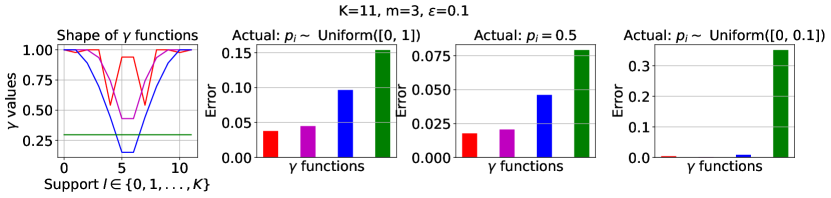
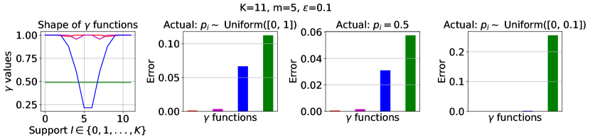

D.2 Private Semi-Supervised Knowledge Transfer
D.2.1 More Details about the Baseline GNMax Papernot et al. (2018)
The GNMax aggregation mechanism for majority ensembling of non-private teachers proceeds as follows (Section 4.1 of Papernot et al. (2018)): on input ,
| (205) |
where is # teachers who vote for class .
How to set in GNMax?
Section 4.1 of Papernot et al. (2018) states the GNMax mechanism is -Renyi differentially private (RDP), for all . RDP bounds can be converted to DP bounds as follows:
Theorem D.1 (RDP to DP (Theorem 5 of Papernot et al. (2018))).
If a mechanism guarantees -RDP, then guarantees -differential privacy for .
Therefore, GNMax with parameter guarantees -differential privacy, . Given , we want to choose and here so that the output of GNMax is -differentially private. Here, .
We first obtain a valid range of . Since , and so . And . Since the smaller is, the higher the utility, we perform a grid search over , with discretized values of equal distance 0.5, to find the minimum . For the values used in the experiments, we observe decreases first and then increases as increases, as shown in Figure 10. The and values in the RDP bound of Gaussian noise to compute the privacy loss of GNMax’s output we use in the experiments are presented in Table 4.
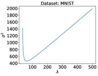
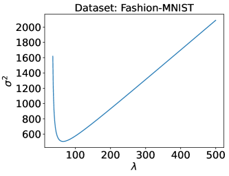
| Privacy Loss Per Query | |||
|---|---|---|---|
| MNIST | 34.31 | 21.46 | |
| Fashion-MNIST | 35.74 | 22.46 |
A Note on the Data-dependent Privacy Loss Bound
Papernot et al. (2018) gives a potentially tighter data-dependent bound on the privacy loss using GNMax to output the majority of non-private teacherss votes. We give a clean pseudo-code on computing the data-dependent privacy loss bound in Algorithm 6, based on the lemmas and theorems in Papernot et al. (2018). Given privacy parameters and the teacher votes per class for classes, the data-dependent bound can be empirically evaluated and compared against the Gaussian privacy loss bound. The smaller one is the final privacy loss. We empirically find that the condition of the data-dependent bound (line 8 in Algorithm 6) is not satisfied when and the number of classes are small, e.g., as in our case, even if all teachers agree on the same output. And so in the experiments, we can only apply the Gaussian privacy loss bound (line 14).
D.2.2 Additional Results for Private Semi-Supervised Knowledge Transfer
.
| Dataset | # Queries | Privacy loss per query | Total privacy loss over queries |
|---|---|---|---|
| MNIST | |||
| Fashion MNIST | |||
Dataset MNIST # Queries GNMax (Baseline) (Baseline) (Ours) 0.54 (0.11) 0.68 (0.07) 0.74 (0.08) 0.51 (0.07) 0.67 (0.05) 0.66 (0.05) 0.57 (0.03) 0.71 (0.03) 0.69 (0.04)
Dataset Fashion-MNIST # Queries GNMax (Baseline) (Baseline) (Ours) 0.56 (0.10) 0.92 (0.05) 0.89 (0.06) 0.52 (0.05) 0.89 (0.04) 0.92 (0.03) 0.56 (0.04) 0.89 (0.04) 0.91 (0.04)
.
| Dataset | # Queries | Privacy loss per query | Total privacy loss over queries |
|---|---|---|---|
| MNIST | |||
| Fashion MNIST | |||
Dataset MNIST # Queries GNMax (Baseline) (Baseline) (Ours) 0.73 (0.11) 0.76 (0.09) 0.84 (0.07) 0.75 (0.07) 0.82 (0.04) 0.83 (0.04) 0.72 (0.04) 0.79 (0.05) 0.83 (0.03)
Dataset Fashion-MNIST # Queries GNMax (Baseline) (Baseline) (Ours) 0.72 (0.10) 0.96 (0.04) 0.97 (0.04) 0.72 (0.08) 0.96 (0.02) 0.97 (0.02) 0.72 (0.06) 0.97 (0.01) 0.97 (0.01)
.
| Dataset | # Queries | Privacy loss per query | Total privacy loss over queries |
|---|---|---|---|
| MNIST | |||
| Fashion MNIST | |||
Dataset MNIST # Queries GNMax (Baseline) (Baseline) (Ours) 0.79 (0.07) 0.80 (0.09) 0.85 (0.08) 0.80 (0.05) 0.82 (0.05) 0.85 (0.04) 0.80 (0.04) 0.80 (0.04) 0.83 (0.03)
Dataset Fashion-MNIST # Queries GNMax (Baseline) (Baseline) (Ours) 0.79 (0.07) 0.95 (0.04) 0.96 (0.04) 0.79 (0.05) 0.96 (0.03) 0.97 (0.03) 0.79 (0.03) 0.96 (0.02) 0.96 (0.02)