Optimizing distortion riskmetrics with distributional uncertainty

Silvana M. Pesenti Department of Statistical Sciences, University of Toronto, Canada. ✉ silvana.pesenti@utoronto.ca Qiuqi Wang Department of Statistics and Actuarial Science, University of Waterloo, Canada. ✉ q428wang@uwaterloo.ca Ruodu Wang Department of Statistics and Actuarial Science, University of Waterloo, Canada. ✉ wang@uwaterloo.ca

Abstract

Optimization of distortion riskmetrics with distributional uncertainty has wide applications in finance and operations research. Distortion riskmetrics include many commonly applied risk measures and deviation measures, which are not necessarily monotone or convex. One of our central findings is a unifying result that allows us to convert an optimization of a non-convex distortion riskmetric with distributional uncertainty to a convex one, leading to great tractability. A sufficient condition to the unifying equivalence result is the novel notion of closedness under concentration, a variation of which is also shown to be necessary for the equivalence. Our results include many special cases that are well studied in the optimization literature, including but not limited to optimizing probabilities, Value-at-Risk, Expected Shortfall, Yaari’s dual utility, and differences between distortion risk measures, under various forms of distributional uncertainty. We illustrate our theoretical results via applications to portfolio optimization, optimization under moment constraints, and preference robust optimization.

Keywords: risk measures; deviation measures; distributionally robust optimization; convexification; conditional expectation

1 Introduction

Riskmetrics, such as measures of risk and variability, are common tools to represent preferences, model decisions under risks, and quantify different types of risks. To fix terms, we refer to riskmetrics as any mapping from a set of random variables to the real line, and risk measures as riskmetrics that are monotone in the sense of Artzner et al. (1999).

In this paper, we focus on distortion riskmetrics which is a large class of commonly used measures of risk and variability; see Wang et al. (2020a) for the terminology “distortion riskmetrics”. Distortion riskmetrics include L-functionals (Huber and Ronchetti, 2009) in statistics, Yaari’s dual utilities (Yaari, 1987) in decision theory, distorted premium principles (Wang et al., 1997) in insurance, and spectral risk measures (Acerbi, 2002) in finance; see Wang et al. (2020a) for further examples. After a normalization, increasing distortion riskmetrics are distortion risk measures, which include, in particular, the two most important risk measures used in current banking and insurance regulation, the Value-at-Risk (VaR) and the Expected Shortfall (ES). Moreover, convex distortion riskmetrics are the building blocks (via taking a supremum) for all convex risk functionals (Liu et al., 2020), including classic risk measures (Artzner et al., 1999; Föllmer and Schied, 2002) and deviation measures (Rockafellar et al., 2006).

When riskmetrics are evaluated on distributions that are subject to uncertainty, decisions should be taken with respect to the worst (or best) possible values a riskmetric attains over a set of alternative distributions; giving rise to the active subfield of distributionally robust optimization. The set of alternative distributions, the uncertainty set, may be characterized by moment constraints (e.g., Popescu (2007)), parameter uncertainty (e.g., Delage and Ye (2010)), probability constraints (e.g., Wiesemann et al. (2014)), and distributional distances (e.g., Blanchet and Murthy (2019)), amongst others. Popular distortion risk measures such as VaR and ES are studied extensively in this context; see e.g., Natarajan et al. (2008) and Zhu and Fukushima (2009).

Optimization of convex distortion risk measures, i.e., distortion riskmetrics with an increasing and concave distortion function, is relatively well understood under distributional uncertainty; see Cornilly et al. (2018), Li (2018), and Liu et al. (2020) for some recent work. Nevertheless, many distortion riskmetrics are not convex or monotone. For example, in the Cumulative Prospect Theory of Tversky and Kahneman (1992), the distortion function is typically assumed to be inverse-S-shaped; in financial risk management, the popular risk measure $\mathrm{VaR}$ has a non-concave distortion function, and the inter-quantile difference (Wang et al., 2020b) has a distortion function that is neither concave nor monotone. Another example is the difference between two distortion risk measures, which is clearly not increasing or convex in general. Optimizing non-convex distortion riskmetrics under distributional uncertainty is difficult and results are available only for special cases; see Li et al. (2018), Cai et al. (2018), Zhu and Shao (2018), Wang et al. (2019), and Bernard et al. (2020), all with an increasing distortion function.

There is, however, a notable common feature in the above mentioned literature when a non-convex distortion risk metric is involved. For numerous special cases, one often obtains an equivalence between the optimization problem with non-convex distortion riskmetric and that with a convex one. Inspired by this observation, the aim of this paper is to address:

What conditions provide equivalence between a non-convex riskmetric and a convex one in the setting of distributional uncertainty?

An answer to this question is still missing in the literature. In this sense, we offer a novel perspective on distributionally robust optimization problems by converting non-convex optimization problems to their convex counterpart. Transforming a non-convex to a convex optimization problem through approximation and via a direct equivalence has been studied by Zymler et al. (2013) and Cai et al. (2020). Both contributions, however, consider uncertainty sets described by some special forms of constraints. A unifying framework applicable to numerous uncertainty sets and the entire class of distortion riskmetrics is however missing and at the core of this paper.

The main novelty of our results is three-fold: first, we obtain a unifying result (Theorem 1) that allows, under distributional uncertainty, to convert an optimization problem of a non-convex distortion riskmetric to an optimization problem with a convex one. The result covers, to the authors’ best knowledge, all known equivalences between optimization problems of non-convex and convex riskmetrics with distributional uncertainty. The proof requires techniques beyond the ones used in the existing literature, as we do not make assumptions such as monotonicity, positiveness, and continuity. Our framework can also be easily applied to settings with atomic probability space or with uncertainty sets of multi-dimensional distributions. Second, we introduce the concept of closedness under concentration as a sufficient condition to establish the equivalence, and it is also a necessary condition on the set of optimizers given that the equivalence holds (Theorem 2). We show how the properties of closedness under concentration within a collection of intervals $\mathcal{I}$ and closedness under concentration for all intervals can easily be verified and provide numerous examples. Third, the classes of distortion riskmetrics and uncertainty formulations considered in this paper include all special cases studied in the literature; examples are presented in Sections 3-4. In particular, our class of riskmetrics include all practically used risk measures and variability measures (some via taking a sup), dual utilities with inverse-S-shaped distortion functions of Tversky and Kahneman (1992), and differences between two dual utilities or distortion risk measures. Our uncertainty formulations include both supremum and infimum problems,¹¹1Thus we provide a universal treatment of worst-case and best-case risk values. Calculating best-case risk values allows us to solve economic decision making problems where optimal distributions are chosen to minimize the risk. moment constraints, convex order/risk measure constraints, marginal constraints in risk aggregation with dependence uncertainty (e.g., Embrechts et al. (2015)), preference robust optimization (e.g., Armbruster and Delage (2015) and Guo and Xu (2021)), and some one-dimensional and multi-dimensional uncertainty sets induced by Wasserstein metrics.

The great generality distinguishes our work from the large literature on distributional robust optimization cited above. Our work is of analytical and probabilistic nature, and we focus on theoretical equivalence results which will be also illustrated via numerical implementations. The target problems are formulated in Section 2. Sections 3 is devoted to our main contribution of the equivalence of non-convex and convex optimization problems with distributional uncertainty. We illustrate by many examples the concepts of closedness under conditional expectation and closedness under concentration, and distinguish them in several practical settings. Section 4 demonstrates the equivalence results in multi-dimensional settings. In addition to a general multi-dimensional model with a concave loss function, we solve a robust risk aggregation problem with ambiguity on both the marginal distributions and the dependence structure. In Section 5, our results are used to solve optimization problems with uncertainty sets defined via moment constraints. In particular, we generalize a few well-known results in the literature on optimization and worst-case values of risk measures. Sections 6 and 7 contain numerical illustrations of optimizing differences between two distortion riskmetrics, portfolio optimization, and preference robust optimization. Some concluding remarks are put in Section 8. Proofs of all results are relegated to Appendix B.

2 Distortion riskmetrics with distributional uncertainty

2.1 Problem formulation

Throughout, we work with an atomless probability space $(\Omega,\mathscr{F},\mathbb{P})$ . For $n\in\mathbb{N}$ , $A$ represents a set of actions, $\rho$ is an objective functional, $f:A\times\mathbb{R}^{n}\to\mathbb{R}$ is a loss function, and $\mathbf{X}$ is an $n$ -dimensional random vector with distributional uncertainty. Many problems in distributionally robust optimization have the form

\min_{\mathbf{a}\in A}\,\sup_{F_{\mathbf{X}}\in\widetilde{\mathcal{M}}}\;\rho(f(\mathbf{a},\mathbf{X})),

(1)

where $F_{\mathbf{X}}$ denotes the distribution of $\mathbf{X}$ and $\widetilde{\mathcal{M}}$ is a set of plausible distributions for $\mathbf{X}$ . We will first focus on the inner problem

\sup_{F_{\mathbf{X}}\in\widetilde{\mathcal{M}}}\;\rho(f(\mathbf{a},\mathbf{X})),

(2)

which we may rewrite as

\sup_{F_{Y}\in\mathcal{M}}\rho(Y),

(3)

where $F_{Y}$ denotes the distribution of $Y$ and $\mathcal{M}$ is a set of distributions on $\mathbb{R}$ . We suppress the reliance on $\mathbf{a}$ as it remains constant in the inner problem (2). The supremum in (3) is typically referred to as the worst-case risk measure in the literature if $\rho$ is monotone.²²2A risk measure $\rho:\mathcal{L}^{p}\to\mathbb{R}$ is monotone if $\rho(X)\leqslant\rho(Y)$ for all $X,Y\in\mathcal{L}^{p}$ with $X\leqslant Y$ . The problem (3) can also represent an optimal decision problem, where $\rho$ is an objective to maximize, and a decision maker chooses an optimal distribution from the set $\mathcal{M}$ which is interpreted as an action set instead of an uncertainty set (i.e., no uncertainty in this problem). Since the two problems share the same mathematical formulation (3), we will navigate through our results mainly with the first interpretation of worst-case risk under uncertainty.

We denote by $\mathcal{L}^{p}$ , $p\in[1,\infty)$ , the space of random variables with finite $p$ -th moment. Let $\mathcal{L}^{\infty}$ represent the set of bounded random variables and let $\mathcal{L}^{0}$ represent the space of all random variables. Denote by $\mathcal{H}$ the set of functions $h:[0,1]\mapsto\mathbb{R}$ with bounded variation satisfying $h(0)=0$ . For $p\in[1,\infty]$ and $h\in\mathcal{H}$ , a distortion riskmetric $\rho_{h}:\mathcal{L}^{p}\to\mathbb{R}$ is defined as

\rho_{h}(Y)=\int_{0}^{\infty}h(\mathbb{P}(Y>x))\,\mathrm{d}x+\int_{-\infty}^{0}(h(\mathbb{P}(Y>x))-h(1))\,\mathrm{d}x,~{}~{}Y\in\mathcal{L}^{p},

(4)

whenever the above integrals are finite; see Proposition 5 below for a sufficient condition. The function $h\in\mathcal{H}$ is called a distortion function. Note that we allow $h$ to be non-monotone; if $h$ is increasing and $h(1)=1$ , then $\rho_{h}$ is a distortion risk measure. The distortion riskmetric $\rho_{h}$ is convex if and only if $h$ is concave; see Wang et al. (2020b) for this and other properties of $\rho_{h}$ .

In this paper we consider the objective functional $\rho$ in (1) to be a distortion riskmetric $\rho_{h}$ for some $h\in\mathcal{H}$ , as the class of distortion riskmetrics includes a large class of objective functionals of interest. Note that a general analysis of (3) also covers the infimum problem $\inf_{F_{Y}\in\mathcal{M}}\rho_{h}(Y)$ , since $-\rho_{h}=\rho_{-h}$ is again a distortion riskmetric. This illustrates an advantage of studying distortion riskmetrics over monotone ones, as our analysis unifies best- and worst-case risk evaluations. Best-case risk measures are also of practical importance. In particular, they may represent risk minimization problems through the second interpretation of (3), where $\mathcal{M}$ represents a set of possible actions (see Section 3.4 for some examples).

If $\rho_{h}$ is not convex, or equivalently, $h$ is not concave, optimization problems of the type (3) are often highly nontrivial. However, the optimization problem of maximizing $\rho_{h^{*}}(Y)$ over ${F_{Y}\in\mathcal{M}}$ , where $h^{*}$ is the smallest concave distortion function dominating $h$ , is convex and can often be solved relatively easily either analytically or through numerical methods. Clearly, since $\rho_{h^{*}}\geqslant\rho_{h}$ , we have

\sup_{F_{Y}\in\mathcal{M}}\rho_{h}(Y)\leqslant\sup_{F_{Y}\in\mathcal{M}}\rho_{h^{*}}(Y)

and one naturally wonders when the above inequality holds as equality, that is, under what conditions, it holds

\sup_{F_{Y}\in\mathcal{M}}\rho_{h}(Y)=\sup_{F_{Y}\in\mathcal{M}}\rho_{h^{*}}(Y)\,.

(5)

The main contribution of this paper is a sufficient condition on the uncertainty set $\mathcal{M}$ that guarantees equivalence of these optimization problems, that is (5) holds. We will also obtain a necessary condition. If (5) holds, then the non-convex problem (the left-hand side of (5)) is converted into the convex problem (the right-hand side of (5)), providing huge convenience, which in turn helps to solve the minimax problem (1).

2.2 Notation and preliminaries

For $p\geqslant 1$ and $n\in\mathbb{N}$ , we denote by $\mathcal{M}^{n}_{p}$ the set of all distributions on $\mathbb{R}^{n}$ with finite $p$ -th moment. Let $\mathcal{M}^{n}_{\infty}$ be the set of $n$ -dimensional distributions of bounded random variables. For $p\in[1,\infty]$ , write $\mathcal{M}^{1}_{p}=\mathcal{M}_{p}$ for simplicity. The set inclusion $\subset$ and terms like “increasing” and “decreasing” are in the non-strict sense. For $X,Y\in\mathcal{L}^{p}$ , we write $X\buildrel\mathrm{d}\over{=}Y$ to represent that $X$ and $Y$ have the same distribution. For a distribution $F\in\mathcal{M}_{1}$ , let its left- and right-quantile functions be given respectively by

F^{-1}(\alpha)=\inf\>\{x\in\mathbb{R}:F(x)\geqslant\alpha\}~{}~{}\text{and}~{}~{}F^{-1+}(\alpha)=\inf\>\{x\in\mathbb{R}:F(x)>\alpha\},~{}~{}\alpha\in[0,1],

with the convention $\inf(\varnothing)=\infty$ . For $x,y\in\mathbb{R}$ , we write $x\vee y=\max\{x,y\}$ and $x\wedge y=\min\{x,y\}$ . Since $h\in\mathcal{H}$ is of bounded variation, its discontinuity points are at most countable and the left- and right-limits exist at each of these points. We write

h(t^{+})=\left\{\begin{array}[]{l l}\lim_{x\downarrow t}h(x),&t\in[0,1),\\ h(1),&t=1,\end{array}\right.~{}~{}\text{and}~{}~{}h(t^{-})=\left\{\begin{array}[]{l l}\lim_{x\uparrow t}h(x),&t\in(0,1],\\ h(0),&t=0,\end{array}\right.

and the upper semicontinuous modification of $h$ is denoted by

\hat{h}(t)=h(t^{+})\vee h(t^{-})\vee h(t),~{}~{}t\in(0,1),~{}~{}\mbox{with }\hat{h}(0)=0~{}\mbox{and}~{}\hat{h}(1)=h(1).

Note that $\hat{h}(t)=h(t)$ at all continuous points of $h$ , and we do not make any modification at the points $0$ and $1$ even if $h$ has a jump at these points. For $h\in\mathcal{H}$ and $t\in[0,1]$ , define its concave and convex envelopes $h^{*}$ and $h_{*}$ respectively by

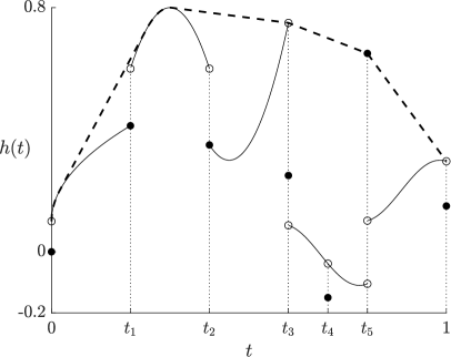
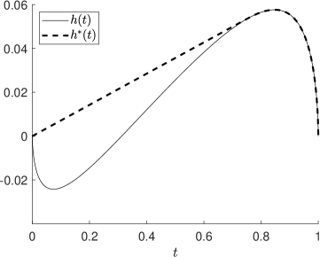
h^{*}(t)=\inf\left\{g(t):~{}g\in\mathcal{H},~{}g\geqslant h,~{}g\textrm{ is concave on}~{}[0,1]\right\},

h_{*}(t)=\sup\left\{g(t):~{}g\in\mathcal{H},~{}g\leqslant h,~{}g\textrm{ is convex on}~{}[0,1]\right\}.

Both $h^{*}$ and $h_{*}$ are continuous functions on $(0,1)$ for all $h\in\mathcal{H}$ , and if $h$ is continuous at $0$ and $1$ , then so are $h^{*}$ and $h_{*}$ (see Figure 4 below for an illustration of $h$ and $h^{*}$ ). Denote by $\mathcal{H}^{*}$ (resp. $\mathcal{H}_{*}$ ) the set of concave (resp. convex) functions in $\mathcal{H}$ . Note that for all $h\in\mathcal{H}$ , we have $h^{*}\in\mathcal{H}^{*}$ and $h_{*}\in\mathcal{H}_{*}$ . As a well-known property of the convex and concave envelopes of a continuous $h$ (e.g., Brighi and Chipot (1994)), $h^{*}$ (resp. $h_{*}$ ) differs from $h$ on a union of disjoint open intervals, and $h^{*}$ (resp. $h_{*}$ ) is linear on these intervals. The functions $h$ , $\hat{h}$ , $h^{*}$ and $(\hat{h})^{*}$ are illustrated in Figure 1.

Refer to caption — Figure 1: An example of $h$ (left) and $\hat{h}$ (right) with the set of discontinuity points $\{t_{1},t_{2},t_{3},t_{4},t_{5}\}$ excluding $0$ and $1$ ; the dashed lines represent $h^{*}$ and $(\hat{h})^{*}$ , which are identical by Proposition 1

While in general $\rho_{h}$ and $\rho_{\hat{h}}$ are different functionals, one has $\rho_{h}(Y)=\rho_{\hat{h}}(Y)$ for any random variable $Y$ with continuous quantile function; see Lemma 1 of Wang et al. (2020a). Moreover, $h^{*}=(\hat{h})^{*}\geqslant\hat{h}\geqslant h$ and the four functions are all equal if $h$ is concave. Below, we provide a new result on convex envelopes of distortion functions $h$ that are not necessarily monotone or continuous, which may be of independent interest.

Proposition 1.

For any $h\in\mathcal{H}$ , we have $h^{*}=(\hat{h})^{*}$ and the set $\{t\in[0,1]:\hat{h}(t)\neq h^{*}(t)\}$ is the union of some disjoint open intervals. Moreover, $h^{*}$ is linear on each of the above intervals.

In the sequel, we mainly focus on $h^{*}$ , which will be useful when optimizing $\rho_{h}$ in (3). A similar result to Proposition 1 holds for $h_{*}$ , useful in the corresponding infimum problem, where the upper semicontinuous modification of $h$ is replaced by the lower semicontinuous one. This follows directly from Proposition 1 by setting $g=-h$ which gives $\rho_{g}=-\rho_{h}$ and $h_{*}=-g^{*}$ .

For all distortion functions $h\in\mathcal{H}$ , from Proposition 1, there exist (countably many) disjoint open intervals on which $\hat{h}\neq h^{*}$ . Using a similar notation to Wang et al. (2019), we define the set

\mathcal{I}_{h}=\{(1-b,1-a):\hat{h}\neq h^{*}\text{ on }(a,b),~{}\hat{h}(a)=h^{*}(a),~{}\hat{h}(b)=h^{*}(b)\}\,.

The set $\mathcal{I}_{h}$ is easy to identify in practice; see Section 3.2 for examples of commonly used distortion riskmetrics and their corresponding sets $\mathcal{I}_{h}$ .

3 Equivalence between non-convex and convex riskmetrics

3.1 Concentration and the main equivalence result

In this section, we introduce the concept of concentration, and use this concept to explain our main equivalence results, Theorems 1 and 2. For a distribution $F\in\mathcal{M}_{1}$ and an interval $C\subset[0,1]$ (when speaking of an interval in $[0,1]$ , we exclude singletons or empty sets), we define the $C$ -concentration of $F$ , denote by $F^{C}$ , as the distribution of the random variable

F^{-1}(U)\mathds{1}_{\{U\not\in C\}}+\mathbb{E}[F^{-1}(U)|U\in C]\mathds{1}_{\{U\in C\}},

(6)

where $U\sim\mathrm{U}[0,1]$ is a standard uniform random variable. In other words, $F^{C}$ is obtained by concentrating the probability mass of $F^{-1}(U)$ on $\{U\in C\}$ at its conditional expectation, whereas the rest of the distribution remains unchanged. For $F\in\mathcal{M}_{1}$ and $0\leqslant a<b\leqslant 1$ , it is clear that the left-quantile function of $F^{(a,b)}$ is given by

F^{-1}(t)\mathds{1}_{\{t\not\in(a,b]\}}+\frac{\int_{a}^{b}F^{-1}(u)\,\mathrm{d}u}{b-a}\mathds{1}_{\{t\in(a,b]\}},~{}~{}t\in[0,1].

(7)

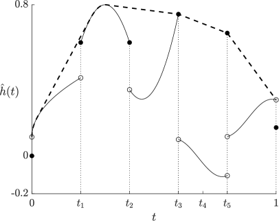
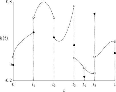
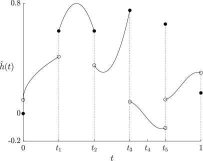
For a collection $\mathcal{I}$ of (possibly infinitely many) non-overlapping intervals in $[0,1]$ , let $F^{\mathcal{I}}$ be the distribution corresponding to the left-quantile function given by the left-continuous version of

F^{-1}(t)\mathds{1}_{\{t\not\in\bigcup_{C\in\mathcal{I}}C\}}+\sum_{C\in\mathcal{I}}\frac{\int_{C}F^{-1}(u)\,\mathrm{d}u}{\lambda(C)}\mathds{1}_{\{t\in C\}},~{}~{}~{}~{}t\in[0,1],

(8)

where $\lambda$ is the Lebesgue measure; see Figure 2 for an illustration.

Figure 2: Left panel: quantile function of

F

; right panel: quantile function of

F^{\mathcal{I}}

where

\mathcal{I}=\{(0,1/3),(1/2,2/3)\}

Definition 1.

Let $\mathcal{M}$ be a set of distributions in $\mathcal{M}_{1}$ and $\mathcal{I}$ be a collection $\mathcal{I}$ of intervals in $[0,1]$ . We say that (a) $\mathcal{M}$ is closed under concentration within $\mathcal{I}$ if $F^{\mathcal{I}}\in\mathcal{M}$ for all $F\in\mathcal{M}$ ; (b) $\mathcal{M}$ is closed under concentration for all intervals if for all $F\in\mathcal{M}$ , we have $F^{C}\in\mathcal{M}$ for all intervals $C\subset[0,1]$ ; (c) $\mathcal{M}$ is closed under conditional expectation if for all $F_{X}\in\mathcal{M}$ , the distribution of any conditional expectation of $X$ is in $\mathcal{M}$ .

The relationship between the three properties of closedness in Definition 1 is discussed in Propositions 2 and 3 below. Generally, (c) $\Rightarrow$ (b) $\Rightarrow$ (a) if $\mathcal{I}$ is finite. Our main equivalence result is summarized in the following theorem.

Theorem 1.

For $\mathcal{M}\subset\mathcal{M}_{1}$ and $h\in\mathcal{H}$ , the following hold.

(i)

If $h=\hat{h}$ , i.e., $h$ is upper semicontinuous on $(0,1)$ , and $\mathcal{M}$ is closed under concentration within $\mathcal{I}_{h}$ , then

$\sup_{F_{Y}\in\mathcal{M}}\rho_{h}(Y)=\sup_{F_{Y}\in\mathcal{M}}\rho_{h^{*}}(Y).$ (9)
(ii)

If $\mathcal{M}$ is closed under concentration for all intervals, then (9) holds.
(iii)

If $h=\hat{h}$ , $\mathcal{M}$ is closed under concentration within $\mathcal{I}_{h}$ , and the second supremum in (9) is attained by some $F\in\mathcal{M}$ , then $F^{\mathcal{I}_{h}}$ attains both suprema.

Both suprema in (9) may be infinite, and this is discussed in Remark 5 in Appendix A.2. The proof of Theorem 1 is more technical than similar results in the literature because of the challenges arising from non-monotonicity, non-positivity, and discontinuity of $h$ ; see Figure 1 for a sample of possible complications. In (ii), $h$ does not need to be upper semicontinuous on $(0,1)$ for (9) to hold because closedness under concentration for all intervals in (ii) is stronger than the condition in (i).

Remark 1.

For $\mathcal{M}\subset\mathcal{M}_{1}$ and $h\in\mathcal{H}$ , if $h=\hat{h}$ and $F^{C}\in\mathcal{M}$ for all $F\in\mathcal{M}$ and $C\in\mathcal{I}_{h}$ , then the equivalence relation (9) also holds. If $\mathcal{I}_{h}$ is finite, then this condition is generally stronger than closedness under concentration within $\mathcal{I}_{h}$ in (i).

A natural question from Theorem 1 is whether our key condition of closedness under concentration is necessary in some sense for the equivalence (9) to hold.³³3We thank an anonymous referee for raising this question. It is immediate to notice that adding any distributions $F_{Z}$ satisfying $\rho_{h^{*}}(Z)<\sup_{F_{Y}\in\mathcal{M}}\rho_{h^{*}}(Y)$ to the set $\mathcal{M}$ does not affect the equivalence, and therefore we turn our attention to the set of maximizers instead of the whole set $\mathcal{M}$ . In the next result, we show that closedness under concentration within $\mathcal{I}_{h}$ of the set of maximizers of (3) is necessary for the equivalence (9) to hold.

Theorem 2.

For $\mathcal{M}\subset\mathcal{M}_{1}$ and $h\in\mathcal{H}$ such that $h\neq h^{*}$ , suppose that the set $\mathcal{M}_{\mathrm{opt}}$ of all maximizers of $\max_{F_{Y}\in\mathcal{M}}\rho_{h}(Y)$ is non-empty. If the equivalence (9) holds, i.e., $\sup_{F_{Y}\in\mathcal{M}}\rho_{h}(Y)=\sup_{F_{Y}\in\mathcal{M}}\rho_{h^{*}}(Y)$ , then $\mathcal{M}_{\mathrm{opt}}$ is closed under concentration within $\mathcal{I}_{h}$ .

If the equivalence (9) holds, then each $F\in\mathcal{M}_{\mathrm{opt}}$ also maximizes the problem $\sup_{F_{Y}\in\mathcal{M}}\rho_{h^{*}}(Y)$ . Conversely, if $h=\hat{h}$ , then this condition and closedness of $\mathcal{M}_{\mathrm{opt}}$ under concentration within $\mathcal{I}_{h}$ together are necessary (by Theorem 2) and sufficient (by Theorem 1) for the equivalence (9) to hold. If the maximizer $F$ of the original problem (3) is unique, then by Theorem 2, $F$ must be equal to $F^{\mathcal{I}_{h}}$ . The equivalence (9) does not imply closedness under concentration within $\mathcal{I}_{h}$ of the uncertainty set $\mathcal{M}$ itself; an example showing this is discussed in Remark 2.

3.2 Some examples of distortion riskmetrics

We provide a few examples of distortion riskmetrics $\rho_{h}$ commonly used in decision theory and finance, and obtain their corresponding set $\mathcal{I}_{h}$ . The Value-at-Risk (VaR) and the Expected Shortfall (ES) are the most popular risk measures in practice. We introduce them first, followed by an inverse-S-shaped distortion function of Tversky and Kahneman (1992).

Example 1 (VaR and ES).

For $Y\in\mathcal{L}^{0}$ , using the sign convention of McNeil et al. (2015), VaR is defined as the left-quantile, and upper VaR ( $\mathrm{VaR}^{+}$ ) is defined as the right-quantile; that is,

\mathrm{VaR}_{\alpha}(Y)=F^{-1}_{Y}(\alpha),~{}~{}\alpha\in(0,1]~{}~{}~{}\mbox{and}~{}~{}~{}\mathrm{VaR}^{+}_{\alpha}(Y)=F^{-1+}_{Y}(\alpha),~{}~{}\alpha\in[0,1).

ES at level $\alpha$ is defined as

\mathrm{ES}_{\alpha}(Y)=\frac{1}{1-\alpha}\int_{\alpha}^{1}\mathrm{VaR}_{t}(Y)\,\mathrm{d}t,~{}~{}\alpha\in(0,1),~{}Y\in\mathcal{L}^{1}.

Both $\mathrm{VaR}_{\alpha}$ and $\mathrm{ES}_{\alpha}$ belong to the class of distortion riskmetrics. Take $\alpha\in(0,1)$ . Let $h(t)=\mathds{1}_{(1-\alpha,1]}(t)$ , $t\in[0,1]$ . It follows that $h\in\mathcal{H}$ and $\hat{h}(t)=\mathds{1}_{[1-\alpha,1]}(t)$ , $t\in[0,1]$ . In this case, $\rho_{h}=\mathrm{VaR}_{\alpha}$ . Moreover, $h^{*}(t)=\frac{t}{1-\alpha}\wedge 1$ , $t\in[0,1]$ and $\rho_{h^{*}}=\mathrm{ES}_{\alpha}$ . Since $h^{*}$ and $\hat{h}$ differ on $(0,1-\alpha),$ we have $\mathcal{I}_{h}=\{(\alpha,1)\}$ .

Example 2 (TK distortion riskmetrics).

The following function $h$ is an inverse-S-shaped distortion function (see also Figure 4):

h(t)=\frac{t^{\gamma}}{\left(t^{\gamma}+(1-t)^{\gamma}\right)^{1/\gamma}},~{}~{}t\in[0,1],~{}\gamma\in(0,1).

(10)

Distortion riskmetrics with distortion function (10) are commonly used in behavioural economics and finance; see e.g., Tversky and Kahneman (1992). For simplicity, we call such distortion riskmetrics TK distortion riskmetrics. Typical values of $\gamma$ are in $[0.5,0.9]$ ; see Wu and Gonzalez (1996). For $h$ in (10), it is clear that $h=\hat{h}$ on $[0,1]$ by continuity of $h$ . We have $h^{*}\neq h$ on $(t_{0},1)$ , for some $t_{0}\in(0,1)$ , and $h^{*}$ is linear on $[t_{0},1]$ . Thus, $\mathcal{I}_{h}=\{(0,1-t_{0})\}$ . An example of $h$ in (10) and its concave envelope $h^{*}$ are plotted in Figure 3 (left).

For $h_{1},h_{2}\in\mathcal{H}$ , we write $h=h_{1}-h_{2}\in\mathcal{H}$ and consider the difference between two distortion riskmetrics, that is

\rho_{h}=\rho_{h_{1}}-\rho_{h_{2}}.

(11)

Such type of distortion riskmetrics measure the difference or disagreement between two utilities, risk attitudes, or capital requirements. Determining the upper and lower bounds, or the largest absolute values of such measures of disagreement, is of interest in practice but rarely studied in the literature. Note that $h_{1}-h_{2}$ is in general not monotone or concave even when $h_{1}$ and $h_{2}$ themselves have the specified properties. Below we show some examples of distortion riskmetrics taking the form of (11).

Example 3 (Inter-quantile range and inter-ES range).

For $\alpha\in[1/2,1)$ , we take $h_{1}(t)=\mathds{1}_{[1-\alpha,1]}(t)$ and $h_{2}(t)=\mathds{1}_{(\alpha,1]}(t)$ , $t\in[0,1]$ . It follows that $h(t)=h_{1}(t)-h_{2}(t)=\mathds{1}_{\{1-\alpha\leqslant t\leqslant\alpha\}}$ , $t\in[0,1]$ , $\hat{h}=h$ , and

\rho_{h}(X)=F^{-1+}_{X}(\alpha)-F^{-1}_{X}(1-\alpha),~{}~{}X\in\mathcal{L}^{0}.

Correspondingly, we have $h^{*}(t)=t/(1-\alpha)\wedge 1+(\alpha-t)/(1-\alpha)\wedge 0$ , $t\in[0,1]$ , and

\rho_{h^{*}}(X)=\mathrm{ES}_{\alpha}(X)+\mathrm{ES}_{\alpha}(-X),~{}~{}X\in\mathcal{L}^{1}.

This distortion riskmetric $\rho_{h}$ is called an inter-quantile range and $\rho_{h^{*}}$ is called an inter-ES range. As the distortion functions $h^{*}$ and $\hat{h}$ differ on the open intervals $(0,1-\alpha)$ and $(\alpha,1)$ , we have $\mathcal{I}_{h}=\{(\alpha,1),(0,1-\alpha)\}$ . The distortion functions $h$ and $h^{*}$ are displayed in Figure 3 (right).

Example 4 (Difference of two inverse-S-shaped distortion functions).

We take $h_{1}$ and $h_{2}$ to be the inverse-S-shaped distortion functions in (10), with parameters $\gamma_{1}=0.8$ and $\gamma_{2}=0.7$ , respectively. By calculation, the function $h=h_{1}-h_{2}$ is convex on $[0,0.3770]$ , concave on $[0.3770,1]$ , and as seen in Figure 4 not monotone. The concave envelope $h^{*}$ is linear on $[0,0.7578]$ and $h^{*}=h$ on $[0.7578,1]$ . Thus, we have $\mathcal{I}_{h}=\{(0.2422,1)\}$ . The graphs of the distortion functions $h_{1}$ , $h_{2}$ , $h$ , and $h^{*}$ are displayed in Figure 4.

The functions in $\mathcal{H}$ are a.e. differentiable, and for an absolutely continuous function $h\in\mathcal{H}$ , let $h^{\prime}$ be a (representative) function on $[0,1]$ that is a.e. equal to the derivative of $h$ . If $h\in\mathcal{H}$ is left-continuous or $\mathrm{VaR}_{t}(Y)$ is continuous with respect to $t\in(0,1)$ , the risk measure $\rho_{h}$ in (4) has representation

\rho_{h}(Y)=\int_{0}^{1}\mathrm{VaR}_{1-t}(Y)\,\mathrm{d}h(t),~{}~{}Y\in\mathcal{L}^{p};

(12)

see Lemma 1 of Wang et al. (2020a). If $h\in\mathcal{H}$ is absolutely continuous it holds

\rho_{h}(Y)=\int_{0}^{1}\mathrm{VaR}_{1-t}(Y)h^{\prime}(t)\,\mathrm{d}t,~{}~{}Y\in\mathcal{L}^{p}.

(13)

Another example of a recently introduced distortion riskmetric with concave distortion function may be of independent interest in risk management.

Example 5 (Second-order superquantile).

As introduced by Rockafellar and Royset (2018), a second-order superquantile is defined as

\mathrm{SSQ}_{\alpha}(Y)=\frac{1}{1-\alpha}\int^{1}_{\alpha}\mathrm{ES}_{t}(Y)\,\mathrm{d}t,~{}~{}\alpha\in(0,1),~{}Y\in\mathcal{L}^{2}.

By Theorem 2.4 of Rockafellar and Royset (2018), $\mathrm{SSQ}_{\alpha}$ is a distortion riskmetric with a concave distortion function $h$ given by

h(t)=\left\{\begin{array}[]{ll}\frac{t}{1-\alpha}\left(1+\log\frac{1-\alpha}{t}\right),&0\leqslant t<1-\alpha,\\ 1,&1-\alpha\leqslant t\leqslant 1.\end{array}\right.

Clearly, $\mathrm{SSQ}_{\alpha}\geqslant\mathrm{ES}_{\alpha}$ . The difference $\mathrm{SSQ}_{\alpha}-\mathrm{ES}_{\alpha}$ between second-order superquantile and ES, which has a similar interpretation as $\mathrm{ES}_{\alpha}-\mathrm{VaR}_{\alpha}$ , is a distortion riskmetric with a non-concave and non-monotone distortion function $g$ , and the set $\mathcal{I}_{g}$ contains a single interval of the form $(0,\beta)$ for some $\beta\in[\alpha,1)$ .

3.3 Closedness under concentration for all intervals

In this section, we present some technical results and specific examples about closedness under concentration for all intervals and under conditional expectation. The proposition below clarifies the relationship between closedness under concentration for all intervals and closedness under conditional expectation.

Proposition 2.

Closedness under conditional expectation implies closedness under concentration for all intervals, but the converse is not true.

Example 6.

We present 6 classes of sets $\mathcal{M}$ that are closed under conditional expectation, and hence also under concentration for all intervals.

1.

(Moment conditions) For $p>1$ , $m\in\mathbb{R}$ , and $v>0$ , the set

$\mathcal{M}(p,m,v)=\{F_{Y}\in\mathcal{M}_{p}:\mathbb{E}[Y]=m,~{}\mathbb{E}[|Y-m|^{p}]\leqslant v^{p}\}$

is closed under conditional expectation by Jensen’s inequality. The set $\mathcal{M}(p,m,v)$ corresponds to distributional uncertainty with moment information, and the setting $p=2$ (mean and variance constraints) is the most commonly studied.

(Mean-covariance conditions) For $n\in\mathbb{N}$ , $\mathbf{a}\in\mathbb{R}^{n}$ , $\bm{\mu}\in\mathbb{R}^{n}$ , and $\Sigma\in\mathbb{R}^{n\times n}$ positive semidefinite, let

\mathcal{M}^{\mathrm{mv}}(\mathbf{a},\bm{\mu},\Sigma)=\{F_{\mathbf{a}^{\top}\mathbf{X}}\in\mathcal{M}_{2}:F_{\mathbf{X}}\in\mathcal{M}^{n}_{2},~{}\mathbb{E}[\mathbf{X}]=\bm{\mu},~{}\mathrm{var}(\mathbf{X})\preceq\Sigma\},

where $\mathbf{X}=(X_{1},\dots,X_{n})$ , $\mathbb{E}[\mathbf{X}]=(\mathbb{E}[X_{1}],\dots,\mathbb{E}[X_{n}])$ , $\mathrm{var}(\mathbf{X})$ is the covariance matrix of $\mathbf{X}$ , and $B^{\prime}\preceq B$ means that the matrix $B-B^{\prime}$ is positive semidefinite for two positive semidefinite symmetric matrices $B$ and $B^{\prime}$ . With a simple verification in Appendix A.1, $\mathcal{M}^{\mathrm{mv}}(\mathbf{a},\bm{\mu},\Sigma)=\mathcal{M}(2,\mathbf{a}^{\top}\bm{\mu},(\mathbf{a}^{\top}\Sigma\mathbf{a})^{1/2})$ .

(Convex function conditions) For $n\in\mathbb{N}$ , $\mathbf{a}\in\mathbb{R}^{n}$ , $K\subset\mathbb{N}$ , a collection $\mathbf{f}=(f_{k})_{k\in K}$ of convex functions on $\mathbb{R}^{n}$ , and a vector $\mathbf{x}=(x_{k})_{k\in K}\in\mathbb{R}^{|K|}$ , let

\mathcal{M}^{\mathbf{f}}(\mathbf{a},\mathbf{x})=\{F_{\mathbf{a}^{\top}\mathbf{X}}\in\mathcal{M}_{1}:\mathbb{E}[f_{k}(\mathbf{X})]\leqslant x_{k}~{}\mbox{for all}~{}k\in K\}.

The set $\mathcal{M}^{\mathbf{f}}$ corresponds to distributional uncertainty with constraints on expected losses or test functions. The set $\mathcal{M}^{\mathbf{f}}$ includes $\mathcal{M}(p,m,v)$ as a special case.

4.

(Distortion conditions) For $K\subset\mathbb{N}$ , a collection $\mathbf{h}=(h_{k})_{k\in K}\in(\mathcal{H}^{*})^{|K|}$ and a vector $\mathbf{x}=(x_{k})_{k\in K}\in\mathbb{R}^{|K|}$ , let

$\mathcal{M}^{\mathbf{h}}(\mathbf{x})=\{F_{Y}\in\mathcal{M}_{1}:\rho_{h_{k}}(Y)\leqslant x_{k}~{}\mbox{for all}~{}k\in K\}.$

The set $\mathcal{M}^{\mathbf{h}}$ corresponds to distributional uncertainty with constraints on preferences modeled by convex dual utilities.
5.

(Convex order conditions) For $K\subset\mathbb{N}$ and a collection of random variables $\mathbf{Z}=(Z_{k})_{k\in K}\in(\mathcal{L}^{1})^{|K|}$ , let

$\mathcal{M}^{\rm cx}(\mathbf{Z})=\{F_{Y}\in\mathcal{M}_{1}:Y\leqslant_{\rm cx}Z_{k}~{}\mbox{for all}~{}k\in K\},$

where $\leqslant_{\rm cx}$ is the inequality in convex order.⁴⁴4Precisely, we write $G\leqslant_{\rm cx}(\leqslant_{\rm icx})\,F$ if $\int\phi\,\mathrm{d}G\leqslant\int\phi\,\mathrm{d}F$ for all (increasing) convex functions $\phi$ such that the above two integrals are well defined. Similar to the above two examples, $\mathcal{M}^{\rm cx}(\mathbf{Z})$ is closed under conditional expectation (cf. Remark 6 in Appendix A.2).
6.

(Marginal conditions) For given univariate distributions $F_{1},\dots,F_{n}\in\mathcal{M}_{1}$ , let

$\mathcal{M}^{S}(F_{1},\dots,F_{n})=\{F_{X_{1}+\dots+X_{n}}\in\mathcal{M}_{1}:X_{i}\sim F_{i},~{}i=1,\dots,n\}.$

In other words, $\mathcal{M}^{S}$ is the set of all possible aggregate risks $X_{1}+\dots+X_{n}$ with given marginal distributions of $X_{1},\dots,X_{n}$ ; see Embrechts et al. (2015) for some results on $\mathcal{M}^{S}$ . Generally, $\mathcal{M}^{S}$ is not closed under concentration for all intervals or conditional expectation, since closedness under concentration for all intervals is stronger than joint mixability (Wang and Wang, 2016). In the special case where $F_{1}=\dots=F_{n}=\mathrm{U}[0,1]$ , Proposition 1 and Theorem 5 of Mao et al. (2019) imply that $\mathcal{M}^{S}$ is closed under conditional expectation if and only if $n\geqslant 3$ .

Remark 2.

The uncertainty set $\mathcal{M}(p,m,v)$ of the moment condition in Example 6 can be restricted to the set

\overline{\mathcal{M}}(p,m,v)=\{F_{Y}\in\mathcal{M}_{p}:\mathbb{E}[Y]=m,~{}\mathbb{E}[|Y-m|^{p}]=v^{p}\},

which is the “boundary” of $\mathcal{M}(p,m,v)$ . For $\mathcal{M}=\mathcal{M}(p,m,v)$ , the suprema on both sides of (9) are obtained by some distributions in $\overline{\mathcal{M}}(p,m,v)$ ; see Theorem 5. As a direct consequence, we get

\sup_{F_{Y}\in\overline{\mathcal{M}}(p,m,v)}\rho_{h^{*}}(Y)=\sup_{F_{Y}\in{\mathcal{M}}(p,m,v)}\rho_{h^{*}}(Y)=\sup_{F_{Y}\in{\mathcal{M}}(p,m,v)}\rho_{h}(Y)=\sup_{F_{Y}\in\overline{\mathcal{M}}(p,m,v)}\rho_{h}(Y).

Hence, equivalence holds even though $\overline{\mathcal{M}}(p,m,v)$ is not closed under concentration for any interval. By Theorem 2, the set of optimizers is closed under concentration within $\mathcal{I}_{h}$ for each $h\in\mathcal{H}$ .

For a distribution $F\in\mathcal{M}_{1}$ and a collection $\mathcal{I}$ of disjoint intervals in $[0,1]$ , we have the following result regarding to the distribution $F^{\mathcal{I}}$ .

Proposition 3.

Let $\mathcal{I}$ be a collection of disjoint intervals in $[0,1]$ and $\mathcal{M}$ be a set of distributions. If $\mathcal{M}$ is closed under concentration for all intervals and $\mathcal{I}$ is finite, or $\mathcal{M}$ is closed under conditional expectation, then $\mathcal{M}$ is closed under concentration within $\mathcal{I}$ .

If $\mathcal{I}$ is infinite, closedness under concentration for all intervals may not be sufficient for closedness under concentration within $\mathcal{I}$ ; see Remark 7 in Appendix A.2 for a technical explanation. An infinite $\mathcal{I}_{h}$ does not appear for any distortion riskmetrics in practice.

3.4 Examples of closedness under concentration within $\mathcal{I}$ but not for all intervals

In practice, it is much easier to check closedness under concentration within a specific collection of intervals $\mathcal{I}$ than closedness under concentration for all intervals or under conditional expectation. In this section, we show several examples for closedness under concentration within some $\mathcal{I}$ .

For distortion functions $h$ such that $\mathcal{I}_{h}=\{(p,1)\}$ (resp. $\mathcal{I}_{h}=\{(0,p)\}$ ) for some $p\in(0,1)$ , the result in Theorem 1 (i) only requires $\mathcal{M}$ to be closed under concentration within $\{(p,1)\}$ (resp. $\{(0,p)\}$ ). Such distortion functions include the inverse-S-shaped distortion functions in (10), those of $\mathrm{VaR}_{p}$ , and $\mathrm{VaR}^{+}_{p}$ , and that of the difference between the second-order superquantile and ES in Example 5. Below we present some more concrete examples.

Example 7 ( $\mathcal{M}$ has two elements).

Let $p\in(0,1)$ and $\mathcal{M}=\{\mathrm{U}[0,1],\,p\delta_{p/2}+(1-p)\mathrm{U}[p,1]\}$ where $\delta_{p/2}$ is the point-mass at $p/2$ . We can check that $\mathcal{M}$ is closed under concentration within $\{(0,p)\}$ but $\mathcal{M}$ is not closed under concentration for all intervals. Indeed, any set closed under concentration for all intervals and containing $\mathrm{U}[0,1]$ has infinitely many elements. In general, a finite set which contains any non-degenerate distribution is not closed under conditional expectation in an atomless probability space, since there are infinitely many possible distributions for the conditional expectation of a given non-constant random variable. Another similar example that is closed under concentration within $\{(0,p)\}$ is the set of all possible distributions of the sum of several Pareto risks; see Example 5.1 of Wang et al. (2019).

Example 8 (VaR and ES).

As we see from Example 1, if $\rho_{h}=\mathrm{VaR}^{+}_{\alpha}$ for some $\alpha\in(0,1)$ , then $\rho_{h^{*}}$ is $\mathrm{ES}_{\alpha}$ and $\mathcal{I}_{h}=\{(\alpha,1)\}$ . Theorem 1 (i) implies that if $\mathcal{M}$ is closed under concentration within $\{(\alpha,1)\}$ , then

\sup_{F_{Y}\in\mathcal{M}}\mathrm{VaR}^{+}_{\alpha}(Y)=\sup_{F_{Y}\in\mathcal{M}}\mathrm{ES}_{\alpha}(Y).

This observation leads to (with some modifications) the main results in Wang et al. (2015) and Li et al. (2018) on the equivalence between VaR and ES.

Example 9 (TK distortion riskmetric).

If we take $h$ to be an inverse-S-shaped distortion function in (10), then $\mathcal{I}_{h}=\{(0,1-t_{0})\}$ for some $t_{0}\in(0,1)$ , and $\rho_{h}$ is the TK distortion riskmetric. As a direct consequence of Theorem 1 (i), if $\mathcal{M}$ is closed under concentration within $\{(0,1-t_{0})\}$ , then

\sup_{F_{Y}\in\mathcal{M}}\rho_{h}(Y)=\sup_{F_{Y}\in\mathcal{M}}\rho_{h^{*}}(Y).

This result implies Theorem 4.11 of Wang et al. (2019) on the robust risk aggregation problem based on dual utilities with inverse-S-shaped distortion functions.

Example 10 (Wasserstein ball, $1$ -dimensional).

Optimization problems under the uncertainty set of a Wasserstein ball are common in literature when quantifying the discrepancy between a benchmark distribution and alternative scenarios; see e.g., Blanchet and Murthy (2019). We discuss the application of the concept of concentration to optimization with Wasserstein distances. For $p\geqslant 1$ and $F,G\in\mathcal{M}_{p}$ , the $p$ -Wasserstein distance between $F$ and $G$ is defined as

W_{p}(F,G)=\left(\int^{1}_{0}\left|F^{-1}(u)-G^{-1}(u)\right|^{p}\,\mathrm{d}u\right)^{1/p}.

For $\varepsilon\geqslant 0$ , the uncertainty set of an $\varepsilon$ -Wasserstein ball around a benchmark distribution $\widetilde{G}\in\mathcal{M}_{p}$ is given by

\mathcal{M}(\widetilde{G},\varepsilon)=\{F\in\mathcal{M}_{p}:W_{p}(F,\widetilde{G})\leqslant\varepsilon\}.

Suppose that the benchmark distribution $\widetilde{G}$ has a quantile function that is constant on each element in some collection of disjoint intervals $\widetilde{\mathcal{I}}\subset[0,1]$ . As shown in Appendix A.1, $\mathcal{M}(\widetilde{G},\varepsilon)$ is closed under concentration within $\mathcal{I}$ for all $\mathcal{I}\subset\widetilde{\mathcal{I}}$ . Using this closedness property and Theorem 1 (i), the equivalence

\sup_{F_{Y}\in\mathcal{M}(\widetilde{G},\varepsilon)}\rho_{h}(Y)=\sup_{F_{Y}\in\mathcal{M}(\widetilde{G},\varepsilon)}\rho_{h^{*}}(Y)

(14)

holds for all $h\in\mathcal{H}$ such that $\mathcal{I}_{h}\subset\widetilde{\mathcal{I}}$ .

Remark 3.

In general, if the quantile function $\widetilde{G}$ in Example 10 is not constant on some interval in $\widetilde{\mathcal{I}}$ , then $\mathcal{M}(\widetilde{G},\varepsilon)$ is not necessarily closed under concentration within $\widetilde{\mathcal{I}}$ , and the equivalence (14) may not hold. For instance, the worst-case $\mathrm{VaR}_{\alpha}$ over $\mathcal{M}(\widetilde{G},\varepsilon)$ is generally different from the worst-case $\mathrm{ES}_{\alpha}$ over $\mathcal{M}(\widetilde{G},\varepsilon)$ as obtained in Proposition 4 of Liu et al. (2022). We also refer to Bernard et al. (2020) who consider a Wasserstein ball together with moment constraints.

Example 11 (Wasserstein ball, $n$ -dimensional).

For $n\in\mathbb{N}$ , $p\geqslant 1$ , $a\geqslant 1$ and $F,G\in\mathcal{M}^{n}_{p}$ , the $p$ -Wasserstein distance on $\mathbb{R}^{n}$ between $F$ and $G$ is defined as

W^{n}_{a,p}(F,G)=\inf_{\mathbf{X}\sim F,~{}\mathbf{Y}\sim G}(\mathbb{E}[\|\mathbf{X}-\mathbf{Y}\|^{p}_{a}])^{1/p},

where $\|\cdot\|_{a}$ is the $\mathcal{L}^{a}$ -norm on $\mathbb{R}^{n}$ . Similarly to the $1$ -dimensional case, for $\varepsilon\geqslant 0$ , an $\varepsilon$ -Wasserstein ball on $\mathbb{R}^{n}$ around a benchmark distribution $\widetilde{G}\in\mathcal{M}^{n}_{p}$ is defined as

\mathcal{M}^{n}(\widetilde{G},\varepsilon)=\{F\in\mathcal{M}^{n}_{p}:W^{n}_{a,p}(F,\widetilde{G})\leqslant\varepsilon\}.

In a portfolio selection problem, we consider the worst-case riskmetric of a linear combination of random losses. For $\varepsilon\geqslant 0$ , $\mathbf{w}\in[0,\infty)^{n}$ , $p>1$ , $a>1$ and $\mathbf{Z}\in(\mathcal{L}^{p})^{n}$ , as shown in Appendix A.1, the uncertainty set

\{F_{\mathbf{w}^{\top}\mathbf{X}}\in\mathcal{M}_{p}:F_{\mathbf{X}}\in\mathcal{M}^{n}(F_{\mathbf{Z}},\varepsilon)\}

is closed under concentration within $\{(0,t)\}$ for all $t\leqslant p_{0}$ . For a practical example, assume that an investor holds a portfolio of bonds (for simplicity, assume that they have the same maturity). The loss vector $\mathbf{X}\geqslant\mathbf{0}$ from this portfolio at maturity has an estimated benchmark loss distribution $\widetilde{G}$ , and the probability of no default from these bonds (i.e., $\mathbf{X}=\mathbf{0}$ ) is estimated as $p_{0}>0$ (usually quite large). Suppose that the investor uses a distortion riskmetric with an inverse-S-shaped distortion function $h$ given in (10) of Example 2, and considers a Wasserstein ball around $\widetilde{G}$ with radius $\varepsilon$ . Note that $\mathcal{I}_{h}=\{(0,t)\}$ for some $t\in(0,1)$ from Example 9. By Theorem 1 (i), we obtain an equivalence result on the worst-case riskmetrics for the portfolio with weight vector $\mathbf{w}$ ,

\sup_{F_{\mathbf{X}}\in\mathcal{M}^{n}(\widetilde{G},\varepsilon)}\rho_{h}(\mathbf{w}^{\top}\mathbf{X})=\sup_{F_{\mathbf{X}}\in\mathcal{M}^{n}(\widetilde{G},\varepsilon)}\rho_{h^{*}}(\mathbf{w}^{\top}\mathbf{X}),

whenever $t\in(0,p_{0}]$ .

Example 12 (Optimal hedging strategy).

Suppose that an investor is willing to hedge her random loss $X$ only when it exceeds some certain level $l\in\mathbb{R}$ . Mathematically, for a fixed $X\in\mathcal{L}^{1}$ continuously distributed on $(F^{-1}_{X}(p_{0}),F^{-1}_{X}(1))$ such that $\mathbb{P}(X\leqslant l)=p_{0}$ for some $p_{0}\in(0,1)$ and $l\in\mathbb{R}$ , define the set of measurable functions

\mathcal{V}=\{V:\mathbb{R}\to\mathbb{R}\mid x\mapsto x-V(x)\text{ is increasing},~{}V(x)=0\text{ for all }x\leqslant l\}

representing possible hedging strategies. Let $g:\mathbb{R}\to\mathbb{R}$ be an increasing and convex function. The final payoff obtained by a hedging strategy $V\in\mathcal{V}$ is given by $X-V(X)+g(\mathbb{E}[V(X)])$ , where $g(\mathbb{E}[V(X)])$ is a fixed cost of the hedging strategy that depends on the expected value of $V(X)$ calculated by a risk-neutral seller in the market using the same probability measure $\mathbb{P}$ . As shown in Appendix A.1, the action set in this optimization problem,

\mathcal{M}=\{F_{X-V(X)+g(\mathbb{E}[V(X)])}\in\mathcal{M}_{1}:V\in\mathcal{V}\},

is closed under concentration within $\{(p,1)\}$ for all $p\in[p_{0},1)$ . On the other hand, it is obvious that $\mathcal{M}$ is not closed under concentration for all intervals or closed under conditional expectation since the quantiles of the distributions in $\mathcal{M}$ are fixed beyond the interval $(p_{0},1)$ . The above closedness under concentration property allows us to use Theorem 1 to convert the optimal hedging problem for $\rho_{h}$ with an inverse-S-shaped distortion function $h$ as in (10) to a convex version $\rho_{h^{*}}$ .

Example 13 (Risk choice).

Suppose that an investor is faced with a random loss $X\in\mathcal{L}^{1}$ . The distortion function $h$ of her riskmetric is inverse-S-shaped with $\mathcal{I}_{-h}=\{(p,1)\}$ for some $p\in(0,1)$ . Suppose that $p$ is known to the seller. Since the investor is averse to risk for large losses, the seller may provide her with the option to stick to the initial investment or to convert the upper part of the random loss into a fixed payment to avoid large loss. Specifically, we consider the set $\mathcal{M}=\{F_{X},F_{X}^{(p,1)}\}$ containing two elements, where $\mathbb{P}(X\leqslant u)=p$ for some $u\in\mathbb{R}$ . It is clear that $\mathcal{M}$ is closed under concentration within $\{(p,1)\}$ but not closed under conditional expectation. We assume that the costs of the two investment strategies are calculated by expectation and thus are the same. By (i) of Theorem 1, it follows that the risk minimization problem satisfies

\min_{F_{Y}\in\mathcal{M}}\rho_{h}(Y)=\min_{F_{Y}\in\mathcal{M}}\rho_{h_{*}}(Y)=\rho_{h_{*}}(X),

where the last equality follows from Theorem 3 of Wang et al. (2020a). By (iii) of Theorem 1, we further have the minimum of the original problem $\min_{F_{Y}\in\mathcal{M}}\rho_{h}(Y)$ is obtained by $F_{X}^{(p,1)}$ ; intuitively, the investor will choose to convert the upper part of her loss into a fixed payment.

3.5 Atomic probability space

The definition of closedness under concentration in Definition 1 requires the assumption of an atomless probability space since a uniform random variable is used in the setup. It may be of practical interest in some economic and optimization settings to assume a finite probability space. In this section, we let the sample space be $\Omega_{n}=\{\omega_{1},\dots,\omega_{n}\}$ for $n\in\mathbb{N}$ and the probability measure $\mathbb{P}_{n}$ be such that $\mathbb{P}_{n}(\omega_{i})=1/n$ for all $i=1,\dots,n$ (such a space is called adequate in economics). The possible distributions in such a probability space are supported by at most $n$ points each with probability a multiple of $1/n$ , and we denote by $\mathcal{M}_{[n]}$ the set of these distributions.

Define the collection of intervals $\mathcal{I}_{n}=\{(j/n,k/n]:j,k\in\mathbb{N}\cup\{0\},~{}j<k\leqslant n\}$ . We say a set of distributions $\mathcal{M}\subset\mathcal{M}_{[n]}$ is closed under grid concentration within $\mathcal{I}\subset\mathcal{I}_{n}$ if for all $F\in\mathcal{M}$ , the distribution of the random variable

F^{-1}(U_{n})\mathds{1}_{\{U_{n}\notin\bigcup_{C\in\mathcal{I}}C\}}+\sum_{C\in\mathcal{I}}\mathbb{E}[F^{-1}(U_{n})|U_{n}\in C]\mathds{1}_{\{U_{n}\in C\}}

is also in $\mathcal{M}$ , where $U_{n}$ is a random variable such that $U_{n}(\omega_{i})=i/n$ for all $i=1,\dots,n$ . For a distribution $F$ with finite mean and $(a,b]\in\mathcal{I}_{n}$ , it is straightforward that the left-quantile function of $F^{(a,b]}$ is given by (7). The following equivalence result holds with additional assumption $\mathcal{I}_{h}\subset\mathcal{I}_{n}$ . The proof can be obtained directly from that of Theorem 1.

Proposition 4.

Let $\mathcal{M}\subset\mathcal{M}_{[n]}$ and $h\in\mathcal{H}$ . If $h=\hat{h}$ , $\mathcal{I}_{h}\subset\mathcal{I}_{n}$ and $\mathcal{M}$ is closed under grid concentration within $\mathcal{I}_{h}$ , then

\sup_{F_{Y}\in\mathcal{M}}\rho_{h}(Y)=\sup_{F_{Y}\in\mathcal{M}}\rho_{h^{*}}(Y).

We note that the condition $\mathcal{I}_{h}\subset\mathcal{I}_{n}$ in Proposition 4 is satisfied by all distortion functions $h$ which are linear (or constant) on each of $((j-1)/n,j/n]$ , $j=1,\dots,n$ . It is common to assume such a distortion function $h$ in an adequate probability space of $n$ states, since any distribution function can only take values in $\{j/n:j=0,\dots,n\}$ .

4 Multi-dimensional setting

Our main equivalence results in Theorems 1 and 2 are stated under the context of one-dimensional random variables. In this section, we discuss their generalization to multi-dimensional framework with a few additional steps.

In the multi-dimensional setting, closedness under concentration is not easy to define, as quantile functions are not naturally defined for multivariate distributions. Nevertheless, closedness under conditional expectation can be analogously formulated. For $n\in\mathbb{N}$ , we say that $\mathcal{M}\subset\mathcal{M}^{n}$ is closed under conditional expectation, if for all $F_{\mathbf{X}}\in\mathcal{M}$ , the distribution of any conditional expectation of $\mathbf{X}$ is in $\mathcal{M}$ . The following theorem states the multi-dimensional version of our main equivalence result using closedness under conditional expectation.

Theorem 3.

For $\widetilde{\mathcal{M}}\subset\mathcal{M}^{n}_{1}$ , increasing function $h\in\mathcal{H}$ and $f:A\times\mathbb{R}^{n}\to\mathbb{R}$ concave in the second argument, if $\widetilde{\mathcal{M}}$ is closed under conditional expectation, then for all $\mathbf{a}\in A$ ,

\sup_{F_{\mathbf{X}}\in\widetilde{\mathcal{M}}}\rho_{h}(f(\mathbf{a},\mathbf{X}))=\sup_{F_{\mathbf{X}}\in\widetilde{\mathcal{M}}}\rho_{h^{*}}(f(\mathbf{a},\mathbf{X})).

(15)

If $h=\hat{h}$ and the second supremum in (15) is attained by some $F_{\mathbf{X}}\in\widetilde{\mathcal{M}}$ , then $F^{\mathcal{I}_{h}}_{f(\mathbf{a},\mathbf{X})}$ attains both suprema. Moreover, if $f$ is linear in the second component, then (15) holds for all $h\in\mathcal{H}$ (not necessarily monotone).

Remark 4.

If we assume that $f$ is convex (instead of concave) in the second argument in Theorem 3 and keep the other assumptions, then for an increasing $h$ ,

\inf_{F_{\mathbf{X}}\in\widetilde{\mathcal{M}}}\rho_{h}(f(\mathbf{a},\mathbf{X}))=\inf_{F_{\mathbf{X}}\in\widetilde{\mathcal{M}}}\rho_{h_{*}}(f(\mathbf{a},\mathbf{X})).

This statement follows by noting $\rho_{-h}=-\rho_{h}$ . The case of a decreasing $h$ is similar.

Theorem 3 is similar to Theorem 3.4 of Cai et al. (2020) which states the equivalence (15) for increasing $h$ and a specific set $\widetilde{\mathcal{M}}$ which is a special case in Example 14 below. In contrast, our result applies to non-monotone $h$ (with an extra condition on $f$ ), more general set $\widetilde{\mathcal{M}}$ , and also the infimum problem. The setting of a function $f$ linear in the second argument often appears in portfolio selection problems where $f(\mathbf{a},\mathbf{X})=\mathbf{a}^{\top}\mathbf{X}$ ; see Example 11 and Section 6.

Example 14.

Similarly to Example 6, we give examples of sets of multi-dimensional distributions closed under conditional expectation.

(Convex function conditions) For $n\in\mathbb{N}$ , a convex set $B\subset\mathbb{R}^{n}$ , set $\Psi$ of convex functions on $\mathbb{R}^{n}$ , and a mapping $\pi:\Psi\to\mathbb{R}$ , let

\widetilde{\mathcal{M}}(B,\Psi,f)=\{F_{\mathbf{X}}\in\mathcal{M}^{n}_{1}:\mathbb{P}(\mathbf{X}\in B)=1,~{}\mathbb{E}[\psi(\mathbf{X})]\leqslant\pi(\psi)\text{ for all }\psi\in\Psi\}.

It is clear that $\widetilde{\mathcal{M}}(B,\Psi,f)$ is closed under conditional expectation due to Jensen’s inequality. The uncertainty set proposed by Delage et al. (2014) and used in Theorem 3.4 of Cai et al. (2020) can be obtained as a special case of this setting by taking $\Psi=\{f_{1},\dots,f_{n}\}\cup\{g_{1},\dots,g_{n}\}\cup\Phi$ , where $f_{i}:(x_{1},\dots,x_{n})\mapsto x_{i}$ , $g_{i}:(x_{1},\dots,x_{n})\mapsto-x_{i}$ for all $i=1,\dots,n$ , and $\Phi$ is a set of convex functions. The specification for $\pi$ is that $\pi(f_{i})=m_{i}\in\mathbb{R}$ , $\pi(g_{i})=-m_{i}$ , $\pi(\phi)=0$ for all $i=1,\dots,n$ , $\phi\in\Phi$ .

(Distortion conditions) For $n\in\mathbb{N}$ , $K\subset\mathbb{N}$ , $\mathbf{a}=(\mathbf{a}_{k})_{k\in K}\in\mathbb{R}^{n\times|K|}$ , $\mathbf{h}=(h_{k})_{k\in K}\in(\mathcal{H}^{*})^{|K|}$ and $\mathbf{x}=(x_{k})_{k\in K}\in\mathbb{R}^{|K|}$ , the set

\widetilde{\mathcal{M}}^{\mathbf{h}}(\mathbf{a},\mathbf{x})=\{F_{\mathbf{X}}\in\mathcal{M}^{n}_{1}:\rho_{h_{k}}(\mathbf{a}_{k}^{\top}\mathbf{X})\leqslant x_{k}~{}\mbox{for all}~{}k\in K\}

is closed under conditional expectation. In portfolio optimization problems, this setting incorporates distributional uncertainty with constraints on convex distortion risk measures of the total loss. In particular, optimization with the riskmetrics chosen as ES is common in the literature; see e.g., Rockafellar and Uryasev (2002), where ES is called CVaR.

(Convex order conditions) For $n\in\mathbb{N}$ and random vectors $\mathbf{Z}_{k}\in(\mathcal{L}^{1})^{n}$ , $k\in K\subset\mathbb{N}$ , we naturally extend from part 5 of Example 6 and obtain that the set

\widetilde{\mathcal{M}}^{\rm cx}(\mathbf{Z})=\{F_{\mathbf{X}}\in\mathcal{M}^{n}_{1}:\mathbf{X}\leqslant_{\rm cx}\mathbf{Z}_{k}\mbox{ for all }k\in K\}

is closed under conditional expectation.

Next, we discuss a multi-dimensional problem setting involving concentrations of marginal distributions. For $n\in\mathbb{N}$ , we assume that marginal distributions of an $n$ -dimensional distribution in $\mathcal{M}^{n}_{1}$ are uncertain and are in some sets $\mathcal{F}_{1},\dots,\mathcal{F}_{n}\subset\mathcal{M}_{1}$ . For $F_{1},\dots,F_{n}\in\mathcal{M}_{1}$ , define the set

\mathcal{D}(F_{1},\dots,F_{n})=\{\text{cdf of }(X_{1},\dots,X_{n}):X_{i}\sim F_{i},~{}i=1,\dots,n\},

which is the set of all possible joint distributions with specified marginals; see Embrechts et al. (2015). For $\mathbf{a}\in A$ , $h\in\mathcal{H}$ and $\mathcal{F}_{1},\dots,\mathcal{F}_{n}\subset\mathcal{M}_{1}$ , the worst-case distortion riskmetric can be represented as

\sup_{F_{\mathbf{X}}\in\mathcal{D}(F_{1},\dots,F_{n})}\sup_{F_{1}\in\mathcal{F}_{1},\dots,F_{n}\in\mathcal{F}_{n}}\rho_{h}(f(\mathbf{a},\mathbf{X})).

(16)

The outer problem of (16) is a robust risk aggregation problem (see Embrechts et al. (2013, 2015) and item 6 of Example 6), which is typically nontrivial in general when $h$ is not concave. With additional uncertainty of the marginal distributions, (16) can be converted to a convex problem given that $\mathcal{F}_{1},\dots,\mathcal{F}_{n}$ are closed under concentration.

Theorem 4.

For $\mathcal{F}_{1},\dots,\mathcal{F}_{n}\subset\mathcal{M}_{1}$ , increasing $h\in\mathcal{H}$ with $h=\hat{h}$ , and $f:A\times\mathbb{R}^{n}\to\mathbb{R}$ increasing, supermodular and positively homogeneous in the second argument, if $\mathcal{F}_{1},\dots,\mathcal{F}_{n}$ are closed under concentration within $\mathcal{I}_{h}$ , then the following hold.⁵⁵5For a function $f:\mathbb{R}^{n}\to\mathbb{R}$ , we say $f$ is supermodular if $f(\mathbf{x})+f(\mathbf{y})\leqslant f(\mathbf{x}\wedge\mathbf{y})+f(\mathbf{x}\vee\mathbf{y})$ for all $\mathbf{x},\mathbf{y}\in\mathbb{R}^{n}$ ; $f$ is positively homogeneous if $f(\lambda\mathbf{x})=\lambda f(\mathbf{x})$ for all $\lambda\geqslant 0$ and $\mathbf{x}\in\mathbb{R}^{n}$ .

(i)

For all $\mathbf{a}\in A$ ,

\sup_{F_{\mathbf{X}}\in\mathcal{D}(F_{1},\dots,F_{n})}\sup_{F_{1}\in\mathcal{F}_{1},\dots,F_{n}\in\mathcal{F}_{n}}\rho_{h}(f(\mathbf{a},\mathbf{X}))=\sup_{F_{\mathbf{X}}\in\mathcal{D}(F_{1},\dots,F_{n})}\sup_{F_{1}\in\mathcal{F}_{1},\dots,F_{n}\in\mathcal{F}_{n}}\rho_{h^{*}}(f(\mathbf{a},\mathbf{X})).

(17)

(ii)

If the supremum of the right-hand side of (17) is attained by some $F_{1}\in\mathcal{F}_{1},\dots,F_{n}\in\mathcal{F}_{n}$ and $F\in\mathcal{D}(F_{1},\dots,F_{n})$ , then for all $\mathbf{a}\in A$ , $F_{1}^{\mathcal{I}_{h}},\dots,F_{n}^{\mathcal{I}_{h}}$ and a comonotonic random vector $({X}_{1}^{\mathcal{I}_{h}},\dots,{X}_{n}^{\mathcal{I}_{h}})$ with ${X}_{i}^{\mathcal{I}_{h}}\sim F_{i}^{\mathcal{I}_{h}}$ , $i=1,\dots,n$ attain the suprema on both sides of (17).⁶⁶6A random vector $(X_{1},\dots,X_{n})\in(\mathcal{L}^{1})^{n}$ is called comonotonic if there exists a random variable $Z\in\mathcal{X}$ and increasing functions $f_{1},\dots,f_{n}$ on $\mathbb{R}$ such that $X_{i}=f_{i}(Z)$ almost surely for all $i=1,\dots,n$ .

Some examples of functions on $\mathbb{R}^{n}$ that are supermodular and positively homogeneous are given below. These functions are concave due to Theorem 3 of Marinacci and Montrucchio (2008).

Example 15 (Supermodular and positively homogeneous functions).

For $n\in\mathbb{N}$ , the following functions $f:\mathbb{R}^{n}\to\mathbb{R}$ are supermodular and positively homogeneous. Write $\mathbf{x}=(x_{1},\dots,x_{n})\in\mathbb{R}^{n}$ .

(i)

(Linear function) $f:\mathbf{x}\mapsto\mathbf{a}^{\top}\mathbf{X}$ for $\mathbf{a}\in\mathbb{R}^{n}$ . The function is increasing for $\mathbf{a}\in\mathbb{R}_{+}^{n}$ .
(ii)

(Geometric mean) $f:\mathbf{x}\mapsto-(\prod^{n}_{i=1}|x_{i}|)^{1/n}$ on $\mathbb{R}_{-}^{n}$ for odd $n$ . The function is also increasing on $\mathbb{R}_{-}^{n}$ .
(iii)

(Negated $p$ -norm) $f:\mathbf{x}\mapsto-\|\mathbf{x}\|_{p}$ for $p\geqslant 1$ . The function is increasing on $\mathbb{R}_{-}^{n}$ .
(iv)

(Sum of functions) $f:\mathbf{x}\mapsto\sum^{n}_{i=1}f_{i}(x_{i})$ for positively homogeneous functions $f_{1},\dots,f_{n}:\mathbb{R}\to\mathbb{R}$ . The function is increasing if $f_{1},\dots,f_{n}$ are increasing.

5 One-dimensional uncertainty set with moment constraints

A popular example of an uncertainty set closed under concentration for all intervals is that of distributions with specified moment constraints as in Example 6. We investigate this uncertainty set in detail and offer in this section some general results, which generalize several existing results in the literature; none of the results in the literature include non-monotone and non-convex distortion functions. Non-monotone distortion functions create difficulties because of possible complications at their discontinuity points.

For $p>1$ , $m\in\mathbb{R}$ and $v>0$ , we recall the set of interest in Example 6:

\mathcal{M}(p,m,v)=\{F_{Y}\in\mathcal{M}_{p}:\mathbb{E}[Y]=m,~{}\mathbb{E}[|Y-m|^{p}]\leqslant v^{p}\}.

Let $q\in[1,\infty]$ be the Hölder conjugate of $p$ , namely $q=(1-1/p)^{-1}$ , or equivalently, $1/p+1/q=1$ . For all $h\in\mathcal{H}^{*}$ or $h\in\mathcal{H}_{*}$ , we denote by

\|h^{\prime}-x\|_{q}=\left(\int_{0}^{1}|h^{\prime}(t)-x|^{q}\,\mathrm{d}t\right)^{1/q},~{}q<\infty\mbox{~{}~{}and~{}~{}}\|h^{\prime}-x\|_{\infty}=\max_{t\in[0,1]}|h^{\prime}(t)-x|,~{}~{}x\in\mathbb{R}.

(18)

We introduce the following quantities:

c_{h,q}=\operatorname*{arg\,min}_{x\in\mathbb{R}}\|h^{\prime}-x\|_{q}\mbox{~{}~{}~{}and~{}~{}~{}}[h]_{q}=\min_{x\in\mathbb{R}}\|h^{\prime}-x\|_{q}=\|h^{\prime}-c_{h,q}\|_{q}.

We set $[h]_{q}=\infty$ if $h$ is not continuous. It is easy to verify that $c_{h,q}$ is unique for $q>1$ . The quantity $[h]_{q}$ may be interpreted as a $q$ -central norm of the function $h$ and $c_{h,q}$ as its $q$ -center. Note that for $q=2$ and $h$ continuous, $[h]_{2}=\|h^{\prime}-h(1)\|_{2}$ and $c_{h,2}=h(1)$ . We also note that the optimization problem is trivial if $[h]_{q}=0$ , which corresponds to the case that $h^{\prime}=h(1)\mathds{1}_{[0,1]}$ and $\rho_{h}$ is a linear functional, thus a multiple of the expectation. In this case, the supremum and infimum are attained by all random variables whose distributions are in $\mathcal{M}(p,m,v)$ , and they are equal to $mh(1)$ . Furthermore, for $h\in\mathcal{H}^{*}$ or $h\in\mathcal{H}_{*}$ , and $q>1$ , we define a function on $[0,1]$ by

\phi^{q}_{h}(t)=\frac{|h^{\prime}(1-t)-c_{h,q}|^{q}}{h^{\prime}(1-t)-c_{h,q}}[h]_{q}^{1-q}~{}~{}~{}\mbox{if~{}}h^{\prime}(1-t)-c_{h,q}\neq 0,\mbox{~{}~{} and $\phi^{q}_{h}(t)=0$ otherwise}.

In case $q=2$ , for $t\in[0,1]$ , $\phi^{2}_{h}(t)=(h^{\prime}(1-t)-h(1))\|h^{\prime}-h(1)\|_{2}^{-1}$ if $\|h^{\prime}-h(1)\|_{2}>0$ and $0$ otherwise. We summarize our findings in the following theorem.

Theorem 5.

For any $h\in\mathcal{H}$ , $m\in\mathbb{R}$ , $v>0$ and $p>1$ , we have

\sup_{F_{Y}\in\mathcal{M}(p,m,v)}\rho_{h}(Y)=mh(1)+v[h^{*}]_{q}\mbox{~{}~{}and~{}~{}}\inf_{F_{Y}\in\mathcal{M}(p,m,v)}\rho_{h}(Y)=mh(1)-v[h_{*}]_{q}.

(19)

Moreover, if $h=\hat{h}$ , $0<[h_{*}]_{q}<\infty$ and $0<[h^{*}]_{q}<\infty$ , then the supremum and infimum in (19) are attained by a random variable $X$ such that $F_{X}\in\mathcal{M}(p,m,v)$ with its quantile function uniquely specified as a.e. equal to $m+v\phi_{h^{*}}^{q}$ and $m-v\phi_{h_{*}}^{q}$ , respectively.

The proof of Theorem 5 follows from a combination of Lemmas A.1 and A.2 in Appendix B.4 and Theorem 1. Note that for $h\in\mathcal{H}^{*}$ (resp. $h\in\mathcal{H}_{*}$ ) and $q>1$ , $\phi^{q}_{h}$ is increasing (resp. decreasing) on $[0,1]$ . Hence, $\phi^{q}_{h}$ (resp. $-\phi^{q}_{h}$ ) in Theorem 5 indeed determines a quantile function.

The following proposition concerns the finiteness of $\rho_{h}$ on $\mathcal{L}^{p}$ .

Proposition 5.

For any $h\in\mathcal{H}$ and $p\in[1,\infty]$ , $\rho_{h}$ is finite on $\mathcal{L}^{p}$ if $[h^{*}]_{q}<\infty$ and $[h_{*}]_{q}<\infty$ .

As a special case of Proposition 5, $\rho_{h}$ is always finite on $\mathcal{L}^{1}$ if $h$ is convex or concave with bounded $h^{\prime}$ because $[h^{*}]_{\infty}<\infty$ and $[h_{*}]_{\infty}<\infty$ .

As a common example of the general result in Theorem 5, below we collect our findings for the case of VaR.

Corollary 1.

For $\alpha\in(0,1)$ , $p>1$ , $m\in\mathbb{R}$ and $v>0$ , we have

\sup_{F_{Y}\in\mathcal{M}(p,m,v)}\mathrm{VaR}_{\alpha}(Y)=\max_{F_{Y}\in\mathcal{M}(p,m,v)}\mathrm{ES}_{\alpha}(Y)=m+v\alpha\left(\alpha^{p}(1-\alpha)+(1-\alpha)^{p}\alpha\right)^{-1/p},

and

\inf_{F_{Y}\in\mathcal{M}(p,m,v)}\mathrm{VaR}_{\alpha}(Y)=\min_{F_{Y}\in\mathcal{M}(p,m,v)}\mathrm{ES}^{L}_{\alpha}(Y)=m-v(1-\alpha)\left(\alpha^{p}(1-\alpha)+(1-\alpha)^{p}\alpha\right)^{-1/p},

where

\mathrm{ES}^{L}_{\alpha}(Y)=\frac{1}{\alpha}\int_{0}^{\alpha}\mathrm{VaR}_{t}(Y)\,\mathrm{d}t,~{}~{}Y\in\mathcal{L}^{1}.

We see from Theorem 5 that if $h=\hat{h}$ , then the supremum and the infimum of $\rho_{h}(Y)$ over $F_{Y}\in\mathcal{M}(p,m,v)$ are always attainable. However, in case $h\neq\hat{h}$ , the supremum or infimum may no longer be attainable as a maximum or minimum. We illustrate this in Example 16 below.

Example 16 (VaR and ES, $p=2$ ).

Take $\alpha\in(0,1)$ , $p=2$ and $\rho_{h}=\mathrm{VaR}_{\alpha}$ , which implies $\rho_{h^{*}}=\mathrm{ES}_{\alpha}$ . Corollary 1 gives $\sup_{F_{Y}\in\mathcal{M}(2,m,v)}\mathrm{VaR}_{\alpha}(Y)=\sup_{F_{Y}\in\mathcal{M}(2,m,v)}\mathrm{ES}_{\alpha}(Y)=m+v\sqrt{\alpha/(1-\alpha)}$ . This is the well-known Cantalli-type formula for ES. By Lemma A.1, the unique left-quantile function of the random variable $Z$ that attains the supremum of $\mathrm{ES}_{\alpha}$ is given by $F^{-1}_{Z}(t)=m+v(\mathds{1}_{(\alpha,1]}(t)/(1-\alpha)-1)\sqrt{(1-\alpha)/\alpha}$ , $t\in[0,1]$ a.e. We thus have $\mathrm{VaR}_{\alpha}(Z)=m-v\sqrt{(1-\alpha)/(\alpha)}$ , and hence $Z$ does not attain $\sup_{F_{Y}\in\mathcal{M}(2,m,v)}\mathrm{VaR}_{\alpha}(Y)$ . It follows by the uniqueness of $F_{Z}$ that the supremum of $\mathrm{VaR}_{\alpha}(Y)$ over $F_{Y}\in\mathcal{M}(2,m,v)$ cannot be attained. However, the supremum of $\mathrm{VaR}^{+}_{\alpha}$ is attained by $Z$ since $\mathrm{VaR}^{+}_{\alpha}(Z)=m+v\sqrt{(1-\alpha)/(\alpha)}$ .

Example 17 (Difference of two TK distortion riskmetrics).

Take $p=2$ and $h=h_{1}-h_{2}$ to be the difference between two inverse-S-shaped functions in (10) with parameters the same as those in Example 4 ( $\gamma_{1}=0.8$ , $\gamma_{2}=0.7$ ). By Theorem 5, the worst-case distortion riskmetrics under the uncertainty set $\mathcal{M}(2,m,v)$ are given by $\sup_{F_{Y}\in\mathcal{M}(2,m,v)}\rho_{h}(Y)=\sup_{F_{Y}\in\mathcal{M}(2,m,v)}\rho_{h^{*}}(Y)=0.3345v$ , and the unique left-quantile function of the random variable $Z$ attaining both suprema above is given by $F^{-1}_{Z}(t)=m+2.9892\cdot h^{*\prime}(1-t)v$ , $t\in[0,1]$ a.e. The worst-case distortion riskmetrics obtained above are independent of the mean $m$ as $h(1)=h_{1}(1)-h_{2}(1)=0$ , which is sensible since $\rho_{h}$ and $\rho_{h^{*}}$ only incorporate the disagreement between two distortion riskmetrics. Similarly, we can calculate the infimum of $\rho_{h}(Y)$ over $Y\in\mathcal{M}(2,m,v)$ , and thus obtain the largest absolute difference between the two preferences numerically represented by $\rho_{h_{1}}$ and $\rho_{h_{2}}$ .

6 Related optimization problems

In this section, we discuss the applications of our main results to some related optimization problems commonly investigated in the literature by including the outer problem of (1).

6.1 Portfolio optimization

Our equivalence results can be applied to robust portfolio optimization problems. For an uncertainty set $\widetilde{\mathcal{M}}\subset\mathcal{M}^{n}_{p}$ with $p\in[1,\infty]$ , let the random vector $\mathbf{X}=(X_{1},\dots,X_{n})\sim F_{\mathbf{X}}\in\widetilde{\mathcal{M}}$ , representing the random losses from $n$ risky assets. For $A\subset\mathbb{R}^{n}$ , denote by a vector $\mathbf{a}\in A$ the amounts invested in each of the $n$ risky assets. For a distortion function $h\in\mathcal{H}$ and distortion riskmetric $\rho_{h}:\mathcal{L}^{p}\to\mathbb{R}$ , we aim to solve the robust portfolio optimization problem given by

\min_{\mathbf{a}\in A}\left(\sup_{F_{\mathbf{X}}\in\widetilde{\mathcal{M}}}\rho_{h}(\mathbf{a}^{\top}\mathbf{X})+\beta(\mathbf{a})\right),

(20)

where $\beta:\mathbb{R}^{n}\to\mathbb{R}$ is a penalty function of risk concentration. Note that $\beta$ is irrelevant for the inner problem of (20). For a general non-concave $h$ , there is no known algorithm to solve the inner problem of (20). The outer optimization problem is also nontrivial in general. Therefore, we usually cannot obtain closed-form solutions of (20) using classical results of optimization problems for non-convex risk measures. However, as a direct consequence of Theorems 1 and 3, the following proposition converts (20) to an equivalent convex optimization problem that becomes much easier to solve. The proof of Proposition 6 follows directly from Theorems 1 and 3.

Proposition 6.

Let $h\in\mathcal{H}$ , $n\in\mathbb{N}$ , $A\subset\mathbb{R}^{n}$ , and $\widetilde{\mathcal{M}}\subset\mathcal{M}^{n}_{1}$ .

(i)

if $h=\hat{h}$ and the set $\{F_{\mathbf{a}^{\top}\mathbf{X}}\in\mathcal{M}_{1}:F_{\mathbf{X}}\in\widetilde{\mathcal{M}}\}$ is closed under concentration within $\mathcal{I}_{h}$ for all $\mathbf{a}\in A$ , then

\displaystyle\min_{\mathbf{a}\in A}\left(\sup_{F_{\mathbf{X}}\in\widetilde{\mathcal{M}}}\rho_{h}(\mathbf{a}^{\top}\mathbf{X})+\beta(\mathbf{a})\right)=\min_{\mathbf{a}\in A}\left(\sup_{F_{\mathbf{X}}\in\widetilde{\mathcal{M}}}\rho_{h^{*}}(\mathbf{a}^{\top}\mathbf{X})+\beta(\mathbf{a})\right).

(21)

(ii)

if the set $\{F_{\mathbf{a}^{\top}\mathbf{X}}\in\mathcal{M}_{1}:F_{\mathbf{X}}\in\widetilde{\mathcal{M}}\}$ is closed under concentration for all intervals for all $\mathbf{a}\in A$ , then (21) holds.
(iii)

If $\widetilde{\mathcal{M}}$ is closed under conditional expectation, then (21) holds.

6.2 Preference robust optimization

We are also able to solve the preference robust optimization problem with distributional uncertainty. For $n\in\mathbb{N}$ , an $n$ -dimensional action set $A$ , a set of plausible distributions $\widetilde{\mathcal{M}}\subset\mathcal{M}^{n}_{1}$ , and a set of possible probability perceptions $\mathcal{G}\subset\mathcal{H}$ , the problem is formulated as follows:

\min_{\mathbf{a}\in A}~{}\sup_{F_{\mathbf{X}}\in\widetilde{\mathcal{M}}}~{}\sup_{h\in\mathcal{G}}\rho_{h}(f(\mathbf{a},\mathbf{X})).

(22)

Preference robust optimization refers to the situation when the objective is not completely known, e.g., $h$ is in the set $\mathcal{G}$ but not identified. Therefore, optimization is performed under the worst-case preference in the set $\mathcal{G}$ . Also note that the form $\sup_{h\in\mathcal{G}}\rho_{h}$ includes (but is not limited to) all coherent risk measures via the representation of Kusuoka (2001). For the problem of (22) without distributional uncertainty (thus, only the minimum and the second supremum), see Delage and Li (2018). We have the following result whose proof follows from Theorems 1 and 3.

Proposition 7.

Let $\widetilde{\mathcal{M}}\subset\mathcal{M}^{n}_{1}$ and $A\subset\mathbb{R}^{n}$ with $n\in\mathbb{N}$ .

(i)

If $h=\hat{h}$ and the set $\{F_{f(\mathbf{a},\mathbf{X})}\in\mathcal{M}_{1}:F_{\mathbf{X}}\in\widetilde{\mathcal{M}}\}$ is closed under concentration within $\mathcal{I}_{h}$ for all $\mathbf{a}\in A$ , then for all $\mathcal{G}\subset\mathcal{H}$ ,

\min_{\mathbf{a}\in A}\sup_{F_{\mathbf{X}}\in\widetilde{\mathcal{M}}}\sup_{h\in\mathcal{G}}\rho_{h}(f(\mathbf{a},\mathbf{X}))=\min_{\mathbf{a}\in A}\sup_{F_{\mathbf{X}}\in\widetilde{\mathcal{M}}}\sup_{h\in\mathcal{G}}\rho_{h^{*}}(f(\mathbf{a},\mathbf{X})).

(23)

(ii)

If the set $\{F_{f(\mathbf{a},\mathbf{X})}\in\mathcal{M}_{1}:F_{\mathbf{X}}\in\widetilde{\mathcal{M}}\}$ is closed under concentration for all intervals for all $\mathbf{a}\in A$ , then (23) holds for all $\mathcal{G}\subset\mathcal{H}$ .
(iii)

If $\mathcal{G}$ is a set of increasing functions in $\mathcal{H}$ , $f:A\times\mathbb{R}^{n}\to\mathbb{R}$ is concave in the second component, and $\widetilde{\mathcal{M}}$ is closed under conditional expectation, then (23) holds.

The preference robust optimization problem without distributional uncertainty (i.e., problem (22) with only the minimum and the second supremum) is generally difficult to solve when the distortion function $h$ is not concave. However, when the distribution of the random variable is not completely known, we can transfer the original non-convex problem to its convex counterpart using (23), provided that the set of plausible distributions is well structured.

7 Applications and numerical illustrations

Following the discussion in Section 6, we provide several applications of our theoretical results to portfolio management for specific sets of plausible distributions. None of the considered optimization problems in this section are convex, and we provide numerical calculations or approximation for the solutions to these optimization problems.⁷⁷7The processors we use are Intel(R) Xeon(R) CPU E5-2690 v3 @ 2.60GHz 2.59GHz (2 processors). The numerical results are calculated by MATLAB.

7.1 Difference of risk measures under moment constraints

We demonstrate a price competition problem as an application of optimizing the difference between two risk measures shown in Example 17. Similar to the portfolio management problem discussed in Section 6.1, we consider $n$ risky assets with random losses $X_{1},\dots,X_{n}\in\mathcal{L}^{2}$ that are only known to have a fixed mean and a constrained covariance. That is, we choose the set

\widetilde{\mathcal{M}}=\{F_{\mathbf{X}}\in\mathcal{M}^{n}_{2}:\mathbb{E}[\mathbf{X}]=\bm{\mu},~{}\mathrm{var}(\mathbf{X})\preceq\Sigma\},

for $\bm{\mu}\in\mathbb{R}^{n}$ and $\Sigma\in\mathbb{R}^{n\times n}$ positive semidefinite. For an $n$ -dimensional $\mathbf{a}\in A$ , the set of all possible distributions of aggregate portfolio losses

\{F_{\mathbf{a}^{\top}\mathbf{X}}\in\mathcal{M}_{2}:F_{\mathbf{X}}\in\widetilde{\mathcal{M}}\}=\mathcal{M}^{\mathrm{mv}}(\mathbf{a},\bm{\mu},\Sigma)=\mathcal{M}\left(2,\mathbf{a}^{\top}\bm{\mu},\left(\mathbf{a}^{\top}\Sigma\mathbf{a}\right)^{1/2}\right)

(24)

is closed under concentration for all intervals as is shown in Example 6. Let $\rho_{h_{1}}:\mathcal{L}^{2}\to\mathbb{R}$ be an investor’s own price of the portfolio, while $\rho_{h_{2}}:\mathcal{L}^{2}\to\mathbb{R}$ is her opponent’s price of the same portfolio. We choose $h_{1}$ and $h_{2}$ to be the inverse-S-shaped distortion functions in (10), with parameters the same as those in Example 17 ( $\gamma_{1}=0.8$ and $\gamma_{2}=0.7$ ). Write $h=h_{1}-h_{2}$ . For an action set $A=\{(a_{1},\dots,a_{n})\in[0,1]^{n}:\sum^{n}_{i=1}a_{i}=1\}$ , the investor chooses the optimal $\mathbf{a}^{*}\in A$ , such that the worst-case overpricing from her opponent is minimized.

From the calculation in Example 17, we get

	$\displaystyle D(\Sigma)$	$\displaystyle:=\min_{\mathbf{a}\in A}\sup_{F_{\mathbf{X}}\in\widetilde{\mathcal{M}}}\left(\rho_{h_{1}}(\mathbf{a}^{\top}\mathbf{X})-\rho_{h_{2}}(\mathbf{a}^{\top}\mathbf{X})\right)$		(25)
		$\displaystyle=\min_{\mathbf{a}\in A}\sup_{F_{Y}\in\mathcal{M}^{\mathrm{mv}}(\mathbf{a},\bm{\mu},\Sigma)}\rho_{h^{*}}(Y)=0.3345\times\min_{\mathbf{a}\in A}\left(\mathbf{a}^{\top}\Sigma\mathbf{a}\right)^{1/2}.$		(25)

We note that optimizing $\rho_{h_{1}}-\rho_{h_{2}}$ is generally nontrivial since the difference between two distortion functions $h_{1}-h_{2}$ is not necessarily monotone, concave, or continuous, even though $h_{1}$ and $h_{2}$ themselves may have these properties. The generality of our equivalence result allows us to convert the original problem to the much simpler form (25), which can be solved efficiently.⁸⁸8The convex problem (25) is solved numerically by the constrained nonlinear multivariable function “fmincon” with the interior-point method. Table 1 demonstrates the optimal values of $\mathbf{a}^{*}$ and $D$ for different choices of $\Sigma$ .

Table 1: Optimal results in (25) for difference between two TK distortion riskmetrics

$n$	$\Sigma$	$\mathbf{a}^{*}$	$D$
$3$	$\left(\begin{matrix}1&0&0\\ 0&1&0\\ 0&0&1\end{matrix}\right)$	$(0.333,~{}0.333,~{}0.333)$	$0.193$
$3$	$\left(\begin{matrix}2&-1&0\\ -1&2&-1\\ 0&-1&2\end{matrix}\right)$	$(0.300,~{}0.400,~{}0.300)$	$0.150$
$3$	$\left(\begin{matrix}1&1&1\\ 1&2&1\\ 1&1&3\end{matrix}\right)$	$(0.997,~{}0.002,~{}0.001)$	$0.335$
$5$	$\left(\begin{matrix}1&0&0&0&0\\ 0&2&0&0&0\\ 0&0&3&0&0\\ 0&0&0&4&0\\ 0&0&0&0&5\end{matrix}\right)$	$(0.438,~{}0.219,~{}0.146,~{}0.110,~{}0.088)$	$0.221$

7.2 Preference robust portfolio optimization with moment constraints

Next, we discuss an example of preference robust optimization with distributional uncertainty using the results in Sections 5. Similarly to Section 7.1, we consider the set of plausible aggregate portfolio loss distributions

\mathcal{M}^{\mathrm{mv}}(\mathbf{a},\bm{\mu},\Sigma)=\{F_{\mathbf{a}^{\top}\mathbf{X}}\in\mathcal{M}_{2}:F_{\mathbf{X}}\in\mathcal{M}^{n}_{2},~{}\mathbb{E}[\mathbf{X}]=\bm{\mu},~{}\mathrm{var}(\mathbf{X})\preceq\Sigma\}

and the action set $A=\{(a_{1},\dots,a_{n})\in[0,1]^{n}:\sum^{n}_{i=1}a_{i}=1\}$ representing the weights the investor assigns to each random loss. The investor considers TK distortion riskmetrics, however, she is not certain about the parameter $\gamma$ of the distortion function $h$ . Thus, the investor consider the set of TK distortion riskmetrics with distortion functions in

\mathcal{G}=\left\{h\in\mathcal{H}:h=h^{\gamma},~{}\gamma\in[0.5,0.9]\right\},

which is approximately the two-sigma confidence interval of $\gamma$ in Wu and Gonzalez (1996).⁹⁹9The aggregate least-square estimate of $\gamma$ in Section 5 of Wu and Gonzalez (1996) is $0.71$ with standard deviation $0.1$ . Therefore, the investor aims to find a optimal portfolio given the uncertainty in the riskmetrics. To penalize deviations from the benchmark parameter $\gamma=0.71$ (Wu and Gonzalez, 1996), the investor use the term $\mathrm{e}^{c(\gamma-0.71)^{2}}$ for some $c\geqslant 0$ . Since the set $\mathcal{M}^{\mathrm{mv}}(\mathbf{a},\bm{\mu},\Sigma)$ is closed under concentration for all intervals for all $\mathbf{a}\in A$ , Proposition 7, (24), and Theorem 5 lead to

$\displaystyle V(\bm{\mu},\Sigma)$	$\displaystyle:=\min_{\mathbf{a}\in A}\sup_{F_{Y}\in\mathcal{M}^{\mathrm{mv}}(\mathbf{a},\bm{\mu},\Sigma)}\sup_{\gamma\in[0.5,0.9]}\left(\rho_{h^{\gamma}}(Y)-\mathrm{e}^{c(\gamma-0.71)^{2}}\right)$	(26)
	$\displaystyle=\min_{\mathbf{a}\in A}\sup_{F_{Y}\in\mathcal{M}\left(2,\mathbf{a}^{\top}\bm{\mu},\left(\mathbf{a}^{\top}\Sigma\mathbf{a}\right)^{1/2}\right)}\sup_{\gamma\in[0.5,0.9]}\left(\rho_{(h^{\gamma})^{*}}(Y)-\mathrm{e}^{c(\gamma-0.71)^{2}}\right)$
	$\displaystyle=\min_{\mathbf{a}\in A}\sup_{\gamma\in[0.5,0.9]}\left(\mathbf{a}^{\top}\bm{\mu}+\left(\mathbf{a}^{\top}\Sigma\mathbf{a}\right)^{1/2}\,[(h^{\gamma})^{*}]_{2}-\mathrm{e}^{c(\gamma-0.71)^{2}}\right).$

We calculate the optimal values $V$ for different choices of parameters ( $n$ , $c$ , $\bm{\mu}$ and $\Sigma$ ) and report them in Table 2, where $\mathbf{a}^{*}$ and $\hat{\gamma}$ represent the optimal weights and the parameters of the inverse-S-shaped distortion function, respectively. Note that the last optimization problem in (26) can be calculated numerically.¹⁰¹⁰10The problem (26) is solved numerically by the constrained nonlinear multivariable function “fmincon” with the interior-point method.

Table 2: Optimal values in (26) for TK distortion riskmetrics

$n$	$c$	$\bm{\mu}$	$\Sigma$	$\mathbf{a}^{*}$	$\hat{\gamma}$	$V$
$3$	$0$	$(1,1,1)$	$\left(\begin{matrix}1&0&0\\ 0&1&0\\ 0&0&1\end{matrix}\right)$	$(0.333,~{}0.333,~{}0.333)$	$0.610$	$1.41$
$3$	$30$	$(2,1,1)$	$\left(\begin{matrix}1&0&0\\ 0&1&0\\ 0&0&1\end{matrix}\right)$	$(0.000,~{}0.500,~{}0.500)$	$0.676$	$1.29$
$3$	$30$	$(1,1,1)$	$\left(\begin{matrix}2&-1&0\\ -1&2&-1\\ 0&-1&2\end{matrix}\right)$	$(0.300,~{}0.400,~{}0.300)$	$0.690$	$1.17$
$3$	$30$	$(1.2,1,1)$	$\left(\begin{matrix}1&1&1\\ 1&2&1\\ 1&1&3\end{matrix}\right)$	$(0.500,~{}0.331,~{}0.168)$	$0.630$	$1.57$
$5$	$30$	$(1,1,1,1,1)$	$\left(\begin{matrix}1&0&0&0&0\\ 0&2&0&0&0\\ 0&0&3&0&0\\ 0&0&0&4&0\\ 0&0&0&0&5\end{matrix}\right)$	$(0.438,~{}0.219,~{}0.146,~{}0.110,~{}0.088)$	$0.678$	$1.26$

7.3 Portfolio optimization with marginal constraints

A special case of the portfolio optimization problem introduced in Section 6.1, which is of interest in robust risk aggregation (see e.g., Blanchet et al. (2020)), is to take $\widetilde{\mathcal{M}}$ to be the Fréchet class defined as

\widetilde{\mathcal{M}}(F_{1},\dots,F_{n})=\{F_{\mathbf{X}}\in\mathcal{M}^{n}_{1}:X_{i}\sim F_{i},~{}i=1,\dots,n\},

(27)

for some known marginal distributions $F_{1},\dots,F_{n}\in\mathcal{M}_{1}$ . In this case, although the left-hand side of (21) is generally difficult to solve, for $A\subset\mathbb{R}^{n}_{+}$ , the right-hand side of (21) can be rewritten using convexity and comonotonicity as

\min_{\mathbf{a}\in A}\left(\mathbf{a}^{\top}({\rho}_{h^{*}}(X_{1}),\dots,{\rho}_{h^{*}}(X_{n}))+\beta(\mathbf{a})\right),

(28)

where $X_{i}\sim F_{i}$ , $i=1,\dots,n$ . We see that (28) is a linear optimization problem with a penalty $\beta$ , which often admits closed-form solutions when $\beta$ is properly chosen. For any given $\mathbf{a}\in A$ , we define

\mathcal{M}(\mathbf{a},F_{1},\dots,F_{n})=\{F_{\mathbf{a}^{\top}\mathbf{X}}\in\mathcal{M}_{1}:X_{i}\sim F_{i},~{}i=1,\dots,n\}.

(29)

The set $\mathcal{M}(\mathbf{a},F_{1},\dots,F_{n})$ is the weighted version of $\mathcal{M}^{S}(F_{1},\dots,F_{n})$ in Example 6. Note that $\mathcal{M}(\mathbf{a},F_{1},\dots,F_{n})$ is generally neither closed under concentration for all intervals nor closed under conditional expectation. However, $\mathcal{M}(\mathbf{a},F_{1},\dots,F_{n})$ is asymptotically (for large $n$ ) similar to a set of distributions closed under concentration for all intervals; see Theorem 3.5 of Mao and Wang (2015) for a precise statement in the case of equal weights and identical marginal distributions. Therefore, even though $\mathcal{M}(\mathbf{a},F_{1},\dots,F_{n})$ is not closed under concentration for all intervals for some $\mathbf{a}\in A$ , our result of the problem (28) is a good approximation of the original problem for large $n$ . Such asymptotic equivalence between worst-case riskmetrics of aggregate risks with equal weights has already been well studied in the literature; see e.g., Theorem 3.3 of Embrechts et al. (2015) for the $\mathrm{VaR}$ / $\mathrm{ES}$ pair and Theorem 3.5 of Cai et al. (2018) for distortion risk measures.

We conduct numerical calculations to illustrate the equivalence between both sides in (21). We choose the action set $A_{a,b}=\{(x_{1},\dots,x_{n})\in[a,b]^{n}:\sum^{n}_{i=1}x_{i}=1\}$ , for $0\leqslant a<1/n<b\leqslant 1$ and the penalty function $\beta$ to be the $\mathcal{L}^{2}$ -norm multiplied by a scaler $c\geqslant 0$ , namely $c\|\cdot\|_{2}$ , where the scaler $c$ is a tuning parameter of the $\mathcal{L}^{2}$ penalty. We first solve the optimization problems separately for the well-known VaR/ES pair at the level of $0.95$ . Specifically, the two problems are given by

$\displaystyle V_{\mathrm{VaR}}(a,b,F_{1},\dots,F_{n})$	$\displaystyle=\min_{\mathbf{a}\in A_{a,b}}\left(\sup_{F_{\mathbf{X}}\in\mathcal{M}(F_{1},\dots,F_{n})}\mathrm{VaR}_{0.95}(\mathbf{a}^{\top}\mathbf{X})+c\\|\mathbf{a}\\|_{2}\right),$	(30)
$\displaystyle V_{\mathrm{ES}}(a,b,F_{1},\dots,F_{n})$	$\displaystyle=\min_{\mathbf{a}\in A_{a,b}}\left(\sup_{F_{\mathbf{X}}\in\mathcal{M}(F_{1},\dots,F_{n})}\mathrm{ES}_{0.95}(\mathbf{a}^{\top}\mathbf{X})+c\\|\mathbf{a}\\|_{2}\right)$
	$\displaystyle=\min_{\mathbf{a}\in A_{a,b}}\left(\mathbf{a}^{\top}(\mathrm{ES}_{0.95}(F_{1}),\dots,\mathrm{ES}_{0.95}(F_{n}))+c\\|\mathbf{a}\\|_{2}\right),$	(31)

where the true value of the original inner VaR problem is approximated by the rearrangement algorithm (RA) of Puccetti and Rüschendorf (2012) and Embrechts et al. (2013), whereas the optimal value of the inner ES problem is obtained by simultaneously minimizing the sum of a linear combination of ES and the $2$ -norm of the vector $\mathbf{a}$ , which can be done efficiently.¹¹¹¹11The outer problems of (30) and (31) are solved numerically by the constrained nonlinear multivariable function “fmincon” with the sequential quadratic programming (SQP) algorithm. The same method is also applied when solving outer problems of (32) and (33). In particular, if the marginals of the random losses are identical (i.e., $F_{1}=\cdots=F_{n}=F$ ), the optimal solution is $\mathbf{a^{*}}=(1/n,\dots,1/n)$ and $V_{\mathrm{ES}}(a,b,F_{1},\dots,F_{n})=\mathrm{ES}_{0.95}(F)+c/\sqrt{n}$ . We consider the following marginal distributions

(i)

$F_{i}$ follows a Pareto distribution with scale parameter $1$ and shape parameter $3+(i-1)/(n-1)$ for $i=1,\dots,n$ ;
(ii)

$F_{i}$ is normally distributed with parameters $\mathrm{N}(1,1+(i-1)/(n-1))$ , for $i=1,\dots,n$ ;
(iii)

$F_{i}$ follows an exponential distribution with parameter $1+(i-1)/(n-1)$ , for $i=1,\dots,n$ .

We choose $n$ to be $3$ , $10$ , and $20$ . For comparison, we calculate the value $n\|\Delta\mathbf{a}^{*}\|_{2}$ , where $\Delta\mathbf{a}^{*}$ is the difference between the optimal weights of the non-convex problem and the convex problem. In addition, we calculate the absolute differences between the optimal values obtained by the two problems, $\Delta V=V_{\mathrm{ES}}-V_{\mathrm{VaR}}\geqslant 0$ , and the percentage differences $\Delta V/V_{\mathrm{VaR}}$ . Tables 3 and 4 show the numerical results that compare both optimization problems with two choices of the action sets $A_{a,b}$ . The computation time is reported (in seconds). We observe that the optimal values obtained in the two problems get closer and become approximately the same as $n$ gets larger. As explained before, this is because the set of plausible distributions $\mathcal{M}(F_{1},\dots,F_{n})$ is asymptotically equal to a set closed under concentration for all intervals.

Next, we consider a TK distortion riskmetric with parameter $\gamma=0.7$ . Due to the non-concavity of $h$ , there are no known ways of directly solving the non-convex optimization problem

\min_{\mathbf{a}\in A_{a,b}}\left(\sup_{F_{\mathbf{X}}\in\mathcal{M}(F_{1},\dots,F_{n})}\rho_{h}(\mathbf{a}^{\top}\mathbf{X})+c\|\mathbf{a}\|_{2}\right).

(32)

We may get an approximation of (32) using a lower bound of $\rho_{h}$ in (32) produced with the dependence structure created by the rearrangement algorithm (RA);¹²¹²12Such a dependence structure obviously provides a lower bound for the worst-case value in (32). In theory, the result from RA is thus not an optimal dependence structure for (32). In our numerical results, this lower bound is very close to an upper bound only for the case of VaR and ES but not for the case of TK distortion riskmetrics. for simplicity, we denote by $V_{h}$ this lower bound. On the other hand, by (21), the convex counterpart of (32) can be written (using Theorem 1) as

	$\displaystyle V_{h^{*}}(a,b,F_{1},\dots,F_{n})$	$\displaystyle=\min_{\mathbf{a}\in A_{a,b}}\left(\sup_{F_{\mathbf{X}}\in\mathcal{M}(F_{1},\dots,F_{n})}\rho_{h^{*}}(\mathbf{a}^{\top}\mathbf{X})+c\\|\mathbf{a}\\|_{2}\right)$		(33)
		$\displaystyle=\min_{\mathbf{a}\in A_{a,b}}\left(\mathbf{a}^{\top}({\rho}_{h^{}}(X_{1}),\dots,{\rho}_{h^{}}(X_{n}))+c\\|\mathbf{a}\\|_{2}\right),$		(33)

where $X_{i}\sim F_{i}$ for $i=1,\dots,n$ . We calculate the absolute differences between the optimal values of the convex and non-convex problems $\Delta V=V_{h^{*}}-V_{h}\geqslant 0$ , and the percentage differences $\Delta V/V_{h}$ . Tables 5 and 6 compare the numerical results of the two optimization problems with different choices of $A_{a,b}$ . We observe that the percentage differences between the RA lower bound $V_{h}$ for the non-convex problem (32) and the minimum value $V_{h^{*}}$ of the convex problem (33) are roughly between $10\%$ to $20\%$ . Note that the RA lower bound is not expected to be very close to the true minimum of (32), and hence the differences between the solution of (32) and the optimal value in (33) are smaller than the observed numbers.

Note that, by transforming a non-convex optimization problem to a convex one, we significantly reduce the computational time of calculating bounds with negligible errors, as shown in Tables 3-6.

Table 3: Comparison of the numerical results of the two optimization problems (30) and (31) for

\mathrm{VaR}_{0.95}

and

\mathrm{ES}_{0.95}

with

a=0

and

b=1

		$c$	$V_{\mathrm{VaR}}$	time	$V_{\mathrm{ES}}$	time	$n\\|\Delta\mathbf{a}^{*}\\|_{2}$	$\Delta V$	${\Delta V}/{V_{\mathrm{VaR}}}$ (%)
(i) Pareto	$n=\phantom{0}3$	$2.5$	$3.547$	$\phantom{0}31.53$	$3.741$	$0.72$	$8.88\times 10^{-5}$	$0.194\phantom{0}$	$5.48\phantom{0}$
	$n=10$	$3.0$	$3.197$	$153.83$	$3.215$	$1.39$	$9.18\times 10^{-4}$	$0.0178$	$0.558$
	$n=20$	$4.0$	$3.156$	$424.17$	$3.159$	$9.37$	$3.53\times 10^{-5}$	$2.68\times 10^{-3}$	$\phantom{0}0.0850$
(ii) Normal	$n=\phantom{0}3$	$4.0$	$5.766$	$\phantom{0}31.19$	$5.785$	$0.18$	$1.39\times 10^{-3}$	$0.0186$	$0.323$
	$n=10$	$2.0$	$4.082$	$\phantom{0}97.30$	$4.083$	$0.77$	$1.18\times 10^{-3}$	$3.24\times 10^{-5}$	$7.93\times 10^{-4}$
	$n=20$	$3.0$	$4.132$	$431.79$	$4.132$	$4.66$	$2.69\times 10^{-3}$	$1.88\times 10^{-5}$	$4.55\times 10^{-4}$
(iii) Exp	$n=\phantom{0}3$	$3.0$	$4.251$	$\phantom{0}26.78$	$4.405$	$0.07$	$0.331$	$0.155\phantom{0}$	$3.64\phantom{0}$
	$n=10$	$4.0$	$3.892$	$118.23$	$3.893$	$0.50$	$9.74\times 10^{-4}$	$2.92\times 10^{-4}$	$7.52\times 10^{-3}$
	$n=20$	$7.0$	$4.230$	$543.03$	$4.230$	$3.47$	$3.08\times 10^{-4}$	$4.47\times 10^{-5}$	$1.06\times 10^{-3}$

Table 4: Comparison of the numerical results of the two optimization problems (30) and (31) for

\mathrm{VaR}_{0.95}

and

\mathrm{ES}_{0.95}

with

a=1/(2n)

and

b=2/n

		$c$	$V_{\mathrm{VaR}}$	time	$V_{\mathrm{ES}}$	time	$n\\|\Delta\mathbf{a}^{*}\\|_{2}$	$\Delta V$	${\Delta V}/{V_{\mathrm{VaR}}}$ (%)
(i) Pareto	$n=\phantom{0}3$	$2.5$	$3.546$	$\phantom{0}54.59$	$3.741$	$0.19$	$6.58\times 10^{-4}$	$0.194\phantom{0}$	$5.48\phantom{0}$
	$n=10$	$3.0$	$3.204$	$146.63$	$3.220$	$1.60$	$1.99\times 10^{-4}$	$0.0160$	$0.498$
	$n=20$	$4.0$	$3.162$	$847.13$	$3.163$	$10.08\phantom{0}$	$1.69\times 10^{-3}$	$2.23\times 10^{-3}$	$\phantom{0}0.0706$
(ii) Normal	$n=\phantom{0}3$	$4.0$	$5.766$	$\phantom{0}57.31$	$5.785$	$0.19$	$1.32\times 10^{-3}$	$0.0187$	$0.324$
	$n=10$	$2.0$	$4.084$	$166.25$	$4.084$	$0.79$	$0$	$2.94\times 10^{-5}$	$7.20\times 10^{-4}$
	$n=20$	$3.0$	$4.133$	$691.91$	$4.133$	$5.91$	$0$	$1.99\times 10^{-5}$	$4.82\times 10^{-4}$
(iii) Exp	$n=\phantom{0}3$	$3.0$	$4.369$	$\phantom{0}48.58$	$4.422$	$0.09$	$1.04\times 10^{-3}$	$0.0533$	$1.22\phantom{0}$
	$n=10$	$4.0$	$3.916$	$115.18$	$3.916$	$0.50$	$2.54\times 10^{-5}$	$1.38\times 10^{-4}$	$3.52\times 10^{-3}$
	$n=20$	$7.0$	$4.236$	$665.05$	$4.236$	$3.48$	$2.73\times 10^{-4}$	$4.04\times 10^{-5}$	$9.54\times 10^{-4}$

Table 5: Comparison of the numerical results of the two optimization problems (32) and (33) for TK distortion riskmetrics with

a=0

and

b=1

		$c$	$V_{h}$	time	$V_{h^{*}}$	time	$n\\|\Delta\mathbf{a}^{*}\\|_{2}$	$\Delta V$	${\Delta V}/{V_{h}}$ (%)
(i) Pareto	$n=\phantom{0}3$	$1.0$	$1.076$	$144.75$	$1.185$	$0.23$	$0.488$	$0.109$	$10.2$
	$n=10$	$2.0$	$1.047$	$220.03$	$1.237$	$1.42$	$0$	$0.190$	$18.1$
	$n=20$	$4.0$	$1.301$	$826.64$	$1.501$	$8.24$	$0$	$0.200$	$15.4$
(ii) Normal	$n=\phantom{0}3$	$0.5$	$1.240$	$\phantom{0}60.76$	$1.493$	$0.16$	$\phantom{0}0.0784$	$0.253$	$20.4$
	$n=10$	$0.5$	$1.141$	$246.31$	$1.363$	$0.72$	$1.28\phantom{0}$	$0.222$	$19.4$
	$n=20$	$0.5$	$1.103$	$1503.35\phantom{0}$	$1.316$	$2.80$	$1.78\phantom{0}$	$0.213$	$19.3$
(iii) Exp	$n=\phantom{0}3$	$1.0$	$1.305$	$\phantom{0}49.79$	$1.427$	$0.23$	$0.360$	$0.122$	$9.32$
	$n=10$	$2.0$	$1.313$	$198.43$	$1.484$	$1.62$	$0.184$	$0.171$	$13.0$
	$n=20$	$2.0$	$1.120$	$850.12$	$1.286$	$10.91\phantom{0}$	$0.158$	$0.166$	$14.8$

Table 6: Comparison of the numerical results of the two optimization problems (32) and (33) for TK distortion riskmetrics with

a=1/(2n)

and

b=2/n

		$c$	$V_{h}$	time	$V_{h^{*}}$	time	$n\\|\Delta\mathbf{a}^{*}\\|_{2}$	$\Delta V$	${\Delta V}/{V_{h}}$ (%)
(i) Pareto	$n=\phantom{0}3$	$1.0$	$1.077$	$\phantom{0}73.21$	$1.185$	$0.25$	$0.469$	$0.109$	$\phantom{0}10.11$
	$n=10$	$2.0$	$1.047$	$248.38$	$1.237$	$2.29$	$0.378$	$0.191$	$18.2$
	$n=20$	$4.0$	$1.301$	$638.24$	$1.501$	$12.21\phantom{0}$	$0$	$0.200$	$15.4$
(ii) Normal	$n=\phantom{0}3$	$0.5$	$1.240$	$179.68$	$1.493$	$0.19$	$\phantom{0}0.0784$	$0.253$	$20.4$
	$n=10$	$0.5$	$1.146$	$389.97$	$1.363$	$0.76$	$0.660$	$0.217$	$19.0$
	$n=20$	$0.5$	$1.103$	$1563.84\phantom{0}$	$1.316$	$3.39$	$1.63\phantom{0}$	$0.213$	$19.3$
(iii) Exp	$n=\phantom{0}3$	$1.0$	$1.304$	$\phantom{0}52.66$	$1.430$	$0.25$	$0.107$	$0.126$	$9.65$
	$n=10$	$2.0$	$1.312$	$236.15$	$1.485$	$2.27$	$0.214$	$0.172$	$13.1$
	$n=20$	$2.0$	$1.119$	$879.73$	$1.289$	$10.10\phantom{0}$	$0.141$	$0.170$	$15.2$

8 Concluding remarks

We introduced the new concept of closedness under concentration, which is, in the context of distributional uncertainty, a sufficient condition to transform an optimization problem with a non-convex distortion riskmetric to its convex counterpart. This concept is genuinely weaker than closedness under conditional expectation, and our main result unifies and improves many existing results in the literature. Many sets of plausible distributions commonly used in the literature of finance, optimization, and risk management are closed under concentration within some $\mathcal{I}$ . Moreover, by focusing on distortion riskmetrics whose distortion functions are not necessarily monotone, concave, or continuous, we are able to solve optimization problems for the class of functionals larger than classical risk measures or deviation measures. In particular, we are able to obtain bounds on differences between two distortion riskmetrics, which represent measures of disagreement between two utilities/risk attitudes. Our result can also be applied to solve the popular problem of optimizing risk measures under moment constraints. In particular, we obtain the worst- and best-case distortion riskmetrics when the underlying random variable has a fixed mean and bounded $p$ -th moment.

We demonstrate the applicability of our result by numerically calculating the solution to optimizing the difference between risk measures, preference robust optimization and portfolio optimization under marginal constraints. In all numerical examples, the original non-convex problem is converted or well approximated by a convex one which can be solved efficiently.

Our condition of closedness under concentration within $\mathcal{I}$ in Theorem 1 is sufficient but not necessary for the equivalence of a non-convex and a convex optimization problem under distributional uncertainty. A necessary condition of the equivalence is closedness under concentration of the set of maximizers in Theorem 2. An open question is to find a necessary and sufficient condition on the uncertainty set $\mathcal{M}$ itself such that the desired equivalence holds. Pinning down such a condition may facilitate many more applications in decision theory, finance, game theory, and operations research.

Acknowledgments

The authors would like to thank anonymous referees for their constructive comments enhancing the paper. SMP would like to acknowledge the support of the Natural Sciences and Engineering Research Council of Canada with funding reference numbers DGECR-2020-00333 and RGPIN-2020-04289. RW acknowledges financial support from the Natural Sciences and Engineering Research Council of Canada (RGPIN-2018-03823, RGPAS-2018-522590).

References

Acerbi (2002) Acerbi, C. (2002). Spectral measures of risk: A coherent representation of subjective risk aversion. Journal of Banking and Finance, 26(7), 1505–1518.
Armbruster and Delage (2015) Armbruster, B. and Delage, E. (2015). Decision making under uncertainty when preference information is incomplete. Management Science, 61(1), 111–128.
Artzner et al. (1999) Artzner, P., Delbaen, F., Eber, J.-M. and Heath, D. (1999). Coherent measures of risk. Mathematical Finance, 9(3), 203–228.
Bernard et al. (2020) Bernard, C., Pesenti, S. M. and Vanduffel, S. (2020). Robust distortion risk measures. SSRN: 3677078.
Blanchet et al. (2020) Blanchet, J., Lam, H., Liu, Y. and Wang, R. (2020). Convolution bounds on quantile aggregation. arXiv: 2007.09320.
Blanchet and Murthy (2019) Blanchet, J. and Murthy, K. (2019). Quantifying distributional model risk via optimal transport. Mathematics of Operations Research, 44(2), 565–600.
Brighi and Chipot (1994) Brighi, B. and Chipot, M. (1994). Approximated convex envelope of a function. SIAM Journal on Numerical Analysis, 31, 128–148.
Cai et al. (2020) Cai, J., Li, J. and Mao, T. (2020). Distributionally robust optimization under distorted expectations. SSRN: 3566708.
Cai et al. (2018) Cai, J., Liu, H. and Wang, R. (2018). Asymptotic equivalence of risk measures under dependence uncertainty. Mathematical Finance, 28(1), 29–49.
Cornilly et al. (2018) Cornilly, D., Rüschendorf, L. and Vanduffel, S. (2018). Upper bounds for strictly concave distortion risk measures on moment spaces. Insurance: Mathematics and Economics, 82, 141–151.
Delage et al. (2014) Delage, E., Arroyo, S. and Ye, Y. (2014). The value of stochastic modeling in two-stage stochastic programs with cost uncertainty. Operations Research, 62(6), 1377–1393.
Delage and Li (2018) Delage, E. and Li, Y. (2018). Minimizing risk exposure when the choice of a risk measure is ambiguous. Management Science, 64(1), 327–344.
Delage and Ye (2010) Delage, E. and Ye, Y. (2010). Distributionally robust optimization under moment uncertainty with application to data-driven problems. Operations Research, 58(3), 595–612.
Denneberg (1994) Denneberg, D. (1994). Non-additive Measure and Integral. Springer Science & Business Media.
Embrechts et al. (2013) Embrechts, P., Puccetti, G. and Rüschendorf, L. (2013). Model uncertainty and VaR aggregation. Journal of Banking and Finance, 37(8), 2750–2764.
Embrechts et al. (2015) Embrechts, P., Wang, B. and Wang, R. (2015). Aggregation-robustness and model uncertainty of regulatory risk measures. Finance and Stochastics, 19(4), 763–790.
Föllmer and Schied (2002) Föllmer, H. and Schied, A. (2002). Convex measures of risk and trading constraints. Finance and Stochastics, 6(4), 429–447.
Guo and Xu (2021) Guo, S. and Xu, H. (2021). Statistical robustness in utility preference robust optimization models. Mathematical Programming Series A, 190, 679–720.
Huber and Ronchetti (2009) Huber, P. J. and Ronchetti E. M. (2009). Robust Statistics. Second Edition, Wiley Series in Probability and Statistics. Wiley, New Jersey.
Kusuoka (2001) Kusuoka, S. (2001). On law invariant coherent risk measures. Advances in Mathematical Economics, 3, 83–95.
Li et al. (2018) Li, L., Shao, H., Wang, R. and Yang, J. (2018). Worst-case Range Value-at-Risk with partial information. SIAM Journal on Financial Mathematics, 9(1), 190–218.
Li (2018) Li, Y. (2018). Closed-form solutions for worst-case law invariant risk measures with application to robust portfolio optimization. Operations Research, 66(6), 1457–1759.
Liu et al. (2020) Liu, F., Cai, J., Lemieux, C. and Wang, R. (2020). Convex risk functionals: Representation and applications. Insurance: Mathematics and Economics, 90, 66–79.
Liu et al. (2022) Liu, F., Mao, T., Wang, R. and Wei, L. (2022). Inf-convolution, optimal allocations, and model uncertainty for tail risk measures. Mathematics of Operations Research, published online.
Mao et al. (2019) Mao, T., Wang, B. and Wang, R. (2019). Sums of uniform random variables. Journal of Applied Probability, 56(3), 918–936.
Mao and Wang (2015) Mao, T. and Wang, R. (2015). On aggregation sets and lower-convex sets. Journal of Multivariate Analysis, 138, 170–181.
Mao et al. (2022) Mao, T., Wang, R. and Wu, Q. (2022). Model aggregation for risk evaluation and robust optimization. arXiv: 2201.06370.
Marinacci and Montrucchio (2008) Marinacci, M. and Montrucchio, L. (2008). On concavity and supermodularity. Journal of Mathematical Analysis and Applications, 344(2), 642–654.
McNeil et al. (2015) McNeil, A. J., Frey, R. and Embrechts, P. (2015). Quantitative Risk Management: Concepts, Techniques and Tools. Revised Edition. Princeton, NJ: Princeton University Press.
Natarajan et al. (2008) Natarajan, K., Pachamanova, D. and Sim, M. (2008). Incorporating asymmetric distributional information in robust value-at-risk optimization. Management Science, 54(3), 573–585.
Popescu (2007) Popescu, I. (2007). Robust mean-covariance solutions for stochastic optimization. Operations Research, 55(1), 98–112.
Puccetti and Rüschendorf (2012) Puccetti, G. and Rüschendorf, L. (2012). Computation of sharp bounds on the distribution of a function of dependent risks. Journal of Computational and Applied Mathematics, 236(7), 1833–1840.
Rockafellar and Royset (2018) Rockafellar, R. T. and Royset, J. O. (2018). Superquantile/CVaR risk measures: second-order theory. Annals of Operations Research, 262(1), 3–28.
Rockafellar and Uryasev (2002) Rockafellar, R. T. and Uryasev, S. (2002). Conditional value-at-risk for general loss distributions. Journal of Banking and Finance, 26(7), 1443–1471.
Rockafellar et al. (2006) Rockafellar, R. T., Uryasev, S. and Zabarankin, M. (2006). Generalized deviation in risk analysis. Finance and Stochastics, 10, 51–74.
Shaked and Shanthikumar (2007) Shaked, M. and Shanthikumar, J. G. (2007). Stochastic Orders. Springer Series in Statistics.
Simchi-Levi et al. (2005) Simchi-Levi, D., Chen, X. and Bramel, J. (2005). The Logic of Logistics. Theory, Algorithms, and Applications for Logistics and Supply Chain Management. Third edition. New York, NY: Springer.
Tchen (1980) Tchen, A. H. (1980). Inequalities for distributions with given marginals. Annals of Probability, 8(4), 814–827.
Tversky and Kahneman (1992) Tversky, A. and Kahneman, D. (1992). Advances in prospect theory: Cumulative representation of Uncertainty. Journal of Risk and Uncertainty, 5(4), 297–323.
Wang and Wang (2016) Wang, B. and Wang, R. (2016). Joint mixability. Mathematics of Operations Research, 41(3), 808–826.
Wang et al. (2020a) Wang, Q., Wang, R. and Wei, Y. (2020a). Distortion riskmetrics on general spaces. ASTIN Bulletin, 50(4), 827–851.
Wang et al. (2015) Wang, R., Bignozzi, V. and Tsakanas, A. (2015). How superadditive can a risk measure be? SIAM Jounral on Financial Mathematics, 6, 776–803.
Wang et al. (2019) Wang, R., Xu, Z. Q. and Zhou, X. Y. (2019). Dual utilities on risk aggregation under dependence uncertainty. Finance and Stochastics, 23(4), 1025–1048.
Wang et al. (2020b) Wang, R., Wei, Y. and Willmot, G. E. (2020b). Characterization, robustness and aggregation of signed Choquet integrals. Mathematics of Operations Research, 45(3), 993–1015.
Wang et al. (1997) Wang, S., Young, V. R. and Panjer, H. H. (1997). Axiomatic characterization of insurance prices. Insurance: Mathematics and Economics, 21(2), 173–183.
Wiesemann et al. (2014) Wiesemann, W., Kuhn, D. and Sim, M. (2014). Distributionally robust convex optimization. Operations Research, 62(6), 1203–1466.
Wu and Gonzalez (1996) Wu, G. and Gonzalez, R. (1996). Curvature of the probability weighting function. Management Science, 42(12), 1676–1690.
Yaari (1987) Yaari, M. E. (1987). The dual theory of choice under risk. Econometrica, 55(1), 95–115.
Zhu and Shao (2018) Zhu, W. and Shao, H. (2018). Closed-form solutions for extreme-case distortion risk measures and applications to robust portfolio management. SSRN: 3103458.
Zhu and Fukushima (2009) Zhu, S. and Fukushima, M. (2009). Worst-case conditional value-at-risk with application to robust portfolio management. Operations Research, 57(5), 1155–1168.
Zymler et al. (2013) Zymler, S., Kuhn, D. and Rustem, B. (2013). Distributionally robust joint chance constraints with second-order moment information. Mathematical Programming, 137(1–2), 167–198.

Technical appendices

Appendix A Omitted technical details from the paper

In this appendix, we present technical details for some examples and as well as some technical remarks omitted from the paper.

A.1 Proofs of claims in some Examples

Proof of the claim in Example 6.

We show that $\mathcal{M}^{\mathrm{mv}}(\mathbf{a},\bm{\mu},\Sigma)$ is equivalent to

\{F_{S}\in\mathcal{M}_{2}:\mathbb{E}[S]=\mathbf{a}^{\top}\bm{\mu},~{}\mathrm{var}(S)\leqslant\mathbf{a}^{\top}\Sigma\mathbf{a}\}=\mathcal{M}\left(2,\mathbf{a}^{\top}\bm{\mu},\left(\mathbf{a}^{\top}\Sigma\mathbf{a}\right)^{1/2}\right).

For a proof of the equivalence between the sets with fixed mean and covariance matrix, see Popescu (2007). Indeed, it is clear that $\mathcal{M}^{\mathrm{mv}}(\mathbf{a},\bm{\mu},\Sigma)\subset\mathcal{M}(2,\mathbf{a}^{\top}\bm{\mu},(\mathbf{a}^{\top}\Sigma\mathbf{a})^{1/2})$ . On the other hand, for all $F_{S}\in\mathcal{M}(2,\mathbf{a}^{\top}\bm{\mu},(\mathbf{a}^{\top}\Sigma\mathbf{a})^{1/2})$ , we write $\mathbf{a}=(a_{1},\dots,a_{n})$ , $\bm{\mu}=(\mu_{1},\dots,\mu_{n})$ , and take $\mathbf{X}=(X_{1},\dots,X_{n})$ such that $X_{i}=(S-\mathbf{a}^{\top}\bm{\mu})/(na_{i})+\mu_{i}$ , for $i=1,\dots,n$ . It follows that $F_{S}=F_{\mathbf{a}^{\top}\mathbf{X}}\in\mathcal{M}^{\mathrm{mv}}(\mathbf{a},\bm{\mu},\Sigma)$ . Therefore, we have $\mathcal{M}^{\mathrm{mv}}(\mathbf{a},\bm{\mu},\Sigma)=\mathcal{M}(2,\mathbf{a}^{\top}\bm{\mu},(\mathbf{a}^{\top}\Sigma\mathbf{a})^{1/2})$ . ∎

Proof of the claim in Example 10.

We will show that $\mathcal{M}(\widetilde{G},\varepsilon)$ is closed under concentration within $\mathcal{I}$ for all $\mathcal{I}\subset\widetilde{\mathcal{I}}$ . Write $\mathcal{I}=\{C_{i}:i\in K\}$ for some $K\subset\mathbb{N}$ . For all $i\in K$ and $F\in\mathcal{M}(\widetilde{G},\varepsilon)$ , we have $\widetilde{G}^{-1}(u)=c_{i}$ for $u\in C_{i}$ for some $c_{i}\in\mathbb{R}$ . For all $i\in K$ , by Jensen’s inequality,

\frac{1}{\lambda(C_{i})}\int_{C_{i}}\left|F^{-1}(u)-\widetilde{G}^{-1}(u)\right|^{p}\,\mathrm{d}u\geqslant\left|\frac{\int_{C_{i}}F^{-1}(u)\,\mathrm{d}u}{\lambda(C_{i})}-c_{i}\right|^{p}=\frac{1}{\lambda(C_{i})}\int_{C_{i}}\left|(F^{C_{i}})^{-1}(u)-\widetilde{G}^{-1}(u)\right|^{p}\,\mathrm{d}u.

It follows that

	$\displaystyle(W_{p}(F,\widetilde{G}))^{p}-(W_{p}(F^{C_{i}},\widetilde{G}))^{p}$	$\displaystyle=\int^{1}_{0}\left\|F^{-1}(u)-\widetilde{G}^{-1}(u)\right\|^{p}\,\mathrm{d}u-\int^{1}_{0}\left\|(F^{C_{i}})^{-1}(u)-\widetilde{G}^{-1}(u)\right\|^{p}\,\mathrm{d}u$
		$\displaystyle=\int_{C_{i}}\left\|F^{-1}(u)-\widetilde{G}^{-1}(u)\right\|^{p}\,\mathrm{d}u-\int_{C_{i}}\left\|(F^{C_{i}})^{-1}(u)-\widetilde{G}^{-1}(u)\right\|^{p}\,\mathrm{d}u\geqslant 0,$

and thus $W_{p}(F^{C_{i}},\widetilde{G})\leqslant W_{p}(F,\widetilde{G})\leqslant\varepsilon$ . Moreover, (8) and the above argument lead to

(W_{p}(F,\widetilde{G}))^{p}-(W_{p}(F^{\mathcal{I}},\widetilde{G}))^{p}=\sum_{i\in K}(W_{p}(F,\widetilde{G}))^{p}-(W_{p}(F^{C_{i}},\widetilde{G}))^{p}\geqslant 0.

Hence, $W_{p}(F^{\mathcal{I}},\widetilde{G})\leqslant W_{p}(F,\widetilde{G})\leqslant\varepsilon$ . ∎

Proof of the claim in Example 11.

For $\varepsilon\geqslant 0$ , $\mathbf{w}\in[0,\infty)^{n}$ , $p>1$ , $a>1$ and $\mathbf{Z}\in(\mathcal{L}^{p})^{n}$ , by Theorem 7 of Mao et al. (2022), the uncertainty set

\{F_{\mathbf{w}^{\top}\mathbf{X}}\in\mathcal{M}_{p}:F_{\mathbf{X}}\in\mathcal{M}^{n}(F_{\mathbf{Z}},\varepsilon)\}=\mathcal{M}(F_{\mathbf{w}^{\top}\mathbf{Z}},\varepsilon\|\mathbf{w}\|_{b}),

where $b$ is the conjugate of $a$ (i.e., $1/a+1/b=1$ ). Suppose that for a benchmark distribution $\widetilde{G}\in\mathcal{M}^{n}_{p}$ , there exists a random vector $\mathbf{Z}\sim\widetilde{G}$ such that $\mathbf{Z}\geqslant\mathbf{0}$ and $\mathbb{P}(\mathbf{Z}=\mathbf{0})=p_{0}$ for some $p_{0}\in(0,1]$ . Note that $\mathbb{P}(\mathbf{w}^{\top}\mathbf{Z}=0)\geqslant p_{0}$ and the quantile function of $\mathbf{w}^{\top}\mathbf{Z}$ is equal to $0$ on $(0,p_{0}]$ . It follows from Example 10 that the set $\mathcal{M}(F_{\mathbf{w}^{\top}\mathbf{Z}},\varepsilon\|\mathbf{w}\|_{b})$ is closed under concentration within $\{(0,t)\}$ for all $t\leqslant p_{0}$ . ∎

Proof of the claim in Example 12.

We will show that the set of distributions,

\mathcal{M}=\{F_{X-V(X)+g(\mathbb{E}[V(X)])}\in\mathcal{M}_{1}:V\in\mathcal{V}\},

is closed under concentration within $\{(p,1)\}$ for all $p\in[p_{0},1)$ . For each $V\in\mathcal{V}$ and a standard uniform random variable $U$ , we write $a=\mathbb{E}[F^{-1}_{X-V(X)}(U)|U\in(p,1)]$ . Since $F^{-1}_{X}(p)\geqslant l$ , we can take

W(x)=V(x)\mathds{1}_{\{x\leqslant F^{-1}_{X}(p)\}}+(x-a)\mathds{1}_{\{x>F^{-1}_{X}(p)\}},~{}~{}x\in\mathbb{R}.

It follows that $W\in\mathcal{V}$ . Noting that $a=\mathbb{E}[X-V(X)|X>F^{-1}_{X}(p)]$ , we have

		$\displaystyle X-W(X)+g(\mathbb{E}[W(X)])$
		$\displaystyle=(X-V(X))\mathds{1}_{\{X\leqslant F^{-1}_{X}(p)\}}+a\mathds{1}_{\{X>F^{-1}_{X}(p)\}}+g\left(\mathbb{E}[V(X)\mathds{1}_{\{X\leqslant F^{-1}_{X}(p)\}}+(X-a)\mathds{1}_{\{X>F^{-1}_{X}(p)\}}]\right)$
		$\displaystyle=(X-V(X))\mathds{1}_{\{X\leqslant F^{-1}_{X}(p)\}}+a\mathds{1}_{\{X>F^{-1}_{X}(p)\}}+g(\mathbb{E}[V(X)]),$

which follows the same distribution as $F_{X-V(X)+g(\mathbb{E}[V(X)])}^{(p,1)}$ . It follows that $\mathcal{M}$ is closed under concentration within $\{(p,1)\}$ for all $p\in[p_{0},1)$ . ∎

A.2 A few additional technical remarks mentioned in the paper

Remark 5 (on Theorem 1).

Using Theorem 1, if for some $\mathbf{a}\in A$ , the set $\mathcal{M}:=\{F_{f(\mathbf{a},\mathbf{X})}:F_{\mathbf{X}}\in\widetilde{\mathcal{M}}\}$ is closed under concentration for all intervals and $\sup\{\rho_{h^{*}}(f(\mathbf{a},\mathbf{X})):F_{\mathbf{X}}\in\widetilde{\mathcal{M}}\}=\infty$ , then $\sup\{\rho_{h}(f(\mathbf{a},\mathbf{X})):F_{\mathbf{X}}\in\widetilde{\mathcal{M}}\}=\infty$ . Thus, both objectives in the inner optimization of (1) are infinite for this $\mathbf{a}$ , which can be excluded from the outer optimization over $A$ . Verifying $\sup\{\rho_{h^{*}}(f(\mathbf{a},\mathbf{X})):F_{\mathbf{X}}\in\widetilde{\mathcal{M}}\}=\infty$ is easier than verifying $\sup\{\rho_{h}(f(\mathbf{a},\mathbf{X})):F_{\mathbf{X}}\in\widetilde{\mathcal{M}}\}=\infty$ since generally $\rho_{h}$ is smaller than $\rho_{h^{*}}$ .

Remark 6 (on Example 6).

Using Strassen’s Theorem (e.g., Theorem 3.A.4 of Shaked and Shanthikumar (2007)), closedness under conditional expectation can equivalently be expressed using convex order. A set $\mathcal{M}\subset\mathcal{M}_{1}$ is closed under conditional expectation if and only if it holds that for $F\in\mathcal{M}$ and $G\leqslant_{\rm cx}F$ , we have $G\in\mathcal{M}$ .

Remark 7 (on Proposition 3).

In Proposition 3, if $\mathcal{M}$ is closed under conditional expectation, $\mathcal{I}$ can be taken as an infinite set. However, $\mathcal{M}$ may not be closed under concentration within an infinite $\mathcal{I}$ if we only assume that $\mathcal{M}$ is closed under concentration for all intervals. Indeed, if we take $\mathcal{M}$ as the set of distributions obtained by some $F\in\mathcal{M}$ with finitely many concentrations, then clearly $\mathcal{M}$ is closed under concentration for all intervals. However, $F^{\mathcal{I}}\notin\mathcal{M}$ when $\mathcal{I}$ is an infinite collection of disjoint intervals. This also serves as a counter-example of the converse statement of Proposition 2 since $\mathcal{M}$ is closed under concentration for all intervals but not closed under conditional expectation.

Appendix B Proofs of all technical results

We present all proofs of technical results in this appendix. Throughout, we denote the set of discontinuity points of $h$ (excluding $0$ and $1$ ) by

J_{h}=\{t\in(0,1):h(t)\neq h(t^{+})\mbox{ or }h(t)\neq h(t^{-})\}.

(A.1)

Note that $\hat{h}(t)$ can be written as

\hat{h}(t)=\left\{\begin{array}[]{l l}h(t^{+})\vee h(t^{-})\vee h(t),&t\in J_{h},\\[2.5pt] h(t),&\text{otherwise}.\end{array}\right.

(A.2)

B.1 Proof of results in Section 2

Proof of Proposition 1.

Note that $(\hat{h})^{*}=h^{*}=\hat{h}=h$ on $0$ and $1$ . For all $t\in(0,1)$ , since $(\hat{h})^{*}(t)\geqslant\hat{h}(t)\geqslant h(t)$ , we have $(\hat{h})^{*}(t)\geqslant h^{*}(t)$ . On the other hand, we have $h^{*}(t)\geqslant h(t^{+})$ for $t\in(0,1)$ . Indeed, if $h^{*}(t_{0})<h(t^{+}_{0})$ for some $t_{0}\in(0,1)$ , then we have $h^{*}(t_{0}+\varepsilon)<h(t_{0}+\varepsilon)$ for some $\varepsilon>0$ , which leads to a contradiction. Similarly, we have $h^{*}(t)\geqslant h(t^{-})$ for $t\in(0,1)$ . Together with $h^{*}\geqslant h$ on $(0,1)$ , we have $h^{*}\geqslant\hat{h}$ on $(0,1)$ , which implies that $h^{*}\geqslant(\hat{h})^{*}$ on $(0,1)$ . Therefore, $(\hat{h})^{*}=h^{*}$ on $[0,1]$ .

Next, we assert that the set $\{t\in[0,1]:\hat{h}(t)\neq h^{*}(t)\}$ is a union of disjoint sets that are not singletons. To show this assertion, assume that the converse is true. There exists $x\in(0,1)$ , such that $\hat{h}(x)<h^{*}(x)$ and $\hat{h}(t)=h^{*}(t)$ on $t\in(x-\varepsilon,x)\cup(x,x+\varepsilon)$ for some $0<\varepsilon\leqslant x\wedge(1-x)$ . It is clear that $x\in J_{h}$ . Since $h^{*}$ is continuous on $(x-\varepsilon,x+\varepsilon)$ , we have

\hat{h}(x)<h^{*}(x)=h^{*}(x^{+})=\hat{h}(x^{+}).

This contradicts (A.2). Therefore, the set $\{t\in[0,1]:\hat{h}(t)\neq h^{*}(t)\}$ is the union of some disjoint intervals, denoted by $\cup_{l\in L}A_{l}$ for some $L\subset\mathbb{N}$ . For all $l\in L$ , we denote the left and right endpoints of $A_{l}$ by $a_{l}$ and $b_{l}$ , respectively, with $a_{l}<b_{l}$ . Define a function via linear interpolation

h^{c}(t)=\left\{\begin{array}[]{l l}\hat{h}(a_{l})+\frac{\hat{h}(b_{l})-\hat{h}(a_{l})}{b_{l}-a_{l}}(t-a_{l}),&t\in A_{l},~{}l\in L,\\ \hat{h}(t),&\text{otherwise}.\end{array}\right.

It is clear that $h^{c}\leqslant h^{*}$ and $h^{c}$ is continuous on $(0,1)$ . We will prove that $h^{c}=h^{*}$ on $\cup_{l\in L}A_{l}$ . Suppose for the purpose of contradiction that $h^{c}\neq h^{*}$ on $\cup_{l\in L}A_{l}$ . Since $h^{c}<h^{*}$ for some point in $\cup_{l\in L}A_{l}$ , there exists $x_{0}\in A_{l}$ for some $l\in L$ such that $h^{c}(x_{0})<\hat{h}(x_{0})$ . Thus we can take a point $(x_{1},\hat{h}(x_{1}))\in(0,1)\times\mathbb{R}$ with $\hat{h}(x_{1})>h^{c}(x_{1})$ , which has the largest perpendicular distance to the straight line $h^{c}(t)=\hat{h}(a_{l})+\frac{\hat{h}(b_{l})-\hat{h}(a_{l})}{b_{l}-a_{l}}(t-a_{l})$ , namely,

x_{1}=\operatorname*{arg\,max}_{\begin{subarray}{c}x\in A_{l}\\ \hat{h}(x)>h^{c}(x)\end{subarray}}\frac{(b_{l}-a_{l})\hat{h}(x)-(\hat{h}(b_{l})-\hat{h}(a_{l}))x-(b_{l}-a_{l})\hat{h}(a_{l})+(\hat{h}(b_{l})-\hat{h}(a_{l}))a_{l}}{\left((\hat{h}(b_{l})-\hat{h}(a_{l}))^{2}+(b_{l}-a_{l})^{2}\right)^{1/2}}.

The existence of the maximizer $x_{1}$ is due to the upper semicontinuity of $\hat{h}$ . There exists a function $g$ with $g=h^{*}$ on $[0,1]\setminus A_{l}$ and $g(x_{1})=\hat{h}(x_{1})$ , such that $g$ is concave and $\hat{h}\leqslant g\leqslant h^{*}$ on $[0,1]$ . Since $h^{*}>\hat{h}$ on $A_{l}$ , we have $h^{*}(x_{1})>\hat{h}(x_{1})=g(x_{1})$ . Thus $h^{*}$ cannot be the concave envelope of $\hat{h}$ , which leads to a contradiction. Thus, $h^{*}=h^{c}$ on $\cup_{l\in L}A_{l}$ . Since $h^{*}=\hat{h}=h^{c}$ on $(0,1)\setminus(\cup_{l\in L}A_{l})$ , we have $h^{*}=h^{c}$ . Therefore, $\{t\in[0,1]:\hat{h}(t)\neq h^{*}(t)\}$ is a union of disjoint open intervals, and $h^{*}$ is linear on each of the intervals. ∎

B.2 Proofs of results in Section 3

Proof of Theorem 1.

We will first show that, assuming that $\mathcal{M}$ is closed under concentration within $\mathcal{I}_{h}$ , we have

\sup_{F_{X}\in\mathcal{M}}\rho_{\hat{h}}(X)=\sup_{F_{X}\in\mathcal{M}}\rho_{h^{*}}(X).

(A.3)

After proving (A.3), we show the three statements in Theorem 1 in the order (i), (ii), and (iii).

For $h\in\mathcal{H}$ , suppose that $\mathcal{M}$ is closed under concentration within $\mathcal{I}_{h}$ . Take an arbitrary random variable $Y$ with $F_{Y}\in\mathcal{M}$ . Let $G=F^{\mathcal{I}_{h}}_{Y}$ . For $h\in\mathcal{H}$ , write functions $g(t)=1-\hat{h}(1-t)$ and $g_{*}(t)=1-h^{*}(1-t)$ for $t\in[0,1]$ . By definition of $\mathcal{I}_{h}$ , $g\neq g_{*}$ on each set in $\mathcal{I}_{h}$ and $g=g_{*}$ on other sets. For any $(a,b)\in\mathcal{I}_{h}$ , we have $G^{-1}(t)=\frac{\int_{a}^{b}F^{-1}_{Y}(u)\,\mathrm{d}u}{b-a}$ for all $t\in(a,b]$ and $G^{-1+}(t)=\frac{\int_{a}^{b}F^{-1}_{Y}(u)\,\mathrm{d}u}{b-a}$ for all $t\in[a,b)$ . Using the fact that $g_{*}$ is linear on $(a,b)$ and $g(t)=g_{*}(t)$ for $t=a,b$ , we have

$\displaystyle\int_{(a,b)}F^{-1}_{Y}(t)\,\mathrm{d}{g_{*}}(t)$	$\displaystyle=(g_{}(b)-g_{}(a))\frac{\int_{a}^{b}F^{-1}_{Y}(t)\,\mathrm{d}t}{b-a}$	(A.4)
	$\displaystyle=(g(b)-g(a))\frac{\int_{a}^{b}F^{-1}_{Y}(t)\,\mathrm{d}t}{b-a}$
	$\displaystyle=\int_{(a,b]}G^{-1}(t)\,\mathrm{d}g(t)+G^{-1+}(a)(g(a^{+})-g(a)).$

Define the sets

	$\displaystyle J_{+}=\{t\in J_{h}:\hat{h}(t^{+})=\hat{h}(t)\neq\hat{h}(t^{-})\},~{}~{}J_{-}=\{t\in J_{h}:\hat{h}(t^{+})\neq\hat{h}(t)=\hat{h}(t^{-})\},$
	$\displaystyle\text{and}~{}~{}J_{0}=\{t\in J_{h}:\hat{h}(t^{+})\neq\hat{h}(t)\neq\hat{h}(t^{-})\}.$

To better understand these sets, we recall Figure 1 (without concave envelopes) as Figure A.1 to demonstrate an example of a distortion function $h$ , the corrresponding $\hat{h}$ , the sets $J_{h}$ , $J_{+}$ , $J_{-}$ , and $J_{0}$ , and the sets $\hat{J}$ , $\hat{J}_{+}$ , $\hat{J}_{-}$ , $\hat{J}^{0}_{+}$ , and $\hat{J}^{0}_{-}$ (defined in the proof of (i) below).

Note that for a random variable $Z_{\mathcal{I}_{h}}\sim F^{\mathcal{I}_{h}}_{Y}$ , we have

\displaystyle\rho_{\hat{h}}(Z_{\mathcal{I}_{h}})

\displaystyle=\int_{(0,1]\setminus(J_{+}\cup J_{0})}G^{-1}(t)\,\mathrm{d}g(t)+\sum_{t\in J_{+}\cup J_{0}\cup\{0\}}G^{-1+}(t)(g(t^{+})-g(t)).

Hence using (A.4) and (8), we get

		$\displaystyle\rho_{h^{*}}(Y)-\rho_{\hat{h}}(Z_{\mathcal{I}_{h}})$		(A.5)
		$\displaystyle=\int_{0}^{1}F^{-1}_{Y}(t)\,\mathrm{d}{g_{}}(t)+F^{-1+}_{Y}(0)(g_{}(0^{+})-g_{*}(0))$
		$\displaystyle\quad\quad-\int_{(0,1]\setminus(J_{+}\cup J_{0})}G^{-1}(t)\,\mathrm{d}g(t)-\sum_{t\in J_{+}\cup J_{0}\cup\{0\}}G^{-1+}(t)(g(t^{+})-g(t))$
		$\displaystyle=\sum_{(a,b)\in\mathcal{I}_{h}}\left(\int_{(a,b)}F^{-1}_{Y}(t)\,\mathrm{d}{g_{*}}(t)-\int_{(a,b]}G^{-1}(t)\,\mathrm{d}g(t)-G^{-1+}(a)(g(a^{+})-g(a))\right)=0.$

Since $\mathcal{M}$ is closed under concentration within $\mathcal{I}_{h}$ , we have $F^{\mathcal{I}_{h}}_{Y}\in\mathcal{M}$ by definition. Thus we have

\rho_{h^{*}}(Y)=\rho_{\hat{h}}(Z_{\mathcal{I}_{h}})\leqslant\sup_{F_{X}\in\mathcal{M}}\rho_{\hat{h}}(X),

which gives our desired equality (A.3) since $\rho_{h^{*}}=\rho_{(\hat{h})^{*}}\geqslant\rho_{\hat{h}}$ .

Proof of (i): Using $h=\hat{h}$ and (A.3), we have $\sup_{F_{X}\in\mathcal{M}}\rho_{h}(X)=\sup_{F_{X}\in\mathcal{M}}\rho_{h^{*}}(X)$ .

Proof of (ii): We will prove (ii) in two main steps. First, we show that (ii) holds if $\mathcal{I}_{h}$ is finite and $h$ has finitely many discontinuity points. Next, we discuss general $h$ .

Finite case: Here we prove (9) under the case where $\mathcal{I}_{h}$ is finite and $h$ has finitely many discontinuity points (i.e. $J_{h}$ in (A.1) is a finite set). Suppose that $\mathcal{M}$ is closed under concentration for all intervals, it directly implies that $\mathcal{M}$ is closed under concentration within $\mathcal{I}_{h}$ by Proposition 3. Therefore, (A.3) holds for all $h\in\mathcal{H}$ . Next, we need to show that $\sup_{F_{X}\in\mathcal{M}}\rho_{{h}}(X)=\sup_{F_{X}\in\mathcal{M}}\rho_{\hat{h}}(X).$ Define

\displaystyle\hat{J}=\{t\in J_{h}:\hat{h}(t)\neq h(t)\},~{}~{}\hat{J}_{+}=\{t\in\hat{J}:\hat{h}(t)=\hat{h}(t^{+})\},~{}~{}\text{and}~{}~{}\hat{J}_{-}=\hat{J}\setminus\hat{J}_{+}.

For $n>0$ , write intervals

A^{n}_{s}=\left\{\begin{array}[]{l l}(1-s-1/\sqrt{n},1-s+1/n),&s\in\hat{J}_{-},\\ (1-s-1/n,1-s+1/\sqrt{n}),&s\in\hat{J}_{+}.\end{array}\right.

Let $\mathcal{I}^{n}=\{A^{n}_{s}:s\in\hat{J}\}$ . Note that $h\in\mathcal{H}$ has finitely many discontinuity points. Thus the intervals in $\mathcal{I}^{n}$ are disjoint when $n$ is large enough. For all $F_{Y}\in\mathcal{M}$ and $Y\sim F_{Y}$ , we define

Z_{\mathcal{I}^{n}}=F^{-1}_{Y}(U)\mathds{1}_{\{U\notin\bigcup_{s\in\hat{J}}A^{n}_{s}\}}+\sum_{s\in\hat{J}}\mathbb{E}[F^{-1}_{Y}(U)|U\in A^{n}_{s}]\mathds{1}_{\{U\in A^{n}_{s}\}}.

It follows that $Z_{\mathcal{I}^{n}}\sim F^{\mathcal{I}^{n}}_{Y}$ and the right-quantile function of $Z_{\mathcal{I}^{n}}$ , denoted by $G^{-1+}_{n}$ , is given by the right-continuous adjusted version of

F^{-1+}_{Y}(t)\mathds{1}_{\{t\notin\bigcup_{s\in\hat{J}}A^{n}_{s}\}}+\sum_{s\in\hat{J}}\frac{\int_{A^{n}_{s}}F^{-1}_{Y}(u)\,\mathrm{d}u}{\lambda(A^{n}_{s})}\mathds{1}_{\{t\in A^{n}_{s}\}},~{}~{}t\in(0,1).

Thus we get

\lim_{n\to\infty}G^{-1+}_{n}(1-t)=\left\{\begin{array}[]{l l}F^{-1}_{Y}(1-t),&t\in\hat{J}_{-},\\ F^{-1+}_{Y}(1-t),&\text{otherwise}.\end{array}\right.

Similarly, if we denote the left-quantile function of $Z_{\mathcal{I}^{n}}$ by $G^{-1}_{n}$ , then $G^{-1}_{n}$ is given by the left-continuous version of

F^{-1}_{Y}(t)\mathds{1}_{\{t\notin\bigcup_{s\in\hat{J}}A^{n}_{s}\}}+\sum_{s\in\hat{J}}\frac{\int_{A^{n}_{s}}F^{-1}_{Y}(u)\,\mathrm{d}u}{\lambda(A^{n}_{s})}\mathds{1}_{\{t\in A^{n}_{s}\}}.

It follows that

\lim_{n\to\infty}G^{-1}_{n}(1-t)=\left\{\begin{array}[]{l l}F^{-1+}_{Y}(1-t),&t\in\hat{J}_{+},\\ F^{-1}_{Y}(1-t),&\text{otherwise}.\end{array}\right.

Define, further, the sets

\hat{J}^{0}_{+}=\{t\in\hat{J}_{+}:h(t)\neq h(t^{-})\}~{}~{}\text{and}~{}~{}\hat{J}^{0}_{-}=\{t\in\hat{J}_{-}:h(t)\neq h(t^{+})\}.

For $u\in[0,1]$ , write

		$\displaystyle h_{-}(u)=\sum_{t\in\hat{J}_{-}}(h(t)-h(t^{-}))\mathds{1}_{\{u\geqslant t\}},~{}~{}h^{0}_{-}(u)=\sum_{t\in\hat{J}^{0}_{-}}(h(t^{+})-h(t))\mathds{1}_{\{u>t\}},$
		$\displaystyle h_{+}(u)=\sum_{t\in\hat{J}_{+}}(h(t^{+})-h(t))\mathds{1}_{\{u>t\}},~{}~{}h^{0}_{+}(u)=\sum_{t\in\hat{J}^{0}_{+}}(h(t)-h(t^{-}))\mathds{1}_{\{u\geqslant t\}},$
		$\displaystyle\hat{h}_{-}(u)=\sum_{t\in\hat{J}_{-}}(h(t^{+})-h(t^{-}))\mathds{1}_{\{u>t\}},~{}~{}\hat{h}_{+}(u)=\sum_{t\in\hat{J}_{+}}(h(t^{+})-h(t^{-}))\mathds{1}_{\{u\geqslant t\}},$
		$\displaystyle\text{and}~{}~{}h_{0}(u)=h(u)-h_{+}(u)-h_{-}(u)-h^{0}_{+}(u)-h^{0}_{-}(u)=\hat{h}(u)-\hat{h}_{+}(u)-\hat{h}_{-}(u).$

Note that $|Z_{\mathcal{I}^{n}}-F^{-1}_{Y}(U)|=0$ when $U\notin\bigcup_{s\in\hat{J}}A^{n}_{s}$ and $0,1\in[0,1]\setminus\bigcup_{s\in\hat{J}}A^{n}_{s}$ . We have $|Z_{\mathcal{I}^{n}}-F^{-1}_{Y}(U)|<\infty$ . Therefore, by the dominated convergence theorem,

		$\displaystyle\lim_{n\to\infty}(\rho_{h_{-}}(Z_{\mathcal{I}^{n}})+\rho_{h^{0}_{-}}(Z_{\mathcal{I}^{n}}))$
		$\displaystyle=\lim_{n\to\infty}\int^{1}_{0}G^{-1+}_{n}(1-u)\,\mathrm{d}{h_{-}}(u)+\lim_{n\to\infty}\int^{1}_{0}G^{-1}_{n}(1-u)\,\mathrm{d}{h^{0}_{-}}(u)$
		$\displaystyle=\sum_{t\in\hat{J}_{-}}F^{-1}_{Y}(1-t)(h(t)-h(t^{-}))+\sum_{t\in\hat{J}^{0}_{-}}F^{-1}_{Y}(1-t)(h(t^{+})-h(t))$
		$\displaystyle=\sum_{t\in\hat{J}_{-}\setminus\hat{J}^{0}_{-}}F^{-1}_{Y}(1-t)(h(t)-h(t^{-}))+\sum_{t\in\hat{J}^{0}_{-}}F^{-1}_{Y}(1-t)(h(t)-h(t^{-})+h(t^{+})-h(t))$
		$\displaystyle=\sum_{t\in\hat{J}_{-}\setminus\hat{J}^{0}_{-}}F^{-1}_{Y}(1-t)(h(t^{+})-h(t^{-}))+\sum_{t\in\hat{J}^{0}_{-}}F^{-1}_{Y}(1-t)(h(t^{+})-h(t^{-}))=\rho_{\hat{h}_{-}}(Y).$

Similarly, we get $\lim_{n\to\infty}(\rho_{h_{+}}(Z_{\mathcal{I}^{n}})+\rho_{h^{0}_{+}}(Z_{\mathcal{I}^{n}}))=\rho_{\hat{h}_{+}}(Y)$ . On the other hand, it is clear that $\lim_{n\to\infty}\rho_{h_{0}}(Z_{\mathcal{I}^{n}})=\rho_{h_{0}}(Y)$ . Therefore, we have

	$\displaystyle\lim_{n\to\infty}\rho_{h}(Z_{\mathcal{I}^{n}})$	$\displaystyle=\lim_{n\to\infty}(\rho_{h_{-}}(Z_{\mathcal{I}^{n}})+\rho_{h^{0}_{-}}(Z_{\mathcal{I}^{n}})+\rho_{h_{+}}(Z_{\mathcal{I}^{n}})+\rho_{h^{0}_{+}}(Z_{\mathcal{I}^{n}})+\rho_{h_{0}}(Z_{\mathcal{I}^{n}}))$
		$\displaystyle=\rho_{\hat{h}_{-}}(Y)+\rho_{\hat{h}_{+}}(Y)+\rho_{h_{0}}(Y)=\rho_{\hat{h}}(Y).$

Thus we have

\rho_{\hat{h}}(Y)=\lim_{n\to\infty}\rho_{h}(Z_{\mathcal{I}^{n}})\leqslant\sup_{F_{X}\in\mathcal{M}}\rho_{h}(X).

(A.6)

Using (A.3) and (A.6), we get

\sup_{F_{X}\in\mathcal{M}}\rho_{h^{*}}(X)=\sup_{F_{X}\in\mathcal{M}}\rho_{\hat{h}}(X)\leqslant\sup_{F_{X}\in\mathcal{M}}\rho_{h}(X).

General case: We prove Theorem 1 for all general $h\in\mathcal{H}$ where $\mathcal{I}_{h}$ or the number of discontinuity points of $h$ is countable.

1. If $\mathcal{I}_{h}$ is countable, it suffices to prove (A.3). We write $\mathcal{I}_{h}$ as the collection of $(a_{i},b_{i})$ for $i\in\mathbb{N}$ and define $\mathcal{I}^{n}_{1}=\{(a_{i},b_{i}):i=1,\dots,n\}$ for all $n\in\mathbb{N}$ . Define the function

h_{n}(t)=\left\{\begin{array}[]{l l}h^{*}(t),&t\in(1-b_{i},1-a_{i}),~{}i=1,\dots,n,\\ \hat{h}(t),&\text{otherwise}.\end{array}\right.

It is clear that for all $n\in\mathbb{N}$ , the set $\{t\in[0,1]:h_{n}(t)\neq\hat{h}(t)\}$ is a finite union of disjoint open intervals and $h_{n}$ is linear on each of the intervals. For all random variables $Y$ with $F_{Y}\in\mathcal{M}$ , let random variable $Z_{\mathcal{I}^{n}_{1}}\sim F^{\mathcal{I}^{n}_{1}}_{Y}$ . Similar to (A.3), we have

\rho_{h_{n}}(Y)=\rho_{\hat{h}}(Z_{\mathcal{I}^{n}_{1}})\leqslant\sup_{F_{X}\in\mathcal{M}}\rho_{\hat{h}}(X),~{}~{}\text{for all }n\in\mathbb{N}.

Note that $h_{n}(t)\uparrow h^{*}(t)$ as $n\to\infty$ for all $t\in(0,1)$ . By the monotone convergence theorem, we get $\rho_{h_{n}}(Y)\to\rho_{h^{*}}(Y)$ as $n\to\infty$ . It follows that

\sup_{F_{X}\in\mathcal{M}}\rho_{\hat{h}}(X)\geqslant\rho_{h_{n}}(Y)\xrightarrow{n\to\infty}\rho_{h^{*}}(Y).

2. If $h\in\mathcal{H}$ has countably many discontinuity points, it suffices to prove (A.6). There exist series of finite sets $\{\hat{J}^{m}\}_{m\in\mathbb{N}}\subset\hat{J}$ , such that $\hat{J}^{m}\to\hat{J}$ as $m\to\infty$ . For all $m\in\mathbb{N}$ , write

\hat{h}_{m}(t)=\left\{\begin{array}[]{l l}\hat{h}(t),&t\in\hat{J}^{m},\\ h(t),&\text{otherwise},\end{array}\right.

and define

\displaystyle\hat{J}^{m}_{+}=\{t\in\hat{J}^{m}:\hat{h}_{m}(t)=\hat{h}_{m}(t^{+})\},~{}~{}\text{and}~{}~{}\hat{J}^{m}_{-}=\hat{J}^{m}\setminus\hat{J}^{m}_{+}.

For $n>0$ , let $\mathcal{I}^{n,m}_{2}=\{B^{n,m}_{s}:i\in\hat{J}^{m}\}$ with

B^{n,m}_{s}=\left\{\begin{array}[]{l l}(1-s-1/\sqrt{n},1-s+1/n),&s\in\hat{J}^{m}_{-},\\ (1-s-1/n,1-s+1/\sqrt{n}),&s\in\hat{J}^{m}_{+}.\end{array}\right.

Following the same argument as (A.6), for all random variable $Y$ with $F_{Y}\in\mathcal{M}$ , we have

\sup_{F_{X}\in\mathcal{M}}\rho_{h}(X)\geqslant\rho_{h}(Z_{\mathcal{I}^{n,m}_{2}})\xrightarrow{n\to\infty}\rho_{\hat{h}_{m}}(Y),~{}~{}\text{for all }m\in\mathbb{N},

where $Z_{\mathcal{I}^{n,m}_{2}}\sim F^{\mathcal{I}^{n,m}_{2}}_{Y}$ . Moreover, we have $\hat{h}_{m}(t)\uparrow\hat{h}(t)$ for all $t\in[0,1]$ as $m\to\infty$ . By the monotone convergence theorem, we have $\rho_{\hat{h}_{m}}(Y)\to\rho_{\hat{h}}(Y)$ as $m\to\infty$ . Therefore, we have

\sup_{F_{X}\in\mathcal{M}}\rho_{\hat{h}}(X)\leqslant\sup_{F_{X}\in\mathcal{M}}\rho_{h}(X).

Proof of (iii): For all $h\in\mathcal{H}$ , if $\mathcal{M}$ is closed under concentration within $\mathcal{I}_{h}$ and $h=\hat{h}$ , we have $F_{Y}^{\mathcal{I}_{h}}\in\mathcal{M}$ by definition. Since $Z_{\mathcal{I}_{h}}\sim F_{Y}^{\mathcal{I}_{h}}$ , (A.5) gives

\rho_{h^{*}}(Y)=\rho_{\hat{h}}(Z_{\mathcal{I}_{h}})=\rho_{h}(Z_{\mathcal{I}_{h}}).

Note that $\rho_{h}\leqslant\rho_{h^{*}}$ generally. Therefore, if $\max_{F_{Y}\in\mathcal{M}}\rho_{h^{*}}(Y)$ is attained by $F_{Y}$ , then so is $\max_{F_{Y}\in\mathcal{M}}\rho_{h}(Y)$ by $F_{Y}^{\mathcal{I}_{h}}$ . Obviously, these two quantities share a common maximizer $F_{Y}^{\mathcal{I}_{h}}$ because

\rho_{h^{*}}(Z_{\mathcal{I}_{h}})\leqslant\max_{F_{Y}\in\mathcal{M}}\rho_{h^{*}}(Y)=\max_{F_{Y}\in\mathcal{M}}\rho_{h}(Y)=\rho_{h}(Z_{\mathcal{I}_{h}})\leqslant\rho_{h^{*}}(Z_{\mathcal{I}_{h}}).

The proof is complete. ∎

Proof of Theorem 2.

Suppose for contradiction that $\mathcal{M}_{\mathrm{opt}}$ is not closed under concentration within $\mathcal{I}_{h}$ . There exists $F_{Y}\in\mathcal{M}_{\mathrm{opt}}$ , such that $F^{\mathcal{I}_{h}}_{Y}\notin\mathcal{M}_{\mathrm{opt}}$ . Define the set $\mathcal{Y}_{h}=\{(F^{-1}_{Y}(a),F^{-1}_{Y}(b)):(a,b)\in\mathcal{I}_{h}\}$ . Since $F^{\mathcal{I}_{h}}_{Y}\notin\mathcal{M}_{\mathrm{opt}}$ , there exists an interval $(a,b)\in\mathcal{I}_{h}$ , such that $F^{-1}_{Y}$ is not constant on $(a,b)$ . Thus the Lebesgue measure $\lambda((F^{-1}_{Y}(a),F^{-1}_{Y}(b)))>0$ . Since $h^{*}>h$ on $(a,b)$ ,

	$\displaystyle\rho_{h^{*}}(Y)-\rho_{h}(Y)$	$\displaystyle=\int_{\mathbb{R}}(h^{*}(\mathbb{P}(Y>x))-h(\mathbb{P}(Y>x)))\,\mathrm{d}x$		(A.7)
		$\displaystyle=\sum_{A\in\mathcal{Y}_{h}}\int_{A}(h^{*}(\mathbb{P}(Y>x))-h(\mathbb{P}(Y>x)))\,\mathrm{d}x>0.$		(A.7)

On the other hand, we have

\rho_{h^{*}}(Y)\leqslant\sup_{F_{X}\in\mathcal{M}}\rho_{h^{*}}(X)=\sup_{F_{X}\in\mathcal{M}}\rho_{h}(X)=\rho_{h}(Y)\leqslant\rho_{h^{*}}(Y),

which leads to a contradiction to (A.7). Therefore, $\mathcal{M}_{\mathrm{opt}}$ is closed under concentration within $\mathcal{I}_{h}$ . ∎

Proof of Proposition 2.

We first prove that closedness under conditional expectation implies closedness under concentration for all intervals. For all random variables $Y\in\mathcal{L}^{1}$ and intervals $C\subset[0,1]$ , define

X=F^{-1}_{Y}(U)\mathds{1}_{\{U\not\in C\}}+\mathbb{E}[F^{-1}_{Y}(U)|U\in C]\mathds{1}_{\{U\in C\}},

where $U\sim\mathrm{U}[0,1]$ . The distribution of $X$ is the concentration $F^{C}_{Y}$ . For all $\sigma(X)$ -measurable random variables $Z$ , we have that $Z|\{U\in C\}$ is constant. Hence,

	$\displaystyle\mathbb{E}[XZ]$	$\displaystyle=\mathbb{E}[ZF^{-1}_{Y}(U)\mathds{1}_{\{U\not\in C\}}+Z\mathbb{E}[F^{-1}_{Y}(U)\|U\in C]\mathds{1}_{\{U\in C\}}]$
		$\displaystyle=\mathbb{E}[ZF^{-1}_{Y}(U)\mathds{1}_{\{U\not\in C\}}]+\mathbb{E}[\mathbb{E}[ZF^{-1}_{Y}(U)\|U\in C]\mathds{1}_{\{U\in C\}}]$
		$\displaystyle=\mathbb{E}[ZF^{-1}_{Y}(U)\mathds{1}_{\{U\not\in C\}}]+\mathbb{E}[ZF^{-1}_{Y}(U)\|U\in C]\mathbb{P}(U\in C)$
		$\displaystyle=\mathbb{E}[ZF^{-1}_{Y}(U)\mathds{1}_{\{U\not\in C\}}]+\mathbb{E}[ZF^{-1}_{Y}(U)\mathds{1}_{\{U\in C\}}]=\mathbb{E}[ZF^{-1}_{Y}(U)].$

It follows that $\mathbb{E}[Y|X]=\mathbb{E}[F^{-1}_{Y}(U)|X]=X$ , $\mathbb{P}$ -almost surely. If a set of distributions, $\mathcal{M}$ , is closed under conditional expectation and $F_{Y}\in\mathcal{M}$ , then $F_{\mathbb{E}[Y|X]}\in\mathcal{M}$ , which implies that $F^{C}_{Y}=F_{X}\in\mathcal{M}$ . Thus $\mathcal{M}$ is also closed under concentration for all intervals. ∎

Proof of Proposition 3.

(i) Suppose that $\mathcal{M}$ is closed under concentration for all intervals and $\mathcal{I}$ is a finite. Using (7), we can see that $F^{\mathcal{I}}$ is the resulting distribution obtained by sequentially applying finitely many $C$ -concentrations to $F$ over all $C\in\mathcal{I}$ . We thus have $F^{\mathcal{I}}\in\mathcal{M}$ for all $F\in\mathcal{M}$ .

(ii) Suppose that $\mathcal{M}$ is closed under conditional expectation and $F\in\mathcal{M}$ . We define

X=F^{-1}(U)\mathds{1}_{\{U\not\in\bigcup_{C\in\mathcal{I}}C\}}+\sum_{C\in\mathcal{I}}\mathbb{E}[F^{-1}(U)|U\in C]\mathds{1}_{\{U\in C\}},

whose left-quantile function is given by (8) according to (7). Following similar argument to the proof of Proposition 2, for all $\sigma(X)$ -measurable random variables $Z$ , we have

	$\displaystyle\mathbb{E}[XZ]$	$\displaystyle=\mathbb{E}[ZF^{-1}(U)\mathds{1}_{\{U\not\in\bigcup_{C\in\mathcal{I}}C\}}+\sum_{C\in\mathcal{I}}Z\mathbb{E}[F^{-1}(U)\|U\in C]\mathds{1}_{\{U\in C\}}]$
		$\displaystyle=\mathbb{E}[ZF^{-1}(U)\mathds{1}_{\{U\not\in\bigcup_{C\in\mathcal{I}}C\}}]+\sum_{C\in\mathcal{I}}\mathbb{E}[\mathbb{E}[ZF^{-1}(U)\|U\in C]\mathds{1}_{\{U\in C\}}]$
		$\displaystyle=\mathbb{E}[ZF^{-1}(U)\mathds{1}_{\{U\not\in\bigcup_{C\in\mathcal{I}}C\}}]+\sum_{C\in\mathcal{I}}\mathbb{E}[ZF^{-1}(U)\mathds{1}_{\{U\in C\}}]=\mathbb{E}[ZF^{-1}(U)].$

Thus $\mathbb{E}[F^{-1}(U)|X]=X$ , $\mathbb{P}$ -almost surely, which implies that $F^{\mathcal{I}}=F_{X}\in\mathcal{M}$ . ∎

B.3 Proofs of results in Section 4

Proof of Theorem 3.

To prove the first statement, according to the proof of Theorem 1, it suffices to show that for all increasing $h\in\mathcal{H}$ , $\mathbf{X}\in(\mathcal{L}^{1})^{n}$ and $\mathscr{G}\subset\mathscr{F}$ , $\rho_{h}(\mathbb{E}[f(\mathbf{a},\mathbf{X})|\mathscr{G}])\leqslant\rho_{h}(f(\mathbf{a},\mathbb{E}[\mathbf{X}|\mathscr{G}]))$ , which holds directly by Jensen’s inequality and monotonicity of $\rho_{h}$ . The second statement holds by Theorem 1. The last statement follows from $\rho_{h}(\mathbb{E}[f(\mathbf{a},\mathbf{X})|\mathscr{G}])=\rho_{h}(f(\mathbf{a},\mathbb{E}[\mathbf{X}|\mathscr{G}]))$ and using Theorem 1. ∎

Proof of Theorem 4.

(i) For all $\mathbf{X}=(X_{1},\dots,X_{n})\in(\mathcal{L}^{1})^{n}$ , take a comonotonic $\widetilde{\mathbf{X}}=(\widetilde{X}_{1},\dots,\widetilde{X}_{n})\in(\mathcal{L}^{1})^{n}$ such that $\widetilde{X}_{i}\buildrel\mathrm{d}\over{=}X_{i}$ for all $i=1,\dots,n$ . It follows that $\mathbb{E}[g(\mathbf{X})]\leqslant\mathbb{E}[g(\widetilde{\mathbf{X}})]$ for all supermodular functions $g:\mathbb{R}^{n}\to\mathbb{R}$ due to Theorem 5 of Tchen (1980). By Proposition 2.2.5 of Simchi-Levi et al. (2005), we have $f(\mathbf{a},\mathbf{X})\leqslant_{\rm icx}f(\mathbf{a},\widetilde{\mathbf{X}})$ . Moreover, there exists a standard uniform random variable $U$ such that $\widetilde{X}_{i}=F^{-1}_{\widetilde{X}_{i}}(U)$ for all $i=1,\dots,n$ and $f(\mathbf{a},\widetilde{\mathbf{X}})=F^{-1}_{f(\mathbf{a},\widetilde{\mathbf{X}})}(U)$ almost surely (Denneberg, 1994). Take

f(\mathbf{a},\widetilde{\mathbf{X}})^{\mathcal{I}_{h}}=F^{-1}_{f(\mathbf{a},\widetilde{\mathbf{X}})}(U)\mathds{1}_{\{U\notin\bigcup_{C\in\mathcal{I}_{h}}C\}}+\sum_{C\in\mathcal{I}_{h}}\mathbb{E}[F^{-1}_{f(\mathbf{a},\widetilde{\mathbf{X}})}(U)|U\in C]\mathds{1}_{\{U\in C\}}\sim F_{f(\mathbf{a},\widetilde{\mathbf{X}})}^{\mathcal{I}_{h}}.

It follows that $f(\mathbf{a},\widetilde{\mathbf{X}})^{\mathcal{I}_{h}}=\mathbb{E}[f(\mathbf{a},\widetilde{\mathbf{X}})|\mathscr{G}]$ , where $\mathscr{G}=\sigma(U\mathds{1}_{\{U\notin\bigcup_{C\in\mathcal{I}_{h}}C\}})$ . Similarly, $\widetilde{X}_{i}^{\mathcal{I}_{h}}=\mathbb{E}[\widetilde{X}_{i}|\mathscr{G}]$ for all $i=1,\dots,n$ , where

\widetilde{X}_{i}^{\mathcal{I}_{h}}=F^{-1}_{\widetilde{X}_{i}}(U)\mathds{1}_{\{U\notin\bigcup_{C\in\mathcal{I}_{h}}C\}}+\sum_{C\in\mathcal{I}_{h}}\mathbb{E}[F^{-1}_{\widetilde{X}_{i}}(U)|U\in C]\mathds{1}_{\{U\in C\}}\sim F_{\widetilde{X}_{i}}^{\mathcal{I}_{h}}.

Since $f$ is supermodular and positively homogeneous, we have by Theorem 3 of Marinacci and Montrucchio (2008) that $f(\mathbf{a},\mathbf{X})$ is concave in $\mathbf{X}$ . By Jensen’s inequality, we have

f(\mathbf{a},\widetilde{\mathbf{X}})^{\mathcal{I}_{h}}=\mathbb{E}[f(\mathbf{a},\widetilde{\mathbf{X}})|\mathscr{G}]\leqslant f(\mathbf{a},\mathbb{E}[\widetilde{\mathbf{X}}|\mathscr{G}])=f(\mathbf{a},\widetilde{X}_{1}^{\mathcal{I}_{h}},\dots,\widetilde{X}_{n}^{\mathcal{I}_{h}}).

Thus we have

	$\displaystyle\rho_{h^{}}(f(\mathbf{a},\mathbf{X}))\leqslant\rho_{h^{}}(f(\mathbf{a},\widetilde{\mathbf{X}}))=\rho_{h}(f(\mathbf{a},\widetilde{\mathbf{X}})^{\mathcal{I}_{h}})$	$\displaystyle\leqslant\rho_{h}(f(\mathbf{a},\widetilde{X}_{1}^{\mathcal{I}_{h}},\dots,\widetilde{X}_{n}^{\mathcal{I}_{h}}))$
		$\displaystyle\leqslant\sup_{F_{\mathbf{Y}}\in\mathcal{D}(F_{1},\dots,F_{n})}\sup_{F_{1}\in\mathcal{F}_{1},\dots,F_{n}\in\mathcal{F}_{n}}\rho_{h}(f(\mathbf{a},\mathbf{Y})),$

where the first inequality follows from Theorem 4.A.3 of Shaked and Shanthikumar (2007) and Theorem 5 of Wang et al. (2020a) and the second equality is by the proof of Theorem 1. Combined with the fact that

\sup_{F_{\mathbf{X}}\in\mathcal{D}(F_{1},\dots,F_{n})}\sup_{F_{1}\in\mathcal{F}_{1},\dots,F_{n}\in\mathcal{F}_{n}}\rho_{h}(f(\mathbf{a},\mathbf{X}))\leqslant\sup_{F_{\mathbf{X}}\in\mathcal{D}(F_{1},\dots,F_{n})}\sup_{F_{1}\in\mathcal{F}_{1},\dots,F_{n}\in\mathcal{F}_{n}}\rho_{h^{*}}(f(\mathbf{a},\mathbf{X})),

we have (17) holds.

(ii) Suppose that the supremum of the right-hand side of (17) is attained by some $F_{1}\in\mathcal{F}_{1},\dots,F_{n}\in\mathcal{F}_{n}$ and $F_{\mathbf{X}}\in\mathcal{D}(F_{1},\dots,F_{n})$ . For comonotonic $(\widetilde{X}_{1},\dots,\widetilde{X}_{n})$ such that $\widetilde{X}_{i}\sim F_{i}$ for all $i=1,\dots,n$ , using the argument in (i),

\rho_{h^{*}}(f(\mathbf{a},\mathbf{X}))\leqslant\rho_{h}(f(\mathbf{a},\widetilde{X}_{1}^{\mathcal{I}_{h}},\dots,\widetilde{X}_{n}^{\mathcal{I}_{h}})),

where $(\widetilde{X}_{1}^{\mathcal{I}_{h}},\dots,\widetilde{X}_{n}^{\mathcal{I}_{h}})$ is comonotonic and $\widetilde{X}_{i}^{\mathcal{I}_{h}}\sim F_{i}^{\mathcal{I}_{h}}$ for all $i=1,\dots,n$ . Similarly to the proof of Theorem 1 (iii), since $\rho_{h}\leqslant\rho_{h^{*}}$ , we have the supremum of the left-hand side of (17) is attained by $F_{1}^{\mathcal{I}_{h}},\dots,F_{n}^{\mathcal{I}_{h}}$ and $(\widetilde{X}_{1}^{\mathcal{I}_{h}},\dots,\widetilde{X}_{n}^{\mathcal{I}_{h}})$ , which also obtain the supremum of the right-hand side of (17) since

	$\displaystyle~{}~{}~{}~{}~{}~{}~{}~{}~{}~{}~{}~{}\rho_{h^{*}}(f(\mathbf{a},\widetilde{X}_{1}^{\mathcal{I}_{h}},\dots,\widetilde{X}_{n}^{\mathcal{I}_{h}}))$	$\displaystyle\leqslant\max_{F_{\mathbf{X}}\in\mathcal{D}(F_{1},\dots,F_{n})}\max_{F_{1}\in\mathcal{F}_{1},\dots,F_{n}\in\mathcal{F}_{n}}\rho_{h^{*}}(f(\mathbf{a},\mathbf{X}))$
		$\displaystyle=\max_{F_{\mathbf{X}}\in\mathcal{D}(F_{1},\dots,F_{n})}\max_{F_{1}\in\mathcal{F}_{1},\dots,F_{n}\in\mathcal{F}_{n}}\rho_{h}(f(\mathbf{a},\mathbf{X}))$
		$\displaystyle=\rho_{h}(f(\mathbf{a},\widetilde{X}_{1}^{\mathcal{I}_{h}},\dots,\widetilde{X}_{n}^{\mathcal{I}_{h}}))\leqslant\rho_{h^{*}}(f(\mathbf{a},\widetilde{X}_{1}^{\mathcal{I}_{h}},\dots,\widetilde{X}_{n}^{\mathcal{I}_{h}})).~{}~{}~{}~{}~{}~{}~{}~{}~{}~{}~{}~{}~{}\qed$

B.4 Proofs of results in Section 5 and related lemmas

In the following, we write $q$ as the Hölder conjugate of $p$ . The following lemma closely resembles Theorem 3.4 of Liu et al. (2020) with only an additional statement on the uniqueness of the quantile function of the maximizer.

Lemma A.1.

For $h\in\mathcal{H}^{*}$ , $m\in\mathbb{R}$ , $v>0$ and $p>1$ , we have

\sup_{F_{Y}\in\mathcal{M}(p,m,v)}\rho_{h}(Y)=mh(1)+v[h]_{q},

If $0<[h]_{q}<\infty$ , the above supremum is attained by a random variable $X$ such that $F_{X}\in\mathcal{M}(p,m,v)$ with its quantile function uniquely determined by

\mathrm{VaR}_{t}(X)=m+v\phi_{h}^{q}(t),~{}~{}t\in(0,1)~{}~{}\text{a.e.}

(A.8)

If $[h]_{q}=0$ , the above maximum value is attained by any random variable $X$ such that $F_{X}\in\mathcal{M}(p,m,v)$ .

Proof.

The only statement that is more than Theorem 3.4 of Liu et al. (2020) is the uniqueness of the quantile function (A.8). Without loss of generality, assume $m=0$ and $v=1$ . Using the Hölder inequality

	$\displaystyle\sup_{F_{Y}\in\mathcal{M}(p,0,1)}\int_{0}^{1}h^{\prime}(t)\mathrm{VaR}_{1-t}(Y)\,\mathrm{d}t$	$\displaystyle=\sup_{F_{Y}\in\mathcal{M}(p,0,1)}\int_{0}^{1}(h^{\prime}(t)-c_{h,q})\mathrm{VaR}_{1-t}(Y)\,\mathrm{d}t$
		$\displaystyle\leqslant\sup_{F_{Y}\in\mathcal{M}(p,0,1)}{\\|h^{\prime}-c_{h,q}\\|_{q}\left(\int_{0}^{1}\|\mathrm{VaR}_{1-t}(Y)\|^{p}\,\mathrm{d}t\right)^{1/p}}=[h]_{q}.$

The maximum is attained by $F_{X}$ only if the above inequality is an equality, which is equivalent to that the function $t\mapsto|\mathrm{VaR}_{1-t}(X)|^{p}$ is a multiple of $|h^{\prime}-c_{h,q}|^{q}$ . Therefore,

\mathrm{VaR}_{t}(X)=\frac{|h^{\prime}(1-t)-c_{h,q}|^{q}}{h^{\prime}(1-t)-c_{h,q}}[h]_{q}^{1-q}=\phi_{h}^{q}(t),~{}~{}t\in(0,1)~{}~{}\mbox{a.e.}

Hence, the quantile function of $X$ is uniquely determined by (A.8). ∎

Lemma A.2.

For all $h\in\mathcal{H}$ with $h=\hat{h}$ , $m\in\mathbb{R}$ , $v>0$ and $p>1$ , if $[h^{*}]_{q}<\infty$ , we have

\sup_{F_{Y}\in\mathcal{M}(p,m,v)}\rho_{h}(Y)=\sup_{F_{Y}\in\mathcal{M}(p,m,v)}\rho_{h^{*}}(Y)=mh(1)+v[h^{*}]_{q},

and the above suprema are simultaneously attained by a random variable $X$ such that $F_{X}\in\mathcal{M}(p,m,v)$ with

\mathrm{VaR}_{t}(X)=m+v\phi_{h^{*}}^{q}(t),~{}~{}t\in(0,1)~{}a.e.

(A.9)

Proof.

The statement directly follows from Theorem 1 and Lemma A.1. ∎

Proof of Theorem 5.

Together with Theorem 1, Lemmas A.1 and A.2 give the statement in Theorem 5 on the supremum. Arguments for the infimum are symmetric. For instance, noting that $(-h)^{*}=-h_{*}$ , Theorem 1 yields

	$\displaystyle\inf_{F_{Y}\in\mathcal{M}(p,m,v)}\rho_{h}(Y)$	$\displaystyle=-\sup_{F_{Y}\in\mathcal{M}(p,m,v)}\rho_{-h}(Y)$
		$\displaystyle=-\sup_{F_{Y}\in\mathcal{M}(p,m,v)}\rho_{(-h)^{*}}(Y)$
		$\displaystyle=-\sup_{F_{Y}\in\mathcal{M}(p,m,v)}\rho_{-h_{}}(Y)=\inf_{F_{Y}\in\mathcal{M}(p,m,v)}\rho_{h_{}}(Y).$

We omit the detailed arguments for the infimum in Theorem 5. ∎

Proof of Proposition 5.

Note that $\rho_{h}\leqslant\rho_{h^{*}}$ , which is implied by $h\leqslant h^{*}$ and (4). By Hölder’s inequality, for any $Y\in\mathcal{L}^{p}$ , using (13), we have

	$\displaystyle\int_{0}^{1}{h^{*}}^{\prime}(t)\mathrm{VaR}_{1-t}(Y)\,\mathrm{d}t$	$\displaystyle=\int_{0}^{1}({h^{}}^{\prime}(t)-c_{h^{},q})\mathrm{VaR}_{1-t}(Y)\,\mathrm{d}t+c_{h,q}\mathbb{E}[Y]$
		$\displaystyle\leqslant[h^{}]_{q}\\|Y\\|_{p}+c_{h^{},q}\mathbb{E}[Y]<\infty.$

The other half of the statement is analogous. ∎

Proof of Corollary 1.

We prove the first half (the suprema). The second half is symmetric to the first half. Theorem 5 and Lemma A.2 give

\sup_{F_{Y}\in\mathcal{M}(p,m,v)}\mathrm{VaR}_{\alpha}(Y)=\sup_{F_{Y}\in\mathcal{M}(p,m,v)}\mathrm{ES}_{\alpha}(Y)=m+v[h^{*}]_{q}.

By Lemma A.1, the corresponding random variable $Z$ which attains $\mathrm{ES}_{\alpha}(Z)=m+v[h^{*}]_{q}$ has left-quantile function

F_{Z}^{-1}(t)=m+v\phi_{h^{*}}^{q}(t)=m+v\frac{\left|\frac{1}{1-\alpha}\mathds{1}_{(\alpha,1]}(t)-1\right|^{q}}{\frac{1}{1-\alpha}\mathds{1}_{(\alpha,1]}(t)-1}[h^{*}]^{1-q}_{q},~{}~{}t\in[0,1]~{}~{}\text{a.e.}

Note that $\phi_{h^{*}}^{q}(t)$ only takes two values for $t\geqslant\alpha$ and $t<\alpha$ , respectively. Thus $Z$ is a bi-atomic random variable, and using $\mathbb{E}[Z]=m$ , we have, for some $k_{p}>0$ ,

\mathbb{P}\left(Z=m+\alpha k_{p}\right)=1-\alpha\mbox{~{}~{}and~{}~{}}\mathbb{P}\left(Z=m-(1-\alpha)k_{p}\right)=\alpha.

We note that the number $k_{p}$ can be determined from $\mathbb{E}[|Z-m|^{p}]=v^{p}$ , that is,

k_{p}=v\left(\alpha^{p}(1-\alpha)+(1-\alpha)^{p}\alpha\right)^{-1/p},

leading to

\sup_{F_{Y}\in\mathcal{M}(p,m,v)}\mathrm{VaR}_{\alpha}(Y)=\sup_{F_{Y}\in\mathcal{M}(p,m,v)}\mathrm{ES}_{\alpha}(Y)=m+v\alpha\left(\alpha^{p}(1-\alpha)+(1-\alpha)^{p}\alpha\right)^{-1/p},

and thus the desired equalities in the statement on suprema hold. ∎

	$\displaystyle\mathbb{E}[XZ]$	$\displaystyle=\mathbb{E}[ZF^{-1}_{Y}(U)\mathds{1}_{\{U\not\in C\}}+Z\mathbb{E}[F^{-1}_{Y}(U)\|U\in C]\mathds{1}_{\{U\in C\}}]$
		$\displaystyle=\mathbb{E}[ZF^{-1}_{Y}(U)\mathds{1}_{\{U\not\in C\}}]+\mathbb{E}[\mathbb{E}[ZF^{-1}_{Y}(U)\|U\in C]\mathds{1}_{\{U\in C\}}]$
		$\displaystyle=\mathbb{E}[ZF^{-1}_{Y}(U)\mathds{1}_{\{U\not\in C\}}]+\mathbb{E}[ZF^{-1}_{Y}(U)\|U\in C]\mathbb{P}(U\in C)$
		$\displaystyle=\mathbb{E}[ZF^{-1}_{Y}(U)\mathds{1}_{\{U\not\in C\}}]+\mathbb{E}[ZF^{-1}_{Y}(U)\mathds{1}_{\{U\in C\}}]=\mathbb{E}[ZF^{-1}_{Y}(U)].$

Optimizing distortion riskmetrics with distributional uncertainty

Abstract

1 Introduction

2 Distortion riskmetrics with distributional uncertainty

2.1 Problem formulation

2.2 Notation and preliminaries

Proposition 1.

3 Equivalence between non-convex and convex riskmetrics

3.1 Concentration and the main equivalence result

Definition 1.

Theorem 1.

Remark 1.

Theorem 2.

3.2 Some examples of distortion riskmetrics

Example 1 (VaR and ES).

Example 2 (TK distortion riskmetrics).

Example 3 (Inter-quantile range and inter-ES range).

Example 4 (Difference of two inverse-S-shaped distortion functions).

Example 5 (Second-order superquantile).

3.3 Closedness under concentration for all intervals

Proposition 2.

Example 6.

Remark 2.

Proposition 3.

3.4 Examples of closedness under concentration within ℐ\mathcal{I} but not for all intervals

Example 7 (ℳ\mathcal{M} has two elements).

Example 8 (VaR and ES).

Example 9 (TK distortion riskmetric).

Example 10 (Wasserstein ball, 11-dimensional).

Remark 3.

Example 11 (Wasserstein ball, nn-dimensional).

Example 12 (Optimal hedging strategy).

Example 13 (Risk choice).

3.5 Atomic probability space

Proposition 4.

4 Multi-dimensional setting

Theorem 3.

Remark 4.

Example 14.

Theorem 4.

Example 15 (Supermodular and positively homogeneous functions).

5 One-dimensional uncertainty set with moment constraints

Theorem 5.

Proposition 5.

Corollary 1.

Example 16 (VaR and ES, p=2p=2).

Example 17 (Difference of two TK distortion riskmetrics).

6 Related optimization problems

6.1 Portfolio optimization

Proposition 6.

6.2 Preference robust optimization

Proposition 7.

7 Applications and numerical illustrations

7.1 Difference of risk measures under moment constraints

7.2 Preference robust portfolio optimization with moment constraints

7.3 Portfolio optimization with marginal constraints

8 Concluding remarks

Acknowledgments

References

Appendix A Omitted technical details from the paper

A.1 Proofs of claims in some Examples

Proof of the claim in Example 6.

Proof of the claim in Example 10.

Proof of the claim in Example 11.

Proof of the claim in Example 12.

A.2 A few additional technical remarks mentioned in the paper

Remark 5 (on Theorem 1).

Remark 6 (on Example 6).

Remark 7 (on Proposition 3).

Appendix B Proofs of all technical results

B.1 Proof of results in Section 2

Proof of Proposition 1.

B.2 Proofs of results in Section 3

Proof of Theorem 1.

Proof of Theorem 2.

Proof of Proposition 2.

Proof of Proposition 3.

B.3 Proofs of results in Section 4

Proof of Theorem 3.

Proof of Theorem 4.

3.4 Examples of closedness under concentration within $\mathcal{I}$ but not for all intervals

Example 7 ( $\mathcal{M}$ has two elements).

Example 10 (Wasserstein ball, $1$ -dimensional).

Example 11 (Wasserstein ball, $n$ -dimensional).

Example 16 (VaR and ES, $p=2$ ).